Author Archives: author

The Role of Menopausal Hormone Therapy and Serms in the Long-Term Treatment of Osteoporosis

DOI: 10.31038/IGOJ.2021412

Introduction

Osteoporosis remains an under prioritized and undertreated disease, despite the emergence of very effective and safe treatment modalities over the last 30 years. Prior to this development Hormone Replacement Therapy (HRT), be it as estrogen only (ET) or combined with a progestogen (HT) in hysterectomized or women with intact uterus, respectively, were the main treatment options. Commonly used doses are 0,5-2 mg/day (oral 17b estradiol), 0,3-1,25 mg/day (Conjugated estrogens) and 25-100 ug/24 h (transdermal administration).

After the initial publications of the Women’s Health Initiative (WHI) trial 2002 [1], HRT has fallen out of favor as a treatment modality for osteoporosis. It is not recommended for this purpose in most countries, and the US Preventive Task Force (USPTF) advices against its use for long term treatment. Selective Estrogen Receptor Modulators (SERMs) were subsequently developed in an attempt to develop drugs, which reduced CV and breast cancer risk, while still reducing risk of osteoporotic fracture. The majority of SERMS under development, however, never made it to market. Arzoxifene, droloxifene, idoxifene, lasofoxifene, levormeloxifene are names associated with very expensive development programs, never resulting in a marketable compound due to either lack of efficacy or more often safety signals. Thus, only Raloxifene and Basedoxifene are available for osteoporosis treatment, and the latter is mainly used in combination with Premarin as a treatment for menopausal symptoms [2]. The use of SERMS in osteoporosis treatment has been limited by the absence of efficacy against non-vertebral fractures. Only one SERM (lasofoxifene) demonstrated significant reduction of non-vertebral fractures, but was not approved for clinical use.

In this short review. I will try to summarize the pertinent information pertaining to the use of HRT, or Menopausal Hormone Therapy (MHT) as it is more appropriately called now, and SERMS in the treatment of osteoporosis. In certain countries tibolone (1,25-2,5 mg/day) is an option. It is a compound, which binds to all 3 sex-hormone receptors. In younger postmenopausal women it preserves bone mass and increases sexual wellbeing and libido. Its use in older women is not recommended, however, after a 2-fold increase in stroke risk was seen, and caused discontinuation of the large scale LIFT study (4538 women aged 60-85) in 2006 [3]. I will therefore not consider Tibolone as an option for long term treatment of osteoporosis in the following.

Effects of Hormone Replacement Therapy (HRT, MHT) on Bone

Hormone replacement therapy (menopausal hormone therapy denotes the use of estrogen either alone or in combination with a progestogen to alleviate menopausal symptoms. Estrogen monotherapy can only be given to women, who have undergone hysterectomy. Estrogen has to be combined with a progestogen in non-hysterectomized women, in order to avoid excessive endometrial proliferation, which may cause menstrual bleedings and increased risk of endometrial cancer.

Mechanism of Action

Estrogen has specific effects on bone remodeling promoted mainly via binding to the Estrogen Receptor a (ERa) demonstrated in both osteoblasts, osteocytes and osteoclasts [4,5]. Binding of 17-b-estradiol to ERa in osteoblasts and osteocytes results in reduced levels of the central regulator of osteoclast differentiation Rank Ligand (RANKL) and increased levels of the endogenous inhibitor of RANKL, Osteoprotegerin (OPG). Other estrogen effects are reduced levels of osteoclast stimulating proinflammatory cytokines resulting in lower osteoclast numbers and reduced remodeling activity [6]. Estrogen exerts positive effects on osteocytes and osteoblasts by preserving mechano-sensing osteocytes in bone and increasing osteoblast life span and activity [6]. At the tissue level these effects result in lowering of bone turnover by 50-70% and preservation of the balance between resorption and bone formation [7]. Khastgir et al., corroborated these results and demonstrated a significant increase in trabecular bone structural units (wall thickness) pointing towards a possible osteoblast stimulatory, osteoanabolic, effect [8]. This is probably why estrogen supplementation after menopause reverses bone loss to a gain in bone mass over time. Such effects on tissue level bone balance have not been demonstrated for nitrogen containing bisphosphonates; the most widely used anti-osteoporotic agents.

SERMS bind to both estrogen receptors (ERaand ERb), and also exerts differential effects at estrogen receptor response elements in the nucleus [9,10]. The effects at the tissue level of are less than estrogen in terms of suppression of bone turnover and no data are available on bone balance [11]. This is probably the main reason for the limited antifracture efficacy of most SERMS showing significant reduction of vertebral fractures only in clinical trials, lasofoxifene being the exception with non-vertebral antifracture efficacy. Looking at combined results obtained with HRT, SERMS and bisphosphonates, it seems that bone turnover reduction has to exceed 50% in order to achieve reduction of non-vertebral fractures [11-13].

Effects of MHT on Bone

The positive effects of MHT on bone mineral density in postmenopausal women, who otherwise exhibit accelerated bone loss has been documented in numerous studies since the early studies of Lindsay et al. [14]. In early postmenopausal women Increases hover around 2% at the spine and 1% at the hip after 2 years [14-16]. Studies employing longer treatment periods report 6-9% increases at the spine and 4-6% at the hip [17]. A single study analyzing BMD changes after 16 years of treatment with estrogen implants reported 20-25% increases in BMD [18]. The data also clearly show dose dependency [19], a feature which should be considered when contemplating dose reductions in older women as proposed in some guidelines. The WHI study provided the first evidence of significant antifracture efficacy in a randomized controlled study, with 34% reduction of hip and vertebral fractures and 23% reduction of other fractures [1]. These effects are mediated mainly via a reduction of bone turnover, equal to what is seen for other antiresorptive drugs like bisphosphonates and denosumab, but the effects on bone balance may also play role. Based on bone markers the average reduction of bone turnover hovers around 50-60% [16], which is a reduction with demonstrable effects on non-vertebral fractures as shown in WHI. It is generally less than shown for bisphosphonates and denosumab, which achieve 70-80% and > 90% reduction of bone turnover, respectively [16,20,21].

Long Term Effects of MHT on Bone

As mentioned above the few long-term studies available suggest pronounced improvements in BMD at the order of 10-25% with treatment periods of 10-16 years. This is in keeping with my personal experience with BMD assessments in older women 70 years or older, who virtually all show values in the upper range of normal in spine and hip. Middelton and Steele [17] analyzed BMD prospectively in a reasonably large cohort of women on placebo, treated with HRT for 2 years. and HRT for 9 years. They found that just 2 years of treatment prevented the bone loss seen in the placebo group. Women treated for 9 years exhibited a continuous increase in BMD at both spine and hip ending up at levels 8 and 2, 6% over baseline. Bagger et al. [22] analyzed fractures in women 5, 10 and 15 years after short term MHT (2-3 years) and found a persistent 40-60% reduction of all osteoporotic fractures 15 years later. Similar analyses of the WHI cohort also demonstrated preserved antifracture efficacy in women given CEE only 5 years after discontinuation. No such reduction was seen for the CEE+MPA group [23]. This continuous increase is of interest, because it points towards a continued improvement over time and is in keeping with the demonstration of improved bone formation and reduced bone resorption demonstrated in the histological studies outlined above (Figure 1).

fig 1

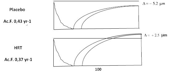
Figure 1: Reconstructed bone remodeling sequences in early postmenopausal women treated with MHT or placebo for 2 years. Bone resorption is shown on the left and the bone formation sequence on the right. One remodeling cycle lasts around 200 days. Note the development of a negative balance between resorption and formation in untreated women and the preservation of bone balance in women on MHT. Also note the reduction of the activation frequency (Ac.F), which is a histomorphometric measure of bone turnover. From Eriksen et al. J Bone Miner Res, 14(7), 1217-1221, with permission.

Clinical Effects of SERMS on Bone

SERMS (raloxifene, arzoxifene, lasofoxifene, basedoxifene) achieve less reduction of bone turnover hovering around 15-50% and in line with this lesser effect on bone turnover, BMD increases are also lower than those reported for HRT around 1-2,9% after 2-3 years [24-27]. All 4 SERMS reduce vertebral fractures by 30% (raloxifene 60 mg), 41% (arzoxifene 20 mg), 42% (lasofoxifene 0,5 mg) and 42% (basedoxifene 20 mg). The effects on nonvertebral fractures were only significant for lasofoxifene 0,5 mg (RRR 24%; p=0,02), but not significant for any of the other 3 SERMS and lasofoxifene 0,25 mg: basedoxifene reported significant reduction (50%) of nonvertebral fractures was demonstrable in a post hoc high-risk group (p=0,02) (Figure 2).

fig 2

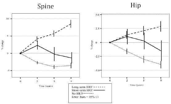
Figure 2: BMD over time in women treated with MHT for 2 years (short term HRT) and 9 years (long term HRT), compared to untreated women (No HRT). From Middleton ET & Steel SA Climacteric 2007; 10:257–263 with permission.

Safety

MHT

The initial conclusions from the WHI study emphasized an unfavorable risk/benefit ratio, mainly focusing on an increased risk of breast cancer, stroke and thromboembolism. The reduced risk of colon cancer, diabetes and reduced cancer and all-cause mortality also emerging from WHI [1], were rarely mentioned.

Later studies showed that the increased risk of breast cancer was mainly attributable to the progestogen component administered with estrogen to women with an intact uterus, as hysterectomized women given estrogen only did not display increased risk [28,29]. Moreover, the statistical analysis of the breast cancer risk in WHI has been called into question [28]. Finally, the discrepancy between WHI data and e.g. the DOPS data with respect to breast cancer risk may be partly due to estrogens used (13 different estrogen compounds in CEE used in WHI vs. 17b-estradiol used in DOPS) as well as a much different age profile.

The increased CV risk also depends on the woman´s age at initiation of therapy, with women below the age of 60 when starting MHT actually exhibiting protection against CV events, the so called “timing hypothesis” [29-31]. This notion is supported by a recent Cochrane analysis. It found that those who started hormone therapy less than 10 years after menopause exhibited 30% lower mortality and 48% reduction of coronary heart disease. The risk of venous thromboembolism was still increased by a factor 1,7 in estrogen treated subjects, but no detectable increase in stroke risk was demonstrable. Also worth noting, was the finding, that MHT initiation more than 10 years after menopause had little effect on risk of death or coronary heart disease, while risk of stroke and DVT were still increased by a factor 1,2 and 2,0 respectively. The findings of this Cochrane analysis are also of interest in light of the results obtained in the Danish DOPS study. In this study 1000 women, all below the age of 60, were randomized to either placebo of oral MHT. After 10 years, the study was stopped due to the findings of the WHI study, but women staying on HRT and placebo were still followed via health registers. After 10 years women on HRT showed a 52% lower risk of CV disease and CV death, and this risk reduction was preserved over 18 years in women staying on MHT. Breast cancer risk in hormone users was not increased in this study. Risk of thromboembolism was not increased significantly. The reanalysis of the mortality date emerging from WHI by Manson et al. [29] revealed that the Hazard ratio for all-cause mortality was 0.61 (95% CI, 0.43-0.87) during the intervention phase in WHI and 0.87 (95% CI, 0.76-1.00) during the cumulative 18-year follow-up after the trial.

Transdermal administration of estradiol has not been associated with increased risk of thromboembolism [32,33]. Micronized progesterone seems to reduce the risk of DVT, and has not been associated with increased breast cancer risk [33]. Medroxyprogesterone Acetate (MPA) has been associated with increased risk of both breast cancer and venous thrombosis.

Serms

Except for lasofoxifene, all SERMS have been associated with increased risk (RR 1,4-2,7) of venous thromboembolism [9,34-36]. This has to be weighed against significant reductions in risk of breast cancer (RR 0,19-0,44) demonstrated for raloxifene, arzoxifene and lasofoxifene [9,34-36]. Raloxifene increased risk of fatal stroke by 44% [37], but this has not been with other SERMS. Lasofoxifene has the ideal profile of a SERM. At a dose of 0.5 mg per day it reduced risks of nonvertebral and vertebral fractures, ER-positive breast cancer, coronary heart disease, but further development was stopped due to increased mortality in subjects treated with the lower dose of 0,25 mg [34].

Conclusions

The WHI data still form the basis for most safety considerations pertaining to MHT, and if you are a evidence based medicine purist, this will remain the case, until another well conducted similar sized randomized trial is published. However, with the price tag linked to such trials, this will probably not happen in the near future. We are therefore left with the sub-analyses emerging from WHI and other randomized trials like the Danish DOPS study, showing a much different safety profile. The interpretation depends on the relative weight one places on the different adverse effects, but to use WHI as the only basis for guidelines can certainly be discussed as emphasized by Langer et al. [28]. To me the long-term CV protection is crucial and outweighs other potential safety issues. Moreover, the thromboembolic risk seen with oral hormone administration seems to be absent with transdermal administration. The learning’s from the trials available can therefore in my view be summarized as follows:

  • MHT should be started in early menopause and not after the age of 60.
  • MHT should preferably be given by the transdermal route, as it reduces risk of venous thromboembolism.
  • Micronized progesterone is preferable to progestogen, but if the latter is used systemic exposure should be minimized (e.g. administration via intrauterine device).
  • If started before the age of 60, MHT reduces CV risk by 50%, and it can be continued beyond the age of 60 with continued CV protection.
  • MHT is also associated with reduced risk of diabetes and colon cancer.
  • The data on breast cancer risk associated with MHT are equivocal, and seem to depend on estrogen and progestogen used.
  • MHT before initiated before the age of 60 is associated with reduced all-cause mortality.
  • It should not be forgotten, that MHT will also improve general quality of life for most women by reducing hot flushes, improving sleep and sex life by improving libido and vaginal dryness.
  • MHT remains contraindicated in women with active or previous breast cancer. Also, women with hormone sensitive migraine also may encounter worsening of headaches.

In my view MHT therefore constitutes an effective and safe anti-osteoporotic medication for younger women with low bone mass at menopause with additional positive effects on health:

  • MHT reduces risks of both vertebral and non-vertebral fractures.
  • MHT is associated with a long-term continuous increase in bone mass, resulting in values in the upper normal range of normal after 10-15 years in most long-term users.
  • Even short-term use of MHT prevents accelerated bone loss in early menopause, and improves bone status in the long run, despite postmenopausal bone loss rates ensuing after discontinuation.
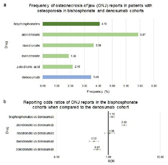
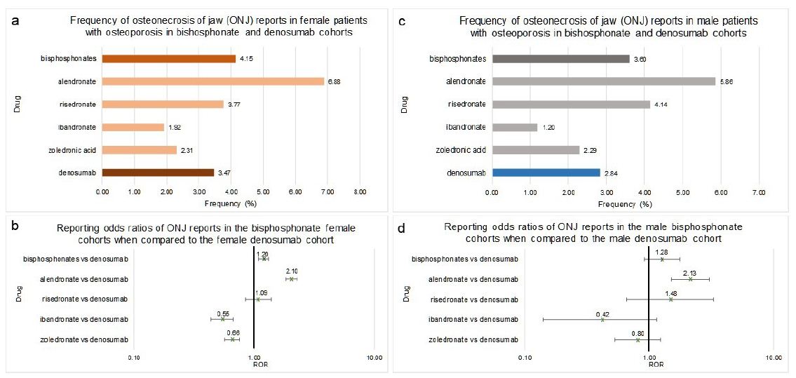
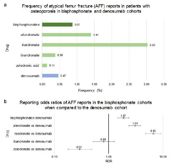
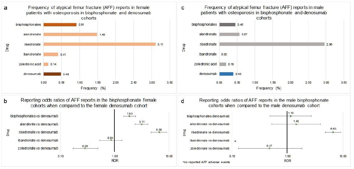
  • MHT has not been associated with very rare side effects like osteonecrosis of the jaw and atypical femoral fractures seen in long term users of bisphosphonates and denosumab.
  • In women with prevalent fractures, I would still prefer bisphosphonates possibly in combination with MHT, and in more severe cases osteoanabolic therapies like teriparatide or romosozumab.

The role of SERMS in the treatment of osteoporosis is in my view limited, due to the absence efficacy against non-vertebral fractures, which constitutes 75% of all clinical fracrtures. They remain, however, an option for women at high risk of breast cancer.

References

  1. Rossouw JE, Anderson GL, Prentice RL, LaCroix AZ, Kooperberg C, et al. (2002) Risks and benefits of estrogen plus progestin in healthy postmenopausal women: principal results From the Women’s Health Initiative randomized controlled trial. JAMA 288: 321-333. [crossref]
  2. Mirkin S, Komm B, Pickar JH (2014) Conjugated estrogen/bazedoxifene tablets for the treatment of moderate-to-severe vasomotor symptoms associated with menopause. Womens Health (Lond) 10: 135-146. [crossref]
  3. Cummings SR, Ettinger B, Delmas PD, Kenemans P, Stathopoulos V, et al. (2008) The effects of tibolone in older postmenopausal women. N Engl J Med 359: 697-708. [crossref]
  4. Eriksen EF, Colvard DS, Berg NJ, Graham ML, Mann KG, et al. (1988) Evidence of estrogen receptors in normal human osteoblast-like cells. Science 241: 84-86. [crossref]
  5. Oursler MJ, Landers JP, Riggs BL, Spelsberg TC (1993) Oestrogen effects on osteoblasts and osteoclasts. Ann Med 25: 361-371. [crossref]
  6. Khosla S, Oursler MJ, Monroe DG (2012) Estrogen and the skeleton. Trends Endocrinol Metab 23: 576-581. [crossref]
  7. Eriksen EF, Langdahl B, Vesterby A, Rungby J, Kassem M (1999) Hormone replacement therapy prevents osteoclastic hyperactivity: A histomorphometric study in early postmenopausal women. J Bone Miner Res 14: 1217-1221. [crossref]
  8. Khastgir G, Studd J, Holland N, Alaghband-Zadeh J, Fox S, et al. (2001) Anabolic effect of estrogen replacement on bone in postmenopausal women with osteoporosis: histomorphometric evidence in a longitudinal study. J Clin Endocrinol Metab 86: 289-295. [crossref]
  9. Ettinger B, Black DM, Mitlak BH, Knickerbocker RK, Nickelsen T, et al. (1999) Reduction of vertebral fracture risk in postmenopausal women with osteoporosis treated with raloxifene: results from a 3-year randomized clinical trial. Multiple Outcomes of Raloxifene Evaluation (MORE) Investigators. JAMA 282: 637-645. [crossref]
  10. Paech K, Webb P, Kuiper GG, Nilsson S, Gustafsson J, et al. (1997) Differential ligand activation of estrogen receptors ERalpha and ERbeta at AP1 sites. Science 277: 1508-1510. [crossref]
  11. Weinstein RS, Parfitt AM, Marcus R, Greenwald M, Crans G, et al. (2003) Effects of raloxifene, hormone replacement therapy, and placebo on bone turnover in postmenopausal women. Osteoporos Int 14: 814-822. [crossref]
  12. Bauer DC, Black DM, Garnero P, Hochberg M, Ott S, et al. (2004) Change in bone turnover and hip, non-spine, and vertebral fracture in alendronate-treated women: the fracture intervention trial. J Bone Miner Res 19: 1250-1258. [crossref]
  13. Rogers A, Glover SJ, Eastell R (2009) A randomised, double-blinded, placebo-controlled, trial to determine the individual response in bone turnover markers to lasofoxifene therapy. Bone 45: 1044-1052. [crossref]
  14. Lindsay R, Hart DM, Aitken JM, MacDonald EB, Anderson JB, et al. (1976) Long-term prevention of postmenopausal osteoporosis by oestrogen. Evidence for an increased bone mass after delayed onset of oestrogen treatment. Lancet 1: 1038-1041. [crossref]
  15. Christiansen C, Christensen MS, McNair P, Hagen C, Stocklund KE, et al. (1980) Prevention of early postmenopausal bone loss: controlled 2-year study in 315 normal females. Eur J Clin Invest 10: 273-279. [crossref]
  16. Evio S, Tiitinen A, Laitinen K, Ylikorkala O, Valimaki MJ (2004) Effects of alendronate and hormone replacement therapy, alone and in combination, on bone mass and markers of bone turnover in elderly women with osteoporosis. J Clin Endocrinol Metab 89: 626-631. [crossref]
  17. Middleton ET, Steel SA (2007) The effects of short-term hormone replacement therapy on long-term bone mineral density. Climacteric 10: 257-263. [crossref]
  18. Naessen T, Persson I, Thor L, Mallmin H, Ljunghall S, et al. (1993) Maintained bone density at advanced ages after long term treatment with low dose oestradiol implants. Br J Obstet Gynaecol 100: 454-459. [crossref]
  19. Heikkinen J, Vaheri R, Kainulainen P, Timonen U (2000) Long-term continuous combined hormone replacement therapy in the prevention of postmenopausal bone loss: a comparison of high- and low-dose estrogen-progestin regimens. Osteoporos Int 11: 929-937. [crossref]
  20. Black DM, Delmas PD, Eastell R, Reid IR, Boonen S, et al. (2007) Once-yearly zoledronic acid for treatment of postmenopausal osteoporosis. N Engl J Med 356: 1809-1822. [crossref]
  21. Cummings SR, San MJ, McClung MR, Siris ES, Eastell R, et al. (2009) Denosumab for prevention of fractures in postmenopausal women with osteoporosis. N Engl J Med 361: 756-765. [crossref]
  22. Bagger YZ, Tanko LB, Alexandersen P, Hansen HB, Mollgaard A, et al. (2004) Two to three years of hormone replacement treatment in healthy women have long-term preventive effects on bone mass and osteoporotic fractures: the PERF study. Bone 34: 728-735. [crossref]
  23. Watts NB, Cauley JA, Jackson RD, LaCroix AZ, Lewis CE, et al. (2017) No Increase in Fractures After Stopping Hormone Therapy: Results From the Women’s Health Initiative. J Clin Endocrinol Metab 102: 302-308. [crossref]
  24. Delmas PD, Bjarnason NH, Mitlak BH, Ravoux AC, Shah AS, et al. (1997) Effects of raloxifene on bone mineral density, serum cholesterol concentrations, and uterine endometrium in postmenopausal women. N Engl J Med 337: 1641-1647. [crossref]
  25. Johnston CC, Bjarnason NH, Cohen FJ, Shah A, Lindsay R, et al. (2000) Long-term effects of raloxifene on bone mineral density, bone turnover, and serum lipid levels in early postmenopausal women: three-year data from 2 double-blind, randomized, placebo-controlled trials. Arch Intern Med 160: 3444-3450. [crossref]
  26. Lufkin EG, Whitaker MD, Nickelsen T, Argueta R, Caplan RH, et al. (1998) Treatment of established postmenopausal osteoporosis with raloxifene: a randomized trial. J Bone Miner Res 13: 1747-1754. [crossref]
  27. Silverman SL, Christiansen C, Genant HK, Vukicevic S, Zanchetta JR, et al. (2008) Efficacy of bazedoxifene in reducing new vertebral fracture risk in postmenopausal women with osteoporosis: results from a 3-year, randomized, placebo-, and active-controlled clinical trial. J Bone Miner Res 23: 1923-1934. [crossref]
  28. Langer RD, Simon JA, Pines A, Lobo RA, Hodis HN, et al. (2017) Menopausal hormone therapy for primary prevention: why the USPSTF is wrong. Climacteric 20: 402-413. [crossref]
  29. Manson JE, Aragaki AK, Rossouw JE, Anderson GL, Prentice RL, et al. (2017) Menopausal Hormone Therapy and Long-term All-Cause and Cause-Specific Mortality: The Women’s Health Initiative Randomized Trials. JAMA 318: 927-938. [crossref]
  30. Manson JE, Allison MA, Rossouw JE, Carr JJ, Langer RD, et al. (2007) Estrogen therapy and coronary-artery calcification. N Engl J Med 356: 2591-2602. [crossref]
  31. Schierbeck LL, Rejnmark L, Tofteng CL, Stilgren L, Eiken P, et al. (2012) Effect of hormone replacement therapy on cardiovascular events in recently postmenopausal women: randomised trial. BMJ 345: e6409.
  32. Olie V, Canonico M, Scarabin PY (2011) Postmenopausal hormone therapy and venous thromboembolism. Thromb Res 127: S26-29. [crossref]
  33. Tremollieres F, Brincat M, Erel CT, Gambacciani M, Lambrinoudaki I, et al. (2011) EMAS position statement: Managing menopausal women with a personal or family history of VTE. Maturitas 69: 195-198. [crossref]
  34. Cummings SR, Ensrud K, Delmas PD, LaCroix AZ, Vukicevic S, et al. (2010) Lasofoxifene in postmenopausal women with osteoporosis. N Engl J Med 362: 686-696. [crossref]
  35. Cummings SR, McClung M, Reginster JY, Cox D, Mitlak B, et al. (2010) Arzoxifene for prevention of fractures and invasive breast cancer in postmenopausal women. J.Bone Miner.
  36. Siris ES, Harris ST, Eastell R, Zanchetta JR, Goemaere S, et al. (2005) Skeletal effects of raloxifene after 8 years: results from the continuing outcomes relevant to Evista (CORE) study. J Bone Miner Res 20: 1514-1524. [crossref]
  37. Barrett-Connor E, Mosca L, Collins P, Geiger MJ, Grady D, et al. (2006) Raloxifene Use for The Heart Trial, I. Effects of raloxifene on cardiovascular events and breast cancer in postmenopausal women. N Engl J Med 355: 125-137. [crossref]

Clomiphene Citrate is a Safe and Effective Alternative to Testosterone Replacement in Male Hypogonadism with Type 2 Diabetes Mellitus

DOI: 10.31038/EDMJ.2021512

Abstract

Aims: The study was planned to evaluate the effect of Clomiphene Citrate (CC) treatment as compared to testosterone replacement for late onset hypogoandism in  with type 2 Diabetes Mellitu.

Methods: The study included 72 male patients with late onset hypogonadism (assessed by ADAM questionnaire, serum total testosterone and LH) and T2DM out of 250 patients screened. The subjects with serum testosterone in the range of 200-300 ng/dl and with serum Luteinizing hormone (LH) level ≤9.4 IU/ml were treated with Clomiphene Citrate 25 mg/day (Group 1 N= 40). Patients with serum testosterone levels less than 200 ng/dl and serum LH < 9.4 IU/ml received testosterone every month for 3 months (Group 2 N=32). The post treatment hormone estimation along with ADAM questionnaire value was evaluated 3 month after commencing treatment.

Results: ADAM symptom scores were worse in group 2 (N=32) than group 1 (N= 40 ). There was a comparable increase in mean testosterone levels in both groups at 3 months (550.16 ± 85.05 vs 509.72 ± 39.18 ng/dl; p = 0.03). Mean ADAM scores also decreased significantly in both the groups.

Conclusion: Treatment with clomiphene citrate in male patients with T2DM and hypogonadism showed improvement in both clinical and biochemical measures. The study suggested that clomiphene citrate might be considered as a safe and effective alternative treatment strategy for late onset hypogonadism in male patients with type 2 DM.

Keywords

Hypogonadism, Clomiphene Citrate, Testosterone replacement, Type 2 diabetes mellitus

Introduction

Prevalence of type 2 diabetes mellitus (T2DM) is increasing worldwide to reach epidemic proportions [1]. Insulin resistance (IR) of variable degree is a feature of T2DM. It is recognized that low testosterone level in men is associated with reduced insulin sensitivity and T2DM. [2]. Epidemiological studies have reported that 30% – 50% of men with T2DM have testosterone deficiency, and up to 75% of them have sexual symptoms, particularly erectile dysfunction (ED)[3]. Dhindsa et al. demonstrated that 33% of men with type 2 diabetes had significantly lower levels of testosterone[4].

Questionnaires have been developed to assess hypogonadism. Androgen deficiency in the aging male (ADAM) questionnaire is one of them with a reasonable sensitivity (88%) and specificity (66%) in the presence of low testosterone levels.[5] In EMAS ( European Male Aging Study), subjects are classified into primary hypogonadism (LH > 9.4 u/L, T < 10.5 nmol/L), secondary hypogonadism (LH ≤ 9.4 u/L, T < 10.5 nmol/L) or compensated (primary) hypogonadism (LH > 9.4 u/L, T ≥ 10.5 nmol/L).[6]

Until very recently, treatment options mainly consisted of testosterone replacement using a variety of modalities but exogenous testosterone has unacceptable side effects. In many small studies clomiphene citrate (CC) has shown promising efficacy. As a selective estrogen receptor modulator (SERM), it acts on the Hypothalamic – Pituitary – Gonadal (HPG) axis and increases gonadotrophin levels. In turn this also stimulates testosterone production and corrects androgen deficiency but its role improve hypogonadal symptoms in males with T2DM are lacking.[7] The present study was planned to evaluate the effect of treatment with clomiphene citrate as compared to testosterone replacement  for hypogonadism in patients with T2DM, based on both symptoms and biochemical measures.

Subjects

This study was conducted in the Department of Endocrinology and Metabolism, Sir Sunderlal Hospital, Institute of Medical Sciences, BHU, Varanasi. Study subjects were enrolled from April 2016 to June 2017. Subjects with T2DM with biochemical (Testosterone < 300 ng/dl with low LH <9.4 IU/ml ) and symptomatic hypogonadism, aged 40–70 years with no serious concurrent medical conditions were enrolled. Patients were included in the study after obtaining their informed consent. The exclusion criteria were subjects on drug treatment which might cause HPG axis suppression, subjects with history of tumor, exposure to radiation, history of head trauma, spinal cord injuries, and history of pelvic trauma or with chronic disease such as human immunodeficiency virus, end-stage renal disease, liver cirrhosis, and psychiatric disease. A detailed clinical evaluation was done and recorded.

A total of 250 patients underwent screening for symptoms of hypogonadism by ADAM questionnaire. This is a 10 question validated questionnaire focusing on key clinical feature of hypogonadism (Appendix).

Material & Methods

All cases who had positive response based on decrease in loss of libido, strength of erections or any three nonspecific questions that included fatigability, mood changes and loss of height were subjected to biochemical investigations like serum Testosterone (total) , LH , Prolactin, Thyroid function test, Hemogram, fasting Lipid profile, HbA1c, Serum Creatinine and serum prostate specific antigen(PSA).

Patients with serum LH level in the low or normal range (≤9.4 IU/ml) and Testosterone < 300 ng/dl (Lower than Normal reference range 300-1000 ng/dl of our laboratory) were informed of their candidacy for treatment. The subjects were divided into two groups, Group I with serum Testosterone < 200ng/dl were given Testosterone intramuscular injection monthly for 3 months and Group II with S. testosterone between 200- 300 ng/dl were given Clomiphene citrate (CC) 25mg daily PO for 3 months. All patients received counseling on diet and exercise consistent with American Diabetes Association recommendations throughout the study. Each of the participants was given verbal information and were asked to report if they experienced any side effect related to the use of treatment. The post treatment hormone estimation along with ADAM questionnaire value was conducted 3 months after commencing treatment. The study was approved by the local Ethics committee.

Special Investigations – Total testosterone (twice) and LH was measured by chemiluminescence immunoassay (Beckman Coulter, USA). In patient with diabetes, blood sample was collected always between 8 a.m. and 10 am in the fasting state. Serum was obtained by centrifugation and stored at –20°C for assay in a batch.

Statistics -Data were collected, revised, coded, and entered in the statistical package for social science (IBM SPSS) version 16. The qualitative data were presented as numbers and percentages while the quantitative data were presented as means, standard deviations. The comparison between two groups with qualitative data was done by using Chi-square test while the comparison between two groups with quantitative data and parametric distribution were done by using independent t-test. Spearman correlation coefficients were used to assess the significance between two quantitative parameters in the same group. The confidence interval was set to 95% and the margin of error accepted was set to 5%. P-value was considered significant at the level of <0.05.

Results

The baselisne characteristics of the study population are shown in Table 1.  Both the groups were comparable. All subjects were between 40 to 70 years of age and mean age was 49.52 ± 6.64 years (SD). Duration of diabetes was more in group 2 in comparison to group 1 (7.76 ± 2.97 vs 6.36 ± 3.28, p = 0.12). Both the groups were comparable at baseline for PSA, LH and HbA1c (p value >0.05) while the mean testosterone level for group 1 was 279.68 ± 20.23 (range 257.45-299.91 ng/dl) and for group 2 was 158.69 ± 39.04 (range 62.87-199.7), p value <0.001. Mean ADAM score was significantly higher in group 2 in comparison to group 1 (8.36 ± 0.64 vs 7.52 ± 1.36). {Table 2}.

Table 1: Baseline Characteristics of Study Population

Characteristics

Group 1 (CC)

N =40

Group 2 (TT)

N=32

p-value

Age

47.92 ± 6.64

51.12 ± 6.37

0.088

Height (cm)

165.38 ± 5.65

165.34 ± 5.36

0.980

Weight (kg)

71.52 ± 10.90

71.68 ± 7.98

0.952

BMI (kg/m2)

26.16 ± 3.14

26.25 ± 2.35

0.905

Waist circumference (cm)

94.06 ± 8.09

92.96 ± 6.07

0.589

Hip circumference (cm)

95.41 ± 4.92

93.77 ± 3.81

0.192

Waist Hip Ratio

0.97 ± 0.05

0.99 ± 0.05

0.632

Diabetes duration (years)

6.36 ± 2.97

7.76 ± 3.28

0.120

Hemoglobin (gm%)

13.72 ± 0.82

13.08 ± 0.80

0.009

Prolactin (ng/ml)

7.22 ± 3.22

7.16 ± 2.40

0.939

TSH (mU/l)

2.66 ± 1.32

2.68 ± 1.05

0.979

Hematocrit (%)

43.22 ± 1.85

42.26 ± 1.39

0.042

S.Creatinine (mg/dl)

0.98 ± 0.19

1.00 ± 0.13

0.750

PSA

0.95± 0.58

0.79 ± 0.30

0.233

HbA1c

8.91 ± 1.29

9.31 ± 1.68

0.354

ADAM

7.52± 1.36

8.36± 0.64

0.007

Testosterone

279.68 ± 20.23

158.69 ± 39.04

0.000

LH

4.49 ± 1.17

4.53 ± 0.88

0.912

After treatment for 3 months with Clomiphene Citrate and testosterone in group 1 and 2 respectively there was significant reduction in ADAM score in comparison to baseline. (7.52 ± 1.36 at baseline to 2.68 ± 0.90 after 3 months in group 1, p<0.001;8.36± 0.64 at baseline to 3.24± 0.83 after 3 months in group 2,p<0.001). Similarly there was a significant improvement in mean testosterone levels in both the groups after 3 months of treatment (279.68 ± 20.23 ng/dl to 550.16 ± 85.05 in group 1 , p<0.001 ; 158.68 ± 39.04 to 509.72 ± 39.18 in group 2 , p< 0.001). {Table 2}

Table 2: Analysis of group 1 (Clomiphene Citrate) group II (testosterone treated) patients before and after treatment:


Group I  (CC)
N=40

Group II (TT)
N=32

parameters

Pre
Mean ± SD

Post
Mean ± SD
p-value Pre
Mean ± SD
Post
Mean ± SD

p-value

Hematocrit

43.22 ±1.85

43.99 ± 1.95 0.016 42.26 ± 1.39 43.26 ± 0.93

<0.001

PSA

0.95 ± 0.58

0.99 ± 0.52 0.153 0.79 ± 0.29 0.856± 0.28

0.044

Creatinine

0.98 ± 0.19

0.99 ± 0.16 0.799 1.00 ± 0.13 0.99 ± 0.13

0.829

HbA1c

8.92 ± 1.29

8.14 ± 0.98 <0.001 9.31 ± 1.67 8.83 ± 1.23

0.001

LH

4.49±1.17

7.49 ± 1.60 <0.001 4.52 ± 0.87 4.03 ± 0.74

<0.001

ADAM score

7.52± 1.36

2.68 ± 0.90  <0.001 8.36± 0.64 3.24± 0.83

<0.001

Total testosterone

279.68 ± 20.23

550.16 ± 85.05 <0.001 158.68 ± 39.04 509.72 ± 39.18

<0.001

Discussion

The type 2 DM has been recognized as a risk factor for male hypogonadism by most of the international endocrinology and andrology societies in their recommendations. [8] The hypogonadism in diabetic male has been defined on the basis of serum total testosterone in most of the studies but clinical symptoms of hypogonadism have been rarely considered in combination with testosterone deficiency. [9] In the present study, we used combination of both clinical (ADAM) and biochemical androgen deficiency to define hypogonadism.

Epidemiological[8]  studies have reported testosterone deficiency in 30%– 50% of men with T2DM and up to 75% of them having sexual dysfunction. In our study, it was found that 118 (47.2%) men had symptoms of androgen deficiency, while 72 (28.8%) men had both symptoms and biochemical testosterone deficiency.

Our study showed that treatment of hypogonadism with Clomiphene citrate in comparison to testosterone therapy had similar degree of improvement in both clinical (ADAM) and biochemical (total testosterone) parameters. Clomiphene Citrate has been evaluated in hypogonadal patients [10] but this is the first study to compare Clomiphene with testosterone in male T2DM patients with hypogonadism.

Therapy in both the groups was shown to improve glycemic control. This observation is in line with previous studies. [11] Not surprisingly, treatment of hypogonadism has a significant positive impact on the health related quality of life in affected men. None of our study subjects in both the groups had reported any major side effect which required change/discontinuation of treatment.

The strength of our study was  a prospective design assessing both the clinical response based on ADAM questionnaire as well as the biochemical response based on serum total testosterone levels. The weaknesses of our study included reasonable but small number of patients,  short term follow up, lack of estimation of free testosterone and SHBG levels and limitations associated with ADAM questionnaire.

Conclusions

Treatment of secondary hypogonadism with Clomiphene Citrate in male patients with T2DM showed improvement in both clinical and biochemical measures of a similar degree and a tolerability profile that did not differ from that of testosterone therapy. It might be considered as an effective and safe alternative treatment strategy in secondary hypogonadal diabetic patients. Further long-term studies in a large cohort of patients with T2DM and hypogonadism are needed to evaluate  the impact on metabolic parameters.


APPENDIX 1: ADAM QUESTIONNAIRE:

  1. Do you have a decrease in libido (sex drive)?
  2. Do you have a lack of energy?
  3. Do you have a decrease in strength and/or endurance?
  4. Have you lost height?
  5. Have you noticed a decreased “enjoyment of life”?
  6. Are you sad and/or grumpy?
  7. Are your erections less strong?
  8. Have you noted a recent deterioration in your ability to play sports?
  9. Are you falling asleep after dinner?
  10. Has there been a recent deterioration in your work performance?

This questionnaire is suggestive of the presence of HG when the patient answers ‘yes’ to items 1 or 7 or when 3 or more questions are answered affirmatively.

References

  1. Gupta R, Misra A. (2007) Review: Type 2 diabetes in India: regional disparities. The British Journal of Diabetes &amp; Vascular Disease 7(1):12–6.
  2. Reaven GM. Banting lecture 1988. Role of insulin resistance in human disease. Diabetes 37(12):1595–607.[cross-ref]
  3. Mulligan T, Frick MF, Zuraw QC, Stemhagen A, Mcwhirter C. et al.( 2008) Prevalence of hypogonadism in males aged at least 45 years: the HIM study. International Journal of Clinical Practice 60(7):762–9.[cross-ref]
  4. Dhindsa S, Prabhakar S, Sethi M, Bandyopadhyay A, Chaudhuri A, Dandona P. et al.(2004) Frequent Occurrence of Hypogonadotropic Hypogonadism in Type 2 Diabetes. The Journal of Clinical Endocrinology & Metabolism 89(11):5462-5468. [cross-ref]
  5. Morley JE, Perry III HM, Kevorkian RT, Patrick P. et al.(2006) Comparison of screening questionnaires for the diagnosis of hypogonadism. Maturitas 53:424–9. [cross-ref]
  6. Tajar A, Forti G, O’Neill T, Lee D, Silman A, Finn J et al.(2010) Characteristics of Secondary, Primary, and Compensated Hypogonadism in Aging Men: Evidence from the European Male Ageing Study. The Journal of Clinical Endocrinology & Metabolism 95(4):1810-1818.[cross-ref]
  7. Moskovic D, Katz D, Akhavan A, Park K, Mulhall J. et al.(2012) Clomiphene citrate is safe and effective for long-term management of hypogonadism. BJU International 110(10):1524-1528.[cross-ref]
  8. Corona G, Monami M, Rastrelli G, Aversa A, Sforza A, Lenzi A et al.(2010) Type 2 diabetes mellitus and testosterone: a meta-analysis study. International Journal of Andrology 34(6pt1):528-540.[cross-ref]
  9. Kapoor D, Aldred H, Clark S, Channer KS, Jones TH. et al.(2007) Clinical and biochemical assessment of hypogonadism in men with type 2 diabetes: correlations with bioavailable testosterone and visceral adiposity. Diabetes Care 30:911–917.[cross-ref]
  10. Guay A, Jacobson J, Perez J, Hodge M, Velasquez E. et al.(2003) Clomiphene increases free testosterone levels in men with both secondary hypogonadism and erectile dysfunction: who does and does not benefit?. International Journal of Impotence Research 15(3):156-165.[cross-ref]
  11. Katz D, Nabulsi O, Tal R, Mulhall J. et al.(2011) Outcomes of clomiphene citrate treatment in young hypogonadal men. BJU International 110(4):573-578.

Identification of Phosphoglucomutase as an Enteropathogen Growth Stimulating Factor

DOI: 10.31038/NRFSJ.2021413

Abstract

A highly selective Salmonella and Shiga Toxin-producing E. coli (STEC) enrichment medium broth (SSS; commercially known as PDX-STEC), in comparative studies of low level E. coli O157:H7 inoculated ground beef and spinach, showed a 50- to 100- fold increase in STEC recoveries of the pathogen from ground beef compared to spinach enrichments. These observations suggested that either a soluble component of spinach inhibited the growth of the E. coli O157:H7 or a soluble component of ground beef stimulated the growth of the pathogen. The growth stimulating effect was linked to a soluble component of ground beef by comparing the growth of STEC and Salmonella in SSS conditioned with ground beef by passive extraction to their growth in control SSS containing traditional powdered beef extract media supplement. Then attempts were made to isolate and identify the responsible compound(s). A 20 to 60% ammonium sulfate fraction of ground beef extract maintained the growth stimulation of STEC and Salmonella. Further purification using affinity chromatography and preparative polyacrylamide gel electrophoresis identified three specific protein bands (52 kD, 35 kD and 20 kD) associated with the growth stimulating activity. Mass spectral analysis of the trypsin-digested peptides of these proteins provided a putative identification of the proteins as the glycolytic protein, phosphoglucomutase (E.C.5.4.2.2). Finally, commercially prepared rabbit muscle Phosphoglucomutase (PGM) was shown to have the same growth stimulating activity thereby confirming the identity of the active protein. The possible mechanisms of growth stimulation by PGM may be through increasing bacterial fitness and environmental adaptability. Inclusion of PGM in food safety test protocols can enhance detection and isolation of contaminating STEC and Salmonella.

Highlights/Significance

  • A putative growth stimulating factor was linked to 20 kD, 35 kD and 52 kD proteins.
  • Mass spectral analysis provided a provisional identification of the protein as Phosphoglucomutase (PGM) which was then confirmed using a commercially available PGM.
  • This protein can be used as an enrichment media supplement to improve the detection and recovery of STEC and Salmonella in foods.

Keywords

Food safety, Shiga toxin-producing E. coli, Salmonella, Selective enrichment

Introduction

Food borne illness linked to Shiga Toxin-producing Escherichia coli (STEc) and Salmonella enterica is on-going problem in the United States. United States Department of Agriculture (USDA) Food Safety and Inspection Service (FSIS) recalls involving these pathogens were reported in 2019 and 2020 in various food stuffs [1-3]. The US Food and Drug Administration (FDA) initiated recalls during the same period involved cantaloupe [4], cinnamon apple chips [5], peaches [6] and flour [7]. The frequency and breadth of food stuffs contaminated with STEC and Salmonella demonstrate that there are challenges in the available testing methodologies to properly assess the food safety systems producing these food products. The challenges in food testing methodologies may permit contaminated food to enter the national food supply.

E coli is usually a harmless bacterium living in the gastrointestinal tract of humans and other mammals. There are different serotypes of E. coli that have acquired bacterial Shiga toxin genes, originally arising in Shigella. The most prominent STEC associated with severe human disease in the US is E. coli O157:H7. This serotype is associated with cattle, its natural reservoir and can contaminate beef products during harvest and processing. Six other serogroups of STEC (O26, O45, O103, O111, O121 and O145) are responsible for about three-quarters of non-O157 STEC illness in the US [8]. These multiple serotypes and serogroups of pathogenic E. coli can be indistinguishable from the harmless E. coli of the gastrointestinal tract and thus pose a challenge for detection and isolation. Likewise, the CDC has identified Salmonella serotypes Enteritids, Newport, Typhimurium, and Javiana as the most common serotypes causing reportable Salmonellosis [9]. Although these are the most frequently reported Salmonella serotypes overall, their attribution to various food stuffs varies [10], with serotypes Typhimurium and Newport most commonly attributed to beef, while Enteritidis is attributed to chicken and eggs, and less common serotypes like Heidelberg attributed to turkey products. Even uncommon Salmonella serotypes such as Tennessee have been observed to emerge as significant outbreak strains, as occurred in 2006 associated with peanut butter [9].

The technical challenges of distinguishing these gram-negative pathogens from harmless gastrointestinal coliforms has been rendered substantially less difficult with the advent of PCR screening methods that target specific portions of the E. coli O157:H7 genome or common virulence factors such as the Shiga toxin gene (stx) present in STEC [11]. Similar molecular methods targeting virulence markers such as the invasion gene (invA) of Salmonella allow detection of most Salmonella serotypes [12]. Regardless of the detection method used, food samples contaminated by STEC and Salmonella must be enriched in a broth medium that increases the concentration of the pathogen to a detectable level, which is approximately 4 to 5 log10 CFU/mL for most methods. Reaching this effective level can be challenging due to the outgrowth of other naturally present contaminating flora [13]. Numerous methods are used to enhance target pathogen growth such as incubation at restrictive temperatures (eg: 42°C) or inclusion of various antimicrobial compounds [14-16].

In a previous publication we detailed the development of a highly selective enrichment medium for detection and isolation of STEC and Salmonella from ground beef [14]. The media was shown to substantially reduce the complexity of the methods described in the USDA FSIS Microbiological Laboratory Guidebook (MLG) [15]. This was achieved by utilization of selective antimicrobials and inclusion of an efflux pump inhibitor that reduced the growth of background microbiological flora in the food matrix. While the medium was selective, during further validation experiments it was observed to be only effective in beef products rather than all food matrices tested. It was hypothesized that a component inherent in meat was enhancing the growth of STEC and Salmonella. In this report we describe the studies that isolated and characterized the molecular nature of the growth stimulating factor present in ground beef.

Materials and Methods

Approach

The testing of our hypothesis was addressed through the following four experiments:

Experiment 1

Media conditioned with ground beef extract was compared to media containing traditional powdered beef extract supplement as control to verify STEC and Salmonella growth stimulation was directly related to the presence of fresh ground beef.

Experiment 2

Ammonium sulfate precipitation and fractionation, and molecular weight fractionation of ground beef extracts were performed to determine if a specific fraction contained the growth stimulating activity.

Experiment 3

Identification of compound(s) in the active ammonium sulphate fraction was performed by affinity chromatography and preparative SDS-polyacrylamide gel electrophoresis followed by mass spectral analysis of suspect tryptic peptides.

Experiment 4

Commercial sourced biomolecules were obtained and tested for growth stimulating activity to confirm the identity of the active compound(s) Figure 1.

FIG 1

Figure 1: Flow chart of experimental approach.

Media and Media Ingredients

Tryptic Soy Broth (TSB), MI (MUG: methylumbelliferyl-beta-D-galactopyranoside; IBDG: Inoxyl-beta-D-glucuronide) Agar, Brain Heart Infusion (BHI), Buffered Peptone Water, were obtained from Becton Dickinson (Franklin Lakes, NJ). Tryptic Soy Agar (TSA), D-Raffinose, D-Arabinose, Bromocresol Purple, Peptone from casein, D-Xylose were obtained from Sigma-Aldrich (St. Louis, MO). D-Sorbitol was obtained from Fisher Scientific (Hampton, NH). Trehalose was obtained from GoldBio (St. Louis, MO). Bile salt was obtained from Honeywell Fluka (Charlotte, NC). CHROMagarTM STEC and CHROMagarTM SALMONELLA PLUS and were obtained from CHROMagar (Paris, France). The SSS medium, commercially known as PDX-STEC, was prepared according to instructions from the U.S. Patent: 9518283 [17], with the addition of 0.025% (m/v) bromocresol purple. The modified SSS medium or m-SSS medium was prepared by removing sulfanilamide and myricetin from the formulation. Modified tryptic soy broth (mTSB) was prepared by adding 0.15% (w/v) bile salts and 0.0008% (w/v) sodium novobiocin obtained from Sigma Aldrich, Milwaukee, WI. Modified buffered peptone water (mBPWp) was prepared according to the Bacteriological Analytical Manual of the US Food and Drug Administration [18]. Cibacron Blue 3GA was purchased from Polysciences (Warrington, PA).

Bacterial Strains

STEC and Salmonella strains were obtained from the Penn State University E. coli Reference Center in University Park, Pennsylvania, the Center for Disease Control and Prevention in Atlanta, Georgia, the U.S. Meat Animal Research Center (USDA Agricultural Research Services) in Clay Center, Nebraska, the American Type Culture Collection (ATCC) in Manassas, Virginia, and the University of Minnesota Veterinary Diagnostic Laboratory in Saint Paul, Minnesota. Bacterial cultures were maintained as glycerol stock at -20°C and revived in TSB incubated at 37°C overnight before use.

E. coli Growth Stimulating Activity Assays

In Experiments 1 and 2 the growth effects of medium with and without putative stimulating factors were assayed by inoculating 3.0 mL of modified SSS medium or mBPWp with a STEC or Salmonella strain at ~1 CFU/mL. After 7 h of incubation at 37°C, 0.1 mL aliquots of the samples were spread plated on CHROMAGAR™ STEC or CHROMAGAR SALMONELLA PLUS then incubated for 18 hours at 37°C. Bacterial populations were enumerated the following day by colony counts. In Experiments 3 and 4 growth stimulating assays used 1.0 mL portions of SSS medium prepared with purified components or commercial proteins, inoculated with 5-6 CFU/mL of E. coli O157:H7, that were then incubated at 37°C for six hours, after which 0.1 mL was plated onto Chromagar STEC medium. The plates were incubated at 37°C overnight and enumerated the following day.

Time-course experiments were conducted to monitor the growth stimulating activity on STEC and Salmonella in media with and without putative stimulating factors where 100-μL aliquots were withdrawn at 3, 5, and 7 hours and plated onto CHROMAGAR™ STEC or CHROMAGAR SALMONELLA PLUS, incubated and scored as described above.

Assessing Growth Stimulating Factor in Alternate Medium

Wheat kernels (25 g) were placed in stomacher bags then inoculated with ~3 CFU of E. coli O157:H7 and held at room temperature for 20 minutes. Two hundred milliliters of mBPWp, or mBPWp supplemented with 10% (v/v) of the F-1 ammonium sulfate cut (described below) was added to the stomacher bags. The samples were enriched at 42°C for seven hours, and 0.1-mL aliquots were taken at 2-hour intervals and spread onto CHROMAGAR™ STEC plates then incubated overnight at 37°C. Mauve colonies were enumerated.

Conditioning Media

The hypothesized stimulating factor was extracted into SSS medium by incubation of ground beef in ~3:1 v/m ratio where 165 g ground beef (80:20 lean:fat) was suspended in 500 mL SSS medium and stirred for thirty minutes at 10°C. The medium was decanted through a screen in a stomacher bag and filtered through a Celite pad to provide the conditioned medium. The conditioned medium was sterilized by filtration through a 0.22 mm filter.

Extraction Procedure

Ground beef (80:20 lean:fat) was obtained from a local grocery store. Ground beef extracted was prepared by suspending 4:1 v/m in 0.02 M Tris-Cl, pH 7.9, 0.032 M MgCl2, 0.027% w/v Niaproof-4. Extracts were clarified by filtration through course screen in stomacher bags followed by filtration through Celite 545 (Sigma-Aldrich, St. Louis, MO).

Ammonium Sulfate Precipitation and Fractionation

Initial ammonium sulfate fractionation was carried out at 100% saturation to determine if the active component was salt perceptible. To 100 mL extract of the ground beef (see above), 72.9 g of solid ammonium sulfate was added with stirring at 10°C. After 30 minutes, the sample was centrifuged in a MyFuge Mini Centrifuge™, Benchmark Scientific, Edison, NJ, at 6,000 RPM to pellet the precipitate. The supernatant was collected, and the pellet was re-dissolved in 3 mL of 0.01 M Tris-Cl pH 7.8. The resuspended pellet was dialyzed against same buffer to desalt. This initial total fraction was termed “F-1”.

Ammonium sulfate fractionation was carried out by addition of solid ammonium sulfate to obtain 20% and 60% saturation. The protein precipitates obtained at all ammonium sulfate saturation levels were collected by filtration through glass fiber filters and redissolved in a minimum volume of 0.02 M Tris-Cl, pH 7.9. The ammonium sulfate fraction obtained from 20% to 60% saturation was designated “AS-20/60”.

Ammonium sulfate precipitate F-1 and fraction AS-20/60 were prepared in SSS medium to a final concentration of 10% v/v for use in Experiment 2 growth studies with STEC and Salmonella cultures (see above).

Additional Purification Procedures

The F-1 precipitate was further purified using molecular weight cut off filters as follows: The F-1 preparation was ultrafiltered using an Amicon stirred ultrafiltration cell with a 50 and 100 -kD nominal Molecular Weight Cut-off (MWCO) membranes purchased from Sterlitech (Kent, WA). The retentate and filtrate fractions were prepared at 10 % v/v in SSS medium to assayed in Experiment 2 for E. coli growth stimulating activity (above).

The AS-20/60 fraction was further purified on a Cibacron Blue Sephadex column prepared according procedures described by Turner [19], followed by polyacrylamide gel purification according to the procedure of Laemmli [20]. The AS-20/60 fraction was dialyzed into starting buffer, 0.01 M MES, pH 6.1, 0.04 M KCl, 0.001 M dithiothreitol. Then it was loaded onto the column and washed with 5 volumes of starting buffer. The active portion was eluted from the column by washing the column with 3 volumes of starting buffer containing 0.5 M NaCl. The AS-20/60 Sephadex column elutate was loaded into Mini-Protean TGX precast gels (Bio-Rad Laboratories, Hercules CA) for PAGE. Aliquots (10 to 12-uL) having 10 to 100 micrograms protein were applied to the wells and processed according to manufacturer’s instructions. Preparative gels were removed from the gel forms and fixed for 15 minutes in 1 M sodium acetate before negative staining using the zinc-imidazole procedure of Simpson [21]. The visualized bands were excised and minced with a razor blade. Minced bands were suspended overnight in 0.7 mL of 0.02 M Tris-Cl, 0.002 M dithiothreitol pH 7.9 buffer at 4°C. The supernatants obtained were prepared in mBPWp utilizing 10% v/v per assay of the material obtained from the excised protein bands for use in Experiment 3.

Tryptic Digest and Mass Spectrometry Identification of Putative Active Components

The active fractions identified from the polyacrylamide gel purification above were excised from polyacrylamide gel slab suspended in 2.0 mL 0.02 M Tris-Cl pH 7.8. The samples were submitted to the Center for Proteomics Mass Spectroscopy facility at the University of Minnesota. The samples were digested with Trypsin and subjected to mass spectroscopic analysis according to procedures previously published [22].

Putative Growth Factor Preparation

Rabbit muscle Phosphoglucomutase (PGM) was purchased from Sigma-Aldrich (Milwaukee, WI). Keratin was purchased from Fitzgerald Industries International (Acton, MA). PGM was diluted to 1 mg/mL in 0.02 M Tris-Cl pH 7.0, 0.001 M dithiothreitol (Sigma Aldrich, Milwaukee, WI). The PGM was prepared in mBPWp at 50 mg/mL and 100 mg/mL to test growth stimulating activity. Keratin was dissolved in 0.02 M Tris-Cl pH 7.0, 0.001 M dithiothreitol at 1 mg/mL and used at 50- and 100 µg/mL in mBPWp for growth stimulating assays.

Statistical Analysis

All cell count assays were performed in triplicate except where specifically mentioned above. Colony Forming Units (CFU) per mL were log transformed for analysis. Mean log10 CFU/mL and standard deviations were calculated using the AVERAGE and SDIFF functions in Microsoft Excel. Unpaired t-tests to identify significantly different means were performed using GraphPad Prizm quick calcs (www.graphpad.com/quickcalcs/ttest) with significant difference set at 0.05.

Results

Experiment 1

The initial experiment used conditioned SSS medium containing ground beef extract and compared that to SSS containing traditional powdered beef extract supplement (as control) to verify STEC and Salmonella growth stimulation was directly related to the ground beef extract. The increases in 7 h populations of roughly 50-fold for E. coli O157:H7 and ~300-fold for STEC-O45 suggested a growth stimulating compound was provided by extracts from fresh ground beef, but not any compounds present in powdered beef extract (Table 1).

Table 1: Effect of Supplementing Media on STECa Growthb.

E. coli Strain

Medium Supplementationd
None Beef Extract Powere

Ground Beef Conditionedf

O157:H7

<LODg 2.1 ± 0.03 3.7 ± 0.024h
STEC-O45 <LOD 0.4 ± 0.12

2.5 ± 0.018h

aSTEC are Shiga toxin-producing E. coli.
bValues represent mean Log10 CFU/mL ± standard deviation attained by a 1-3 CFU/mL of each strain following 7 h incubation at 42°C.
dThe highly selective SSS medium was used with supplements shown.
eBeef Extract Powder was supplemented at 5% (w/v) into SSS broth.
fConditioning of media was accomplished by incubation of ground beef in SSS media (3:1 v/m ratio) stirred 30 m at 10°C, then clarified by screening and filtering before sterilized using a 0.22 mm filter.
gValue below the level of detection (LOD) of 0.0 Log10 CFU/mL.
hThe difference between the two supplements is significantly different (P< 0.05).

Experiment 2

We commenced to partially purify the putative growth stimulating factor from crude ground beef extract by ammonium sulfate precipitation. The total precipitate, referred to as F-1, was used to supplement SSS media and compared to control SSS for growth stimulating activity after 7 h of incubation. STEC (O157, O111, and O45) at ~1 CFU/mL were demonstrated to reach concentrations of ~3 logs CFU greater over controls that lacked the growth stimulating factor supplied by the F-1 preparation (Table 2). The results further showed that using the more concentrated F-1 preparation provided a factor of ~100-fold (2 log) more colonies than the simply conditioned media in Experiment 1 (Table 1). Thus, demonstrating the growth stimulating factor was enriched in the F-1 preparation, and its activity was concentration dependent when examined under similar incubation conditions.

Table 2: Effect of Ammonium Sulfate Precipitate Fraction 1 (F-1) on STECa growthb.

E. coli Strain

Medium Supplementationd
None

F-1 Precipitatee

O157:H7

2.2 ± 0.07 >4.0f h
STEC-O111 2.1 ± 0.05

>4.0f h

STEC-O45

<LODg

3.7 ± 0.03h

aSTEC are Shiga toxin-producing E. coli.
bValues represent mean Log10 ± standard deviation CFU/mL attained by a 1-3 CFU/mL of each strain following 7h incubation at 42°C.
dThe highly selective SSS medium was used with supplements shown.
eThe F-1 Precipitate was a saturated ammonium sulphate precipitation from a ground beef suspension, that was used at X% (w/v) in SSS broth.
fThe upper limit of resolution in the colony counting assay was limited to 4.0 Log10 CFU/mL with these sample results being too numerous to count.
gValue below the level of detection (LOD) of 0.0 Log10 CFU/mL.
hThe difference between the two supplements is significantly different (P< 0.05).

The activity of the F-1 precipitate was examined over time on STEC and Salmonella. Growth Time points were taken every two hours and compared to control cultures. Growth was observed to be accelerated for three different STEC serotypes in the presence of SSS medium supplemented with 10% v/v F-1 preparation (Figure 1). STEC-O157:H7, -O111, and -O121 populations entered log phase growth in the presence of 10% v/v F-1 at a time point at where matched controls were still in lag phase growth (Figure 2). In analogous experiments using different Salmonella serotypes (Newport, Heidelberg, and Tennessee) similar activity of 10% v/v F-1 in SSS media was observed (Figure 3).

fig 2

Figure 2: Growth curves for STEC O157:H7 (A), STEC-O111 (B), and STEC-O121 (C) in SSS media (Cntrl; blue – diamond) and in SSS media containing 10% v/v F-1 preparation from ammonium sulfate precipitation of ground beef extract (F-1-STEC; orange – square) measured at 3, 5 and 7 h post inoculation.

fig 3

Figure 3: Growth curves for Salmonella newport (A), Salmonella heidelberg (B), and Salmonella tennessee (C) in modified SSS medium (Cntrl; blue) and in modified SSS medium containing 10% v/v F-1 fraction from ammonium sulfate precipitation of ground beef extract (F-1-STEC; orange) measured at 3, 5 and 7 h post inoculation.

Having determined that the F-1 precipitate influenced STEC and Salmonella growth, the ammonium sulphate precipitation was refined by fractionation to identify where the activity was most concentrated. The precipitate formed by the 20 to 60% ammonium sulphate fraction (AS-20/60) was found to possess >90% of the stimulating activity (Table 3). Then to further characterize the growth stimulating factor, its apparent molecular weight was estimated by ultrafiltration of the AS-20/60 fraction with 50- and 100 -kD nominal Molecular Weight Cut-off (MWCO) membranes. When the filtrate and retentate of each were tested for E. coli O157:H7 growth stimulation, the 50-kD retentate and larger molecular weight fractions were found to be most active (Table 4). The molecular weight of the growth stimulating factor was considered to be >50,000 and <100,000 molecular weight for Experiment 3.

Table 3: Growth Stimulation of E. coli O157:H7a by Ammonium Sulfate Fractionsb.

Ammonium Sulphate Fractionc

Controld

0-20% 20-60%

60-90%

<LODe 0.8 ± 0.10 2.4 ± 0.05f

<LOD

aValues represent mean Log10 ± standard deviation CFU/mL attained by a 1-3 CFU/mL of E. coli O157:H7 following 7h incubation at 42°C.
bThe highly selective SSS medium was used and supplemented with the ammonium sulphate fractions shown
cEach fraction was used at X% (w/v) in the SSS media broth.
dControl was non-supplemented SSS media.
eValue below the level of detection (LOD) of 0.0 Log10 CFU/mL.
fThe difference between the values for this ammonium sulphate fraction compared to the control is significantly different (P<0.05).

Table 4: Growth Stimulation of E. coli O157:H7a by ultrafiltration fractions of AS-20/60b.


50 kD MWCOc

100 kD MWCO

Controld

Filtratee Retentatef Filtrate Retentate
<LODg <LOD 4.2 ± 0.06h 4.2 ± 0.04h

4.3 ± 0.02h

aValues represent mean Log10 ± standard deviation CFU/mL attained by a 1-3 CFU/mL of E. coli O157:H7 following 7h incubation at 42°C.
bThe highly selective SSS medium was used and supplemented with the ultrafiltrate fractions shown. Each fraction was used at X% (v/v) in the SSS media broth.
cMWCO = Molecular Weight Cut Off.
dControl was non-supplemented SSS media.
eFiltrate was the fraction that passed through the MWCO membrane, and is presumed to contain proteins lower than the MWCO.
fRetentate was the fraction that did not pass through the MWCO, and is presumed to contain proteins greater than the MWCO.
gValue below the level of detection (LOD) of 0.0 Log10 CFU/mL.
hThe difference between the value for this filtrate or retentate compared to the control is significantly different (P<0.05).

Experiment 3

Candidate compounds responsible for growth stimulation were identified and characterized. To obtain higher purity preparation than ammonium sulfate fractionation we subjected the AS-20/60 fraction to purification on CibaCron Blue Sephadex that efficiently bound the growth stimulating substance. The growth stimulating activity was eluted from the affinity matrix and was further resolved by SDS PAGE. This resulted in several SDS PAGE bands predominantly in the 30- to 60- kD range with the most intensely staining bands at approximately 35-, 42-, and 52- kD. Similar suspect molecular weight proteins were observed on negatively stained non-denaturing PAGE. PAGE bands of approximately 20-, 35-, 42- and 52- kD were excised and tested for E. coli O157:H7 growth stimulating activity in mBPWp (Table 5). PAGE bands of approximately 20, 35, and 52-kD increased E. coli O157:H7 growth by 0.5 to 0.8 Log10, while the prominent 42 kD band had no activity. The bands corresponding to the 35-, 42-, and 52-kD proteins were submitted for mass spectroscopic analysis of their tryptic digests.

Table 5: Growth Stimulation of E. coli O157:H7a by PAGE Gel Band Preparationsb.


PAGE Gel Band Preparationc

Controld

20 kD 35 kD 42 kD 52 kD
2.7 ± 0.01 3.2 ± 0.01e 3.1 ± 0.01e 2.6 ± 0.04e

3.3 ± 0.04e

aValues represent mean Log10 ± standard deviation CFU/mL attained by a 1-3 CFU/mL of E. coli O157:H7 following 7h incubation at 42°C.
bProminent non-denaturing PAGE gel bands were excised, minced and extracted to determine which possessed growth stimulating activity.
cEach preparation was used at 10% (v/v) in mBPWp broth.
dControl was non-supplemented mBPWp.
eThe difference between the value for this band preparation compared to the control is significantly different (P< 0.05).

The resulting mass spectroscopy data (Tables S1, S2, and S3) showed a large percentage of the spectrum in the 35-kD protein band corresponded to keratin type proteins, KRT 2, KRT10, KRT 14 and KRT 9; whereas the mass spectrum data from the excised 52-kD band was mostly devoid of any keratin proteins. The one protein appearing in the MS analysis of both the 35-kD and 52-kD protein bands was phosphoglucomutase. The spectrum of the 42-kD protein, the inactive band, was primarily creatine phosphokinase.

Experiment 4

The identity of the active compound stimulating the growth of STEC and Salmonella was confirmed with commercially sourced biomolecules. The candidate proteins keratin and phosphoglucomutase were obtained and tested at two concentrations for growth stimulating activity to confirm the identity of the active compound (Table 6). This demonstrated that the putative growth stimulating factor comprises phosphoglucomutase as suggested by the mass spectroscopy results of the excised active PAGE bands. The commercially sourced PGM demonstrated concentration dependent stimulation of E. coli O157:H7 growth as characterized in the crude F-1 and AS-20/60 fractions. Further, while the protein keratin was found to be abundant in the mass spectroscopy analysis, it clearly had no growth stimulating activity and demonstrated a mild inhibitory activity. See Figure 1 depicting the experimental approach overview.

Table 6: Growth Stimulation of E. coli O157:H7a by candidate proteins obtained from commercial sourcesb.


PGM (ug/mL)

KRT (ug/mL)

Controlc

50 100 50 100
1.5 ± 0.10 2.1 ± 0.11e 2.4 ± 0.03e <LODd

1.0 ± 0.12e

aValues represent mean Log10 ± standard deviation CFU/mL attained by a 1-3 CFU/mL of E. coli O157:H7 following 7h incubation at 42°C.
bCommercially available rabbit muscle phosphoglucomutase (PGM) and keratin (KRT) were supplemented at two concentrations into SSS media broth.
cControl was non-supplemented SSS media broth.
dValue below the level of detection (LOD) of 0.0 Log10 CFU/mL.
eThe difference between the value for this this protein at this concentration compared to the control is significantly different (P< 0.05).

We anticipated that the use of PGM in an enrichment medium would decrease the time to detection for STEC and Salmonella, especially for samples that are not beef or meat. To examine this, an enrichment of wheat inoculated with E. coli O157:H7 was carried out in mBPWp and mBPWp supplemented with the PGM containing F-1 fraction. The growth curves from this demonstration showed that the PGM present in the F-1 fraction stimulated the growth of the E. coli O157:H7 over the control and would lead to more rapid detection (Figure 4).

fig 4

Figure 4: Effect of Phoshoglucomutase (PGM) containing F-1 fraction on the growth of E. coli O157:H7 wheat samples. Medium (modified Buffered Peptone Water with pyruvate; mBPWp) supplemented with PGM (10% F-1; orange) compared to control using mBPWp (blue) was measured over 7 h of incubation at 42°C.

Discussion

We entered into these experiments because we observed that inoculated spinach enrichments using the selective medium, SSS, at seven hours enrichment no detectable STEC colonies were found on plating medium while in comparable meat enrichments there were easily detectable numbers of STEC colonies. This suggested that there was either an active component provided by beef, or that there was an inhibitory compound supplied by the spinach. It could also be argued that since SSS media uses a number of components that inhibit background microflora growth, the beef was releasing a substance that negated the selectivity of the SSS media. However, since SSS media has been well characterized and defined for use in beef, and some control STEC and Salmonella strains grow slowly as a pure culture in SSS media [14], we decided to test the hypothesis that there was a component inherent in meat that was enhancing the growth of STEC and Salmonella.

We proceeded to isolate and characterize the growth stimulating activity extractable from beef tissues. Conditioned medium was shown to have 50-fold greater growth of E. coli O157:H7 than cultures of non-supplemented medium; and the same conditioned medium exhibited over 300-fold greater growth than the non-supplemented medium. The active component was shown to be precipitable in saturated ammonium sulfate solution permitting partial purification of the protein. Greater than 90% of the growth stimulating activity could be obtained by taking the 20%-60% ammonium sulfate saturation interval. As with the STEC growth stimulation effect, we demonstrated that the protein stimulates the growth of several Salmonella serotypes.

One of the earliest media used to cultivate bacteria was one that contained an infusion of meat [23]. Beef or meat extract has been a commonly used nutrient source in microbiology ever since. Current Beef Heart Infusion (BHI) or beef extract powders are intended to replace the classical aqueous infusions of meat in culture media. Typical preparations of beef extract are a mixture of peptides, amino acids, nucleotides, organic acids, minerals and some vitamins. Manufacture of BHI and beef extract powders employ techniques that can hydrolyze or denature the activity of PGM when it is present. We suspect that this is why these media supplements lack the activity we identified in our experiments.

Fratamico et al. [24] demonstrated that ground beef extracts activated genes associated with E. coli survival, particularly those associated with acid shock exposure. Although their findings did not hint at the apparent growth stimulating effects of a ground beef extractable protein. Harhay et al. [16] found that ground beef enrichments supported more rapid growth of Salmonella than parallel control enrichments in mTSB. The authors were focused on the impact of this observation on the prediction model accuracy rather than theorize on the reasons for the reduction in doubling time for both the slow and fast-growing Salmonella strains in media containing ground beef versus only mTSB.

After obtaining a more highly purified preparation from affinity chromatography we noted that the predominant bands, 35 kD, 42 kD and 52 kD SDS PAGE bands were within the 50 kD-100 kD molecular weight range from the ultrafiltration experiments, assuming that the smaller proteins might exist as dimers. To verify that these proteins were growth stimulatory we isolated them from PAGE gels under minimally denaturing conditions. The assay for E. coli growth stimulating activity identified three PAGE bands, two of which were submitted for mass spectroscopy along with one inactive band to determine their identities. Common proteins were identified by the MS analysis in the active bands that were absent from the inactive band. Keratin was initially considered to be the candidate protein; however, it was abundant and appeared in both the active and inactive band MS analyses. The 42 kD band was rich in creatine phosphokinase which has been reported to be growth inhibitory towards E. coli [25]. The single protein found in the MS spectrum of both active bands (the 35 kD and 52 kD PAGE bands) analyzed was Phosphoglucomutase (PGM). Purchased commercial rabbit muscle PGM was shown to exhibit appreciable E. coli growth stimulating activity while commercial keratin was devoid of growth stimulating activity.

The enzyme, PGM (E.C. 5.4.2.2), plays a central role in intermediary metabolism of glucose by inter-converting glucose1-phosphate with glucose-6-phosphate allowing the latter to enter the glycolytic pathway to generate cellular energy [26]. PGM mutants in E. coli are defective in their ability to utilize galactose as a carbon source since it cannot be converted to glucose 6-phosphate from glucose-1-phosphate, which ultimately generates energy via the glycolytic pathway [27]. Patterson et al. reported that PGM deletion mutants in Salmonella serotype Typhimurium were defective in O-antigen synthesis; were more susceptible to antimicrobial peptides and were less able to survive in infected mice than the wild type strain [28]. The authors concluded that PGM played a critical role in imparting fitness and adaptability to Salmonella Typhimurium. These findings appear to comport with our observations that PGM stabilizes the growth of STEC and Salmonella in a highly selective medium.

STEC and Salmonella commandeer the catecholamines in the gastrointestinal tract to stimulate their growth through induction of an autoinducer molecule [29,30]. An example of bacterial symbionts assimilating host enzymes to stimulate their growth is novel. Since the structure and function of PGM is evolutionarily conserved [31], it is possible that bacterial assimilation may be more readily achieved. The ability to commandeer host enzymes for survival and growth gives bacterial symbionts remarkable environmental adaptability. A recent in-silico study [32,33] examined numerous host pathogen protein interactions and implicated several bacterial enzymes and proteins in the pathogenesis process, however nothing quite like the assimilation of particular host proteins to facilitate pathogen adaptation and survival in the host environment.

Conclusion

In conclusion, we recognized and identified PGM as a growth stimulating substance in ground beef extracts. While much of this study was conducted utilizing bovine tissues, PGM is present at varying levels in all eukaryotic organisms. Its greater activity in meat samples compared to spinach may be due to the cell wall of plants prohibiting its release into the enrichment medium. Although these results need further development current data indicate that PGM can serve as a supplement in numerous enrichment media to improve pathogen detection.

Acknowledgment

The authors wish to acknowledge Paradigm Diagnostics for funding this project. We also wish to acknowledge the helpful input of the scientists at the University of Minnesota Center for Proteomics. We also thank Dr Tommy Wheeler for critical review of this manuscript and Jody Gallagher for administrative support. USDA is an equal opportunity provider and employer. Names are necessary to report factually on available data; however, the USDA neither guarantees nor warrants the standard of the product, and the use of the name by USDA implies no approval of the product to the exclusion of others that may also be suitable.

References

  1. Mckay B. Aurora Packing Company, Inc. Recalls Beef Products Due to Possible coli O157:H7 Contamination.
  2. Pfaeffle V. FSIS Issues Public Health Alert for Ready-to-Eat Meat and Poultry Products Containing FDA-Regulated Onions that have been Recalled due to Possible Salmonella Newport Contamination.
  3. Okonta C. FSIS Issues Public Health Alert for Raw Beef Ravioli Products Due to Possible coli O157:H7 Contamination.
  4. Hirschmugl J. Meijer Recalls Whole Cantaloupes and Select Cut Cantaloupe Trays Due to Potential Health Risk.
  5. Seneca Recalls Cinnamon Apple Chips Because of Possible Health Risk.
  6. Prima® Wawona Recalls Bulk/Loose and Bagged Peaches Due to Possible Salmonella Risk.
  7. King Arthur Flour Updates Three Lot Codes of Voluntarily Recalled Unbleached All-Purpose Flour (5 lb).
  8. Centers for Disease Control and Prevention (CDC) (2007) Multistate outbreak of Salmonella serotype Tennessee infections associated with peanut butter–United States, 2006-2007. MMWR Morb Mortal Wkly Rep 56: 521-524.
  9. Bosilevac JM, Kalchayanand N, Schmidt JW, Shackelford SD, Wheeler TL, et al. (2010) Inoculation of beef with low concentrations of Escherichia coli O157:H7 and examination of factors that interfere with its detection by culture isolation and rapid methods. J Food Prot 73: 2180-2188. [crossref]
  10. Brooks JT, Sowers EG, Wells JG, Greene KD, Griffin PM, et al. (2005) Non-O157 Shiga toxin-producing Escherichia coli infections in the United States, 1983-2002. The Journal of Infectious Diseases 192: 1422-1429. [crossref]
  11. Ceuppens S, Li D, Uyttendaele M, Renault P, Ross P, et al. (2014) Molecular Methods in Food Safety Microbiology: Interpretation and Implications of Nucleic Acid Detection. Comprehensive Reviews in Food Science and Food Safety 13: 551-577.
  12. Sunar NM, EI Stentiford, DI Stewart, LA Fletcher (2010) Molecular techniques to characterize the invA genes of Salmonella spp. for pathogen inactivation study in composting.
  13. Eggers J, JM Feirtag, AD Olstein, JM Bosilevac (2018) A Novel Selective Medium for Simultaneous Enrichment of Shiga Toxin-Producing Escherichia coli and Salmonella in Ground Beef. J Food Prot 81: 1252-1257. [crossref]
  14. S. Department of Agriculture, Food Safety Inspection Service. 2014. Microbiology laboratory guidebook. Method no. 5B.05.
  15. Harhay DM, Weinroth MD, Bono JL, Harhay GP, Bosilevac JM (2020) Rapid estimation of Salmonella enterica contamination level in ground beef -Application of the time-to-positivity method using a combination of molecular detection and direct plating. Food Microb 93: 103615-103623.
  16. Olstein AD (2016) Selective enrichment media and uses there of US Patent 9,518,283.
  17. FM Huntoon (1918) “Hormone” Medium: A Simple Medium Employable as a Substitute for Serum Medium. J Infect Dis 23: 169-172.
  18. Turner AJ (1979) A Simple and Colorful Procedure to Demonstrate the Principles of Affinity Chromatography. Ed 7: 60-62.
  19. Leammli UK (1970) Cleavage of structural proteins during the assembly of the head of bacteriophage T4. Nature 227: 680-685. [crossref]
  20. Simpson RJ (2007) Zinc/Imidazole Procedure for Visualization of Proteins in Gels by Negative Staining. Cold Spring Harbor Protocols [crossref]
  21. Thu YM, Van Riper SK, Higgins L, Zhang T, Becker JR, et al. (2016) Slx5/Slx8 Promotes Replication Stress Tolerance by Facilitating Mitotic Progression. Cell Rep 15: 1254-1265. [crossref]
  22. Snyder TR, Boktor SW, M’ikanatha NM (2019) Salmonellosis Outbreaks by Food Vehicle, Serotype, Season, and Geographical Location, United States, 1998 to 2015. Journal of Food Protection 82: 1191-1199. [crossref]
  23. Fratamico PM, Wang S, Yan X, Zhang W, Li Y (2011) Differential gene expression of coli O157:H7 in ground beef extract compared to tryptic soy broth. J Food Sci 76: M79-87. [crossref]
  24. An F, Fan N, Zhang S (2009) Creatine kinase is a bacteriostatic factor with a lectin-like activity. Immun 46: 2666-2670. [crossref]
  25. 540, Chap. 9 in Biochemistry, The Chemical Reaction of Living Cells. David Metzler ed. Academic Press. 1977.
  26. Adhya S, Schwartz M (1971) Phosphoglucomutase mutants of Escherichia coli K-12. J Bacteriology 108: 621-626. [crossref]
  27. Patterson GK, Cone DB, Peters SE, Maskell DJ (2009) The enzyme Phosphoglucomutase (PGM) is required by Salmonella enterica serovar Typhimurium for O-antigen production, resistance to antimicrobial peptides and in vivo fitness. Microbiology 155: 3403-3410. [crossref]
  28. Lyte M, Frank CD, Green BT (1996) Production of an autoinducer of growth by norepinephrine cultured Escherichia coli O157:H7. FEMS Microbiology Letters 139: 155-159. [crossref]
  29. Pullinger GD, Carnell SC, Sharaff FF, van Dieman PM, Dziva F, et al. (2010) Norepinephrine Augments Salmonella enterica-Induced Enteritis in a Manner Associated with Increased Net Replication but Independent of the Putative Adrenergic Sensor Kinases QseC and QseE. Infection and Immunity 78: 372-380. [crossref]
  30. Mehra-Chaudhary R, Mick J, Tanner JJ, Henzle MT, Beamer LJ (2011) Crystal structure of a bacterial phosphoglucomutase, an enzyme involved in the virulence of multiple human pathogens. Proteins 79: 1215-1229. [crossref]
  31. Bose T, Venkatesh KV, Mande, SS (2019) Investigating host-bacterial interactions among enteric pathogens. BMC Genomics 20: 1022. [crossref]
  32. S. Food and Drug Administration. Peter Feng and Karen Jinneman BAM: Diarrheagenic Escherichia coli. 2017.
  33. Turro NJ, Lei X, Ananthapadmanabhan KP, Aronson M (1995) Spectroscopic probe analysis of protein–surfactant interactions: The BSA/SDS system. Langmuir 11: 2525-2533.

Supplementary Files

Table S1: Scaffold file of mass spectrum of 52-kD excised protein band.

# Identified Proteins (61) Alternate ID Molecular Weight Percentage Total Spectrum_
1 Serum albumin OS=Bos taurus OX=9913 GN=ALB PE=4 SV=1 ALB 69 kDa 4.90%
2 Methanethiol oxidase OS=Bos taurus OX=9913 GN=SELENBP1 PE=1 SV=1 SELENBP1 53 kDa 2.00%
3 Glucose-6-phosphate isomerase OS=Bos taurus OX=9913 GN=GPI PE=1 SV=1 GPI 64 kDa 0.99%
4 Retinal dehydrogenase 1 OS=Bos taurus OX=9913 GN=ALDH1A1 PE=1 SV=3 ALDH1A1 55 kDa 0.82%
5 Aldehyde dehydrogenase, mitochondrial OS=Bos taurus OX=9913 GN=ALDH2 PE=1 SV=2 ALDH2 57 kDa 0.66%
6 Trypsin OS=Sus scrofa OX=9823 PE=1 SV=1 24 kDa 0.58%
7 Thioredoxin reductase 1, cytoplasmic OS=Bos taurus OX=9913 GN=TXNRD1 PE=2 SV=3 TXNRD1 55 kDa 0.39%
8 Keratin, type II cytoskeletal 1 OS=Homo sapiens OX=9606 GN=KRT1 PE=1 SV=6 KRT1 66 kDa 0.37%
9 PGM5 protein OS=Bos taurus OX=9913 GN=PGM5 PE=2 SV=1 PGM5 62 kDa 0.33%
10 Glutathione S-transferase P OS=Bos taurus OX=9913 GN=GSTP1 PE=1 SV=2 GSTP1 24 kDa 0.41%
11 Alpha-1-antiproteinase OS=Bos taurus OX=9913 GN=SERPINA1 PE=1 SV=1 SERPINA1 46 kDa 0.37%
12 Cytosol aminopeptidase OS=Bos taurus OX=9913 GN=LAP3 PE=1 SV=3 LAP3 56 kDa 0.33%
13 Cluster of Keratin, type I cytoskeletal 10 OS=Homo sapiens OX=9606 GN=KRT10 PE=1 SV=6 (P13645) KRT10 59 kDa 0.35%
13.1  Keratin, type I cytoskeletal 10 OS=Homo sapiens OX=9606 GN=KRT10 PE=1 SV=6 KRT10 59 kDa 0.27%
13.2  Keratin, type I cytoskeletal 14 OS=Bos taurus OX=9913 GN=KRT14 PE=1 SV=1 KRT14 50 kDa 0.12%
13.3  IF rod domain-containing protein OS=Bos taurus OX=9913 GN=KRT13 PE=3 SV=1 KRT13 47 kDa 0.10%
13.4  Keratin, type I cytoskeletal 19 OS=Bos taurus OX=9913 GN=KRT19 PE=2 SV=1 KRT19 44 kDa 0
14 Hemopexin OS=Bos taurus OX=9913 GN=HPX PE=2 SV=1 HPX 52 kDa 0.35%
15 Keratin, type I cytoskeletal 9 OS=Homo sapiens OX=9606 GN=KRT9 PE=1 SV=3 KRT9 62 kDa 0.27%
16 Uncharacterized protein OS=Bos taurus OX=9913 PE=1 SV=1 35 kDa 0.27%
17 Alanine aminotransferase 1 OS=Bos taurus OX=9913 GN=GPT PE=4 SV=1 GPT 88 kDa 0.25%
18 Dihydrolipoyl dehydrogenase OS=Bos taurus OX=9913 GN=DLD PE=1 SV=2 DLD 54 kDa 0.25%
19 Keratin, type II cytoskeletal 2 epidermal OS=Homo sapiens OX=9606 GN=KRT2 PE=1 SV=2 KRT2 65 kDa 0.23%
20 Creatine kinase B-type OS=Bos taurus OX=9913 GN=CKB PE=1 SV=1 CKB 43 kDa 0.25%
21 Glutathione reductase OS=Bos taurus OX=9913 GN=GSR PE=3 SV=3 GSR 56 kDa 0.23%
22 Rab GDP dissociation inhibitor alpha OS=Bos taurus OX=9913 GN=GDI1 PE=1 SV=1 GDI1 51 kDa 0.21%
23 Serotransferrin OS=Bos taurus OX=9913 GN=TF PE=1 SV=2 TF 78 kDa 0.23%
24 WD repeat-containing protein 1 OS=Bos taurus OX=9913 GN=WDR1 PE=4 SV=2 WDR1 66 kDa 0.18%
25 Phosphoglucomutase-1 OS=Bos taurus OX=9913 GN=PGM1 PE=3 SV=1 PGM1 62 kDa 0.16%
26 Lymphocyte cytosolic protein 1 OS=Bos taurus OX=9913 GN=LCP1 PE=1 SV=1 LCP1 70 kDa 0.19%
27 Peptidase D OS=Bos taurus OX=9913 GN=PEPD PE=3 SV=1 PEPD 55 kDa 0.18%
28 Phosphoglucomutase 2 OS=Bos taurus OX=9913 GN=PGM2 PE=1 SV=1 PGM2 67 kDa 0.16%
29 Thioredoxin reductase 2, mitochondrial OS=Bos taurus OX=9913 GN=TXNRD2 PE=1 SV=2 TXNRD2 55 kDa 0.18%
30 Serpin A3-3 OS=Bos taurus OX=9913 GN=SERPINA3-3 PE=1 SV=1 SERPINA3-3 46 kDa 0.12%
31 Hydroxyacyl-CoA dehydrogenase OS=Bos taurus OX=9913 GN=HADH PE=4 SV=1 HADH 34 kDa 0.14%
32 Carboxypeptidase B2 OS=Bos taurus OX=9913 GN=CPB2 PE=4 SV=1 CPB2 44 kDa 0.08%
33 Glucosylceramidase beta 3 OS=Bos taurus OX=9913 GN=GBA3 PE=3 SV=3 GBA3 54 kDa 0.08%
34 Cluster of SERPIN domain-containing protein OS=Bos taurus OX=9913 GN=LOC112445741 PE=3 SV=1 (A0A3Q1MGZ6) LOC112445741 45 kDa 0.08%
34.1  SERPIN domain-containing protein OS=Bos taurus OX=9913 GN=LOC112445741 PE=3 SV=1 LOC112445741 45 kDa 0.06%
34.2  Serpin A3-7 OS=Bos taurus OX=9913 GN=SERPINA3-7 PE=1 SV=1 SERPINA3-7 47 kDa 0.06%
35 Alpha-enolase OS=Bos taurus OX=9913 GN=ENO1 PE=3 SV=1 ENO1 45 kDa 0.08%
36 Inter-alpha-trypsin inhibitor heavy chain H4 OS=Bos taurus OX=9913 GN=ITIH4 PE=4 SV=1 ITIH4 101 kDa 0.08%
37 Aldo-keto reductase family 1 member A1 OS=Bos taurus OX=9913 GN=AKR1A1 PE=2 SV=1 AKR1A1 37 kDa 0.08%
38 Bifunctional purine biosynthesis protein ATIC OS=Bos taurus OX=9913 GN=ATIC PE=2 SV=1 ATIC 64 kDa 0.06%
39 Uncharacterized protein OS=Bos taurus OX=9913 PE=1 SV=1 40 kDa 0.10%
40 Aldo-keto reductase family 1 member B1 OS=Bos taurus OX=9913 GN=AKR1B1 PE=1 SV=2 AKR1B1 36 kDa 0.06%
41 Ceruloplasmin OS=Bos taurus OX=9913 GN=CP PE=1 SV=1 CP 116 kDa 0.06%
42 Superoxide dismutase [Cu-Zn] OS=Bos taurus OX=9913 GN=SOD3 PE=1 SV=1 SOD3 27 kDa 0.04%
43 Alpha-1B-glycoprotein OS=Bos taurus OX=9913 GN=A1BG PE=1 SV=1 A1BG 62 kDa 0.04%
44 Transthyretin OS=Bos taurus OX=9913 GN=TTR PE=3 SV=1 TTR 20 kDa 0.04%
45 Cluster of SERPIN domain-containing protein OS=Bos taurus OX=9913 GN=LOC511695 PE=3 SV=1 (A0A3Q1LY36) LOC511695 45 kDa 0.04%
45.1  SERPIN domain-containing protein OS=Bos taurus OX=9913 GN=LOC511695 PE=3 SV=1 LOC511695 45 kDa 0.04%
45.2  SERPIN domain-containing protein OS=Bos taurus OX=9913 GN=LOC511106 PE=3 SV=3 LOC511106 44 kDa 0.02%
46 Alpha-aminoadipic semialdehyde dehydrogenase OS=Bos taurus OX=9913 GN=ALDH7A1 PE=3 SV=1 ALDH7A1 59 kDa 0.04%
47 Cluster of Glutathione S-transferase OS=Bos taurus OX=9913 GN=GSTM3 PE=1 SV=1 (A0A3Q1LSN6) GSTM3 28 kDa 0.04%
47.1  Glutathione S-transferase OS=Bos taurus OX=9913 GN=GSTM3 PE=1 SV=1 GSTM3 28 kDa 0.04%
47.2  Glutathione S-transferase OS=Bos taurus OX=9913 GN=GSTM2 PE=3 SV=1 GSTM2 26 kDa 0
48 Transgelin OS=Bos taurus OX=9913 GN=TAGLN PE=1 SV=4 TAGLN 23 kDa 0.04%
49 SERPIN domain-containing protein OS=Bos taurus OX=9913 GN=LOC112445470 PE=3 SV=1 LOC112445470 28 kDa 0.04%
50 EMAP like 2 OS=Bos taurus OX=9913 GN=EML2 PE=4 SV=1 EML2 98 kDa 0.04%
51 Fascin OS=Bos taurus OX=9913 GN=FSCN1 PE=1 SV=1 FSCN1 55 kDa 0.04%
52 KRT5 protein OS=Bos taurus OX=9913 GN=KRT5 PE=2 SV=1 KRT5 63 kDa 0.06%
53 Fructose-bisphosphate aldolase OS=Bos taurus OX=9913 GN=ALDOA PE=1 SV=1 ALDOA 39 kDa 0.04%
54 Keratin, type II cytoskeletal 79 OS=Bos taurus OX=9913 GN=KRT79 PE=3 SV=1 KRT79 57 kDa 0.04%
55 IF rod domain-containing protein OS=Bos taurus OX=9913 GN=KRT6A PE=3 SV=1 KRT6A 61 kDa 0.04%

Table S2: Scaffold file of mass spectrum of 35-kD excised protein band.

# Identified Proteins (55) Alternate ID Molecular Weight Percentage of

Total Spectrum

1 Cluster of Keratin, type II cytoskeletal 2 epidermal OS=Homo sapiens OX=9606 GN=KRT2 PE=1 SV=2 (P35908) KRT2 65 kDa 2.90%
1.1  Keratin, type II cytoskeletal 2 epidermal OS=Homo sapiens OX=9606 GN=KRT2 PE=1 SV=2 KRT2 65 kDa 1.70%
1.2  KRT5 protein OS=Bos taurus OX=9913 GN=KRT5 PE=2 SV=1 KRT5 63 kDa 0.67%
1.3  Keratin 3 OS=Bos taurus OX=9913 GN=KRT3 PE=1 SV=1 KRT3 64 kDa 0.64%
1.4  IF rod domain-containing protein OS=Bos taurus OX=9913 GN=KRT6A PE=3 SV=1 KRT6A 61 kDa 0.47%
1.5  KRT4 protein OS=Bos taurus OX=9913 GN=KRT4 PE=2 SV=1 KRT4 58 kDa 0.27%
1.6  Keratin, type II cytoskeletal 75 OS=Bos taurus OX=9913 GN=KRT75 PE=2 SV=1 KRT75 59 kDa 0.27%
1.7  Keratin 77 OS=Bos taurus OX=9913 GN=KRT77 PE=1 SV=1 KRT77 63 kDa 0.24%
1.8  Keratin, type II cytoskeletal 79 OS=Bos taurus OX=9913 GN=KRT79 PE=3 SV=1 KRT79 57 kDa 0.17%
2 Cluster of Keratin, type I cytoskeletal 10 OS=Homo sapiens OX=9606 GN=KRT10 PE=1 SV=6 (P13645) KRT10 59 kDa 2.60%
2.1  Keratin, type I cytoskeletal 10 OS=Homo sapiens OX=9606 GN=KRT10 PE=1 SV=6 KRT10 59 kDa 2.60%
2.2  Keratin, type I cytoskeletal 15 OS=Ovis aries OX=9940 GN=KRT15 PE=2 SV=1 KRT15 49 kDa 0.44%
3 Keratin, type II cytoskeletal 1 OS=Homo sapiens OX=9606 GN=KRT1 PE=1 SV=6 KRT1 66 kDa 2.30%
4 Carbonic anhydrase 3 OS=Bos taurus OX=9913 GN=CA3 PE=2 SV=3 CA3 29 kDa 1.40%
5 Cluster of Keratin, type I cytoskeletal 14 OS=Bos taurus OX=9913 GN=KRT14 PE=1 SV=3 (F1MC11) KRT14 56 kDa 1.20%
5.1  Keratin, type I cytoskeletal 14 OS=Bos taurus OX=9913 GN=KRT14 PE=1 SV=3 KRT14 56 kDa 1.10%
5.2  Keratin, type I cytoskeletal 17 OS=Bos taurus OX=9913 GN=KRT17 PE=3 SV=1 KRT17 49 kDa 0.71%
5.3  Keratin 42 OS=Bos taurus OX=9913 GN=KRT42 PE=1 SV=1 KRT42 50 kDa 0.54%
6 Keratin, type I cytoskeletal 9 OS=Homo sapiens OX=9606 GN=KRT9 PE=1 SV=3 KRT9 62 kDa 0.98%
7 Phosphoglucomutase-1 OS=Bos taurus OX=9913 GN=PGM1 PE=3 SV=1 PGM1 62 kDa 0.91%
8 Trypsin OS=Sus scrofa OX=9823 PE=1 SV=1 24 kDa 0.81%
9 Fructose-bisphosphate aldolase OS=Bos taurus OX=9913 GN=ALDOA PE=1 SV=1 ALDOA 39 kDa 0.54%
10 Desmoplakin OS=Bos taurus OX=9913 GN=DSP PE=1 SV=2 DSP 332 kDa 0.57%
11 Pyridoxal phosphate homeostasis protein OS=Bos taurus OX=9913 GN=PLPBP PE=2 SV=1 PLPBP 30 kDa 0.44%
12 L-lactate dehydrogenase A chain OS=Bos taurus OX=9913 GN=LDHA PE=2 SV=2 LDHA 37 kDa 0.44%
13 Glutathione S-transferase A4 OS=Bos taurus OX=9913 GN=GSTA4 PE=2 SV=1 GSTA4 26 kDa 0.34%
14 Flavin reductase (NADPH) OS=Bos taurus OX=9913 GN=BLVRB PE=1 SV=1 BLVRB 21 kDa 0.30%
15 Junction plakoglobin OS=Bos taurus OX=9913 GN=JUP PE=1 SV=1 JUP 81 kDa 0.34%
16 NAD(P)H dehydrogenase, quinone 1 OS=Bos taurus OX=9913 GN=NQO1 PE=2 SV=1 NQO1 31 kDa 0.24%
17 Desmoglein-1 OS=Bos taurus OX=9913 GN=DSG1 PE=4 SV=2 DSG1 112 kDa 0.24%
18 Hemoglobin subunit beta OS=Bos taurus OX=9913 GN=HBB PE=1 SV=1 HBB 16 kDa 0.13%
19 GTP:AMP phosphotransferase AK3, mitochondrial OS=Bos taurus OX=9913 GN=AK3 PE=1 SV=3 AK3 26 kDa 0.17%
20 Carboxymethylenebutenolidase homolog OS=Bos taurus OX=9913 GN=CMBL PE=4 SV=1 CMBL 28 kDa 0.17%
21 Carbonic anhydrase OS=Bos taurus OX=9913 GN=CA2 PE=1 SV=3 CA2 29 kDa 0.13%
22 Uncharacterized protein OS=Bos taurus OX=9913 GN=GSTM2 PE=4 SV=2 GSTM2 26 kDa 0.20%
23 Pyruvate kinase OS=Bos taurus OX=9913 GN=PKM PE=1 SV=1 PKM 58 kDa 0.13%
24 Keratin 24 OS=Bos taurus OX=9913 GN=KRT24 PE=3 SV=3 KRT24 55 kDa 0.17%
25 Annexin A2 OS=Bos taurus OX=9913 GN=ANXA2 PE=1 SV=2 ANXA2 39 kDa 0.10%
26 Peroxiredoxin-1 OS=Bos taurus OX=9913 GN=PRDX1 PE=2 SV=1 PRDX1 22 kDa 0.10%
27 Hydroxyacylglutathione hydrolase, mitochondrial OS=Bos taurus OX=9913 GN=HAGH PE=1 SV=1 HAGH 61 kDa 0.10%
28 Triosephosphate isomerase OS=Bos taurus OX=9913 GN=TPI1 PE=3 SV=1 TPI1 31 kDa 0.10%
29 Glutathione S-transferase OS=Bos taurus OX=9913 GN=GSTM3 PE=1 SV=1 GSTM3 28 kDa 0.13%
30 Glycerol-3-phosphate dehydrogenase [NAD(+)] OS=Bos taurus OX=9913 GN=GPD1 PE=3 SV=1 GPD1 49 kDa 0.10%
31 Uncharacterized protein OS=Bos taurus OX=9913 GN=LOC100847119 PE=1 SV=2 LOC100847119 25 kDa 0.07%
32 Serum albumin OS=Bos taurus OX=9913 GN=ALB PE=4 SV=1 ALB 69 kDa 0.20%
33 Glyceraldehyde-3-phosphate dehydrogenase OS=Bos taurus OX=9913 GN=GAPDH PE=1 SV=1 GAPDH 41 kDa 0.10%
34 Plakophilin-1 OS=Bos taurus OX=9913 GN=PKP1 PE=4 SV=2 PKP1 80 kDa 0.07%
35 GLOBIN domain-containing protein OS=Bos taurus OX=9913 GN=HBA1 PE=3 SV=1 HBA1 14 kDa 0.07%
36 Peroxiredoxin-2 OS=Bos taurus OX=9913 GN=PRDX2 PE=2 SV=1 PRDX2 22 kDa 0.07%
37 Four and a half LIM domains 1 OS=Bos taurus OX=9913 GN=FHL1 PE=1 SV=2 FHL1 36 kDa 0.07%
38 LIM domain binding 3 OS=Bos taurus OX=9913 GN=LDB3 PE=4 SV=1 LDB3 66 kDa 0.13%
39 GTP-binding protein SAR1b OS=Bos taurus OX=9913 GN=SAR1B PE=2 SV=1 SAR1B 22 kDa 0.07%
40 Creatine kinase M-type OS=Bos taurus OX=9913 GN=CKM PE=1 SV=2 CKM 43 kDa 0.07%
41 Hydroxyacyl-CoA dehydrogenase OS=Bos taurus OX=9913 GN=HADH PE=4 SV=1 HADH 34 kDa 0.07%
42 Actin, cytoplasmic 1 OS=Bos taurus OX=9913 GN=ACTB PE=1 SV=1 ACTB 42 kDa 0.10%
43 Aconitate hydratase, mitochondrial OS=Bos taurus OX=9913 GN=ACO2 PE=1 SV=1 ACO2 85 kDa 0.07%
44 Filamin A interacting protein 1 like OS=Bos taurus OX=9913 GN=FILIP1L PE=4 SV=3 FILIP1L 135 kDa 0.07%
45 Keratin, type II cytoskeletal 80 OS=Bos taurus OX=9913 GN=KRT80 PE=3 SV=1 KRT80 49 kDa 0.07%

Table S3 (previous 8): Scaffold file of mass spectrum of 42-kD excised protein band.

# Identified Proteins (31) Alternate ID Molecular Weight Percentage of Total Spectrum
1 Creatine kinase B-type OS=Bos taurus OX=9913 GN=CKB PE=1 SV=1 CKB 43 kDa 4.20%
2 Serum albumin OS=Bos taurus OX=9913 GN=ALB PE=4 SV=1 ALB 69 kDa 0.45%
3 Cluster of Keratin, type II cytoskeletal 1 OS=Homo sapiens OX=9606 GN=KRT1 PE=1 SV=6 (P04264) KRT1 66 kDa 0.56%
3.1     Keratin, type II cytoskeletal 1 OS=Homo sapiens OX=9606 GN=KRT1 PE=1 SV=6 KRT1 66 kDa 0.49%
3.2     Keratin 1 OS=Bos taurus OX=9913 GN=KRT1 PE=1 SV=2 KRT1 63 kDa 0.15%
4 Cluster of Keratin, type I cytoskeletal 10 OS=Homo sapiens OX=9606 GN=KRT10 PE=1 SV=6 (P13645) KRT10 59 kDa 0.37%
4.1     Keratin, type I cytoskeletal 10 OS=Homo sapiens OX=9606 GN=KRT10 PE=1 SV=6 KRT10 59 kDa 0.37%
4.2     Keratin, type I cytoskeletal 14 OS=Bos taurus OX=9913 GN=KRT14 PE=1 SV=1 KRT14 50 kDa 0.15%
4.3     Keratin, type I cytoskeletal 25 OS=Bos taurus OX=9913 GN=KRT25 PE=2 SV=1 KRT25 49 kDa 0.08%
5 Keratin, type I cytoskeletal 9 OS=Homo sapiens OX=9606 GN=KRT9 PE=1 SV=3 KRT9 62 kDa 0.37%
6 Acetyl-CoA acetyltransferase, mitochondrial OS=Bos taurus OX=9913 GN=ACAT1 PE=2 SV=1 ACAT1 45 kDa 0.37%
7 Aspartate aminotransferase, cytoplasmic OS=Bos taurus OX=9913 GN=GOT1 PE=1 SV=3 GOT1 46 kDa 0.30%
8 Fumarylacetoacetase OS=Bos taurus OX=9913 GN=FAH PE=3 SV=1 FAH 45 kDa 0.22%
9.1     Keratin, type II cytoskeletal 2 epidermal OS=Homo sapiens OX=9606 GN=KRT2 PE=1 SV=2 KRT2 65 kDa 0.22%
9.2     IF rod domain-containing protein OS=Bos taurus OX=9913 GN=KRT6A PE=3 SV=1 KRT6A 61 kDa 0.08%
9.3     Keratin 3 OS=Bos taurus OX=9913 GN=KRT3 PE=1 SV=1 KRT3 64 kDa 0.04%
10 Fructose-bisphosphate aldolase OS=Bos taurus OX=9913 GN=ALDOA PE=1 SV=1 ALDOA 39 kDa 0.15%
11 Trypsin OS=Sus scrofa OX=9823 PE=1 SV=1 24 kDa 0.19%
12 Vinculin OS=Bos taurus OX=9913 GN=VCL PE=1 SV=1 VCL 111 kDa 0.11%
13 Cluster of SERPIN domain-containing protein OS=Bos taurus OX=9913 PE=3 SV=2 (F1MMS7) 45 kDa 0.19%
13.1     SERPIN domain-containing protein OS=Bos taurus OX=9913 PE=3 SV=2 45 kDa 0.15%
13.2     SERPIN domain-containing protein OS=Bos taurus OX=9913 GN=LOC511106 PE=3 SV=3 LOC511106 44 kDa 0.15%
14 Creatine kinase M-type OS=Bos taurus OX=9913 GN=CKM PE=1 SV=2 CKM 43 kDa 0.15%
15 Cluster of Aldo-keto reductase family 1 member B1 OS=Bos taurus OX=9913 GN=AKR1B1 PE=1 SV=2 (P16116) AKR1B1 36 kDa 0.11%
15.1     Aldo-keto reductase family 1 member B1 OS=Bos taurus OX=9913 GN=AKR1B1 PE=1 SV=2 AKR1B1 36 kDa 0.11%
15.2     Aldo_ket_red domain-containing protein OS=Bos taurus OX=9913 PE=4 SV=1 24 kDa 0.08%
16 Acyl-CoA dehydrogenase long chain OS=Bos taurus OX=9913 GN=ACADL PE=2 SV=1 ACADL 48 kDa 0.15%
17 Aldo-keto reductase family 1 member A1 OS=Bos taurus OX=9913 GN=AKR1A1 PE=2 SV=1 AKR1A1 37 kDa 0.08%
18 3-ketoacyl-CoA thiolase, mitochondrial OS=Bos taurus OX=9913 GN=ACAA2 PE=1 SV=1 ACAA2 42 kDa 0.08%
19 Creatine kinase U-type, mitochondrial OS=Bos taurus OX=9913 GN=CKMT1 PE=2 SV=1 CKMT1 47 kDa 0.08%
20 Citrate synthase, mitochondrial OS=Bos taurus OX=9913 GN=CS PE=1 SV=1 CS 52 kDa 0.11%
21 Cathepsin D OS=Bos taurus OX=9913 GN=CTSD PE=3 SV=1 CTSD 42 kDa 0.08%
22 Ribonuclease/angiogenin inhibitor 1 OS=Bos taurus OX=9913 GN=RNH1 PE=1 SV=1 RNH1 49 kDa 0.08%

Nutrients: B-Vitamin Content Methionine, Micronutrients and Oestrogen of Osun River: A River that Runs Southwestern Nigeria into the Atlantic Gulf of Guinea

DOI: 10.31038/NRFSJ.2021411

Abstract

The wide use of water from the conserved Osun-Osogbo Grove for domestic, traditional, and medical uses by indigenes necessitated the assessment of the biochemical quality of water. This study assesses the presence of water-soluble vitamin, phosphate, nitrate, amino acid, hormone, and trace metal. Water samples were taken from two different sites before, during, and post Raining sessions (April 2017-September 2019). The samples were analyzed using High-Performance Liquid Chromatography (HPLC), Gas Chromatography-Mass Spectroscopy (GC-MS), and Atomic Absorption Spectrometer (AAS). Trace metal analysis revealed an average of 0.009-0.079 mg/Kg Zinc from site one and lower in site two. The mean value of manganese at both sites was virtually the same at 0.018-0.313 mg/kg, aluminum content was 0.045-0.179 mg/Kg at site one, 0.050-0.192 mg/kg at site two, cobalt was 0.024 mg/kg at site one, 0.026 mg/kg at the site two while nickel was 0.006 mg/kg and 0.004 mg/kg for site one and two respectively. HPLC analysis shows mean Methionine content at both sites is higher than the FDA standard value of 56.6 µg/mL; site one had 74.41 µg/mL while site two had 57.11 µg/mL. The mean values of two water-soluble vitamins; Thiamine (B1) was 3.758 mg/Kg and 2.355 mg/Kg while Pyridoxine (B6) was 0.108 mg/Kg and 0.072 mg/Kg at site one and two. GCMS analysis of steroidal content revealed values below LOEL, testosterone (4.8 ng/L), and estrogen (2.4 ng/L) were still elevated while ethinylestradiol and estriol were ≥1.5 ng/L. Generally, in both sites, varying quantities of different micronutrients were detected. This study identified for the very first time the presence of water soluble vitamin, phosphate, nitrate, amino acid, hormone, and trace metal dissolved in the conserved grove water that has served as major source of water for the community from historical days especially to devotees and indigenes.

Keywords

Water profiling, Osun River, Micronutrient, Trace metal

Introduction

Generally, all water bodies be it groundwater, surface water or any other forms, have other chemical components dissolved in it. Water contains small amounts of gases, minerals and organic matter of natural origin [1]. Since water acquires its constituents from contact with rocks, soil and the environment, it is natural therefore to detect other constituents in drinking water that are occurring naturally. Drinking water supplies may contain some of these essential minerals naturally or through deliberate or incidental addition. Prominent amidst these constituents are micronutrients, which are required by organisms throughout life in minute quantities to orchestrate a range of physiological functions. These may include; vitamins, amino acids, minerals as well as metals of enzymatic importance contributing significantly to the sustenance of lives. Micronutrients are vital for the proper functioning of all the body systems, enabling the body to produce enzymes, hormones, and other substances essential for proper growth and development. Although required in minute quantities, absence or decrease in quantities below body requirements may have consequences ranging from mild to severe [2]. The Osun river-water is one of the peculiar water bodies in Southern western Nigeria. The river has a lot of myth around it, prominent of which is the therapeutic potentials of the water which has raised concern in the scientific circle and thus leading to several research documentation on the heavy metal constituent and the postulation that the water is not safe for drinking and general usage as it may constitute health consequences [3-5]. As against previous reports which concentrated on Heavy metals, our group explore the beneficial content of the widely used Osun River water, this was necessitated by the fact that despite scientific reports, indigenes and devotee kept using the water, all background checks showed there were no proclaimed scientific hazard, thus we evaluated the water from beneficial point of view with believe that our findings might support the traditional and domestic use of this water. Therefore, this study postulate, that the therapeutic constituents of the Osun river-water supersede the toxic constituents. To verify this, we evaluate the physico-chemical properties, metabolic metals, vitamins (thiamin B1, riboflavin B2, pyridoxine B6, biotin B7 and cobalamin B12), methionine and oestrogen contents in the Osun River water.

Method

Sampling Area

This was conducted within the Osun-Osogbo Sacred grove, which is located along the bank of Osun River in Osogbo capital city of Osun State, South Western Nigeria. It is located on latitude of 7°45’05.9″N and longitude of 4°33’03.9″E, 250 km north of Lagos, land size of 75 hectares and about 350 m above sea level as indicated in Figure 1. The Groves houses hundred shrines, sculptures and it is the world heritage site [6,7].

fig 1

Figure 1: Graphical location of sampling location along the Osun River Path.
Source: Map Data@2020 (maps.google.com).

Collection of Water Samples

Water samples were collected from two locations namely; in the conserved region (Site X) of the Grove, with limited human activities (7°45’03.9″N and longitude of 4°33’03.9″E) and outside the Grove, where there are unlimited activities, Site Y (7°45’12.2″N 4°33’05.4″E) between April 2017-September 2019 at 7 am. Sample collection was subdivided to three, about 1000 mL each of water samples were collected in containers previously soaked in 10% HCL, washed with phosphate-free detergent, dried and pre-calibrated polythene screw capped plastic bottles. The remaining two portions were collected in clean High-Density Polyethylene (HDPE) dark bottles for vitamins analysis, amino acid assay as well as hormone content. All collected samples were immediately transported to the Molecular Biology and Genetic Diversity Research Laboratory, Biochemistry Unit, Department of Chemical Sciences, Fountain University Osogbo. The samples were then maintained at 4°C until required for analysis.

Water Analysis

Physico-chemical Analysis

Macroscopic Examination of Water Samples

This was performed using the protocol described by Sharif et al., [8]. It involves virtual and sensory evaluation of water samples in terms of color; odour and the presence of foreign matters were observed.

pH Determination

pH values of water samples were determined as described by Raphael and Emmanuel (2019) [9]. Prior to analysis, acidic and alkaline buffer solutions of pH 4 and 7 were used for calibration of the pH meter to optimize procedure. pH values of water samples were determined and pH values of less than 7 were deemed acidic, pH=7; neutral and greater than 7, alkaline.

Metal Analysis

Water samples were filtered through a 0.22 µm polypropylene Calyx capsule filter and collected in Low-Density Polyethylene (LDPE) bottles. Samples were further acidified to pH < 2 using ultrapure grade Hydrochloric Acid (HCl), and stored at 20°C for at least one month before extraction [10]. Afterwards, samples were analyzed using Atomic Absorption Spectrophotometer (AAS) as described by Smith [11].

Vitamins and Methionine Analysis

This was performed using the liquid chromatographic method as described by Cortés-Herrera et al., [12]. Water samples for vitamin and methionine analysis were filtered through 0.22 µm polypropylene Calyx capsule filters and collected in High-Density Polyethylene (HDPE) dark bottles and stored frozen until analysis. Dissolved B-vitamins and methionine were extracted and pre-concentrated in solid-phase extraction onto a C18 resin before analysis.

Nutrients Analysis

Phosphate and nitrate analysis were performed according to the protocol described by Environmental Protection Agency [13].

Phosphate Analysis

Standard solutions were prepared by accurately measuring 10 mL of the stock solution into a 250 mL volumetric flask and made up to volume with distilled H2O. Varying volumes of the standard were then measured (5 mL, 10 mL, 15 mL, 20 mL and 25 mL) into separate labeled 100 mL volumetric flasks. The test water sample was diluted by a factor 10, before 25 mL of diluted sample was been transferred to a 100 mL volumetric flask, then made to mark using dilute distilled water. All solutions were kept for 30 minutes to allow colour development before reading absorbance at 880 nm. Concentrations of the test samples were calculated from the standard curve.

Nitrate Analysis

Standard solutions were prepared by measuring 2 mL of the stock solution and made up to a 100 mL with distilled water. Varying volumes of the standard were measured into as separate beaker then interfering organic and metallic substances were removed by treating with 20 mL mercury (II) chloride solution. Two different volumes of each test sample were also subjected to similar treatment. The pH of all samples was adjusted to 11 with 50% sodium hydroxide (NaOH) and then filtered to remove insoluble pellet. The initial flow through was discarded before allowing complete filtration. Then 2 mL of each filtrate was transferred into a beaker, and 1 mL of 1% sodium salicylate solution was added, mixed well, and left to evaporate to dryness. It was later dried in the oven for 20 minutes at 105°C.

Oven incubated samples were allowed to cool to room temperature, and then dissolved with 2 mL concentrated tetraoxosulphate (VI) acid (H2SO4), 15 mL distilled water was added after the solution had cooled to room temperature followed by addition of 15 mL of the sodium hydroxide-potassium sodium tartrate. The mixture was allowed to stand at room temperature for one hour and absorbance read at 420 nm.

Oestrogen Analysis

River-water samples were prepared and analyzed as described by Xiao et al 2001 using 8 ng/L estradiol II as internal control in each calibrated sample. The samples were then subjected to 131 GCMS using the spitless technique, using 0.75 min period on an HP-5MS capillary column (15 m 132 x 0.25 mm I.D., 0.25 mm film thickness) and 5% diphenyl – 95% dimethyl siloxane liquid phase. The oven temperature was maintained at 65°C for 1 min and then programmed to 220°C at 40°C per min, then to 255°C at 5°C per min and finally to 330°C at 20°C per min and maintained at 330°C. The injector and transfer lines were 330°C. Methane (99.99%) was used as the reagent gas in the negative ion mode with source pressure of 160 Pa.

Data Analysis

All data were presented in tables, figures and charts were used to express the different concentrations of micronutrients, vitamins and heavy metals.

Results

Physico-chemical Analysis

Table 1 shows the macroscopic (colour, odour and foreign matter) characteristics and pH values for water samples collected from both sites. Water samples from both sites had similar characteristics with Site X having a slightly high alkaline pH value.

Table 1: Macroscopic characteristics and pH of water samples from both sites.

Samples

Colour Smell pH

Foreign matters

Site 1

Light Brown

None 10.1

Slight debris

Site 2

Light Brown

None 8.2

Same as above

Metal Analysis

Plate I show a screenshot of the result of metal analysis for Al, Zn, Cd, Cu, Ni, Co, Pb, Mn and Cr for samples collected from site 1 and site 2. The average zinc content in Site 1 was 0.079 mg/Kg, while that of site 2 was below detection. The manganese (Mn) content was practically the same for both sites, while the Nickel (Ni), Cobalt (Co) and Aluminum (Al) levels were almost the same throughout the study period in both study sites.

plate 1

plate 2

Plate 1: A screenshot of trace metal analysis for both sites.

Furthermore, phosphate and nitrate analysis performed on the water samples yielded relatively lower concentrations. Average phosphate content of site 1 was observed to be 0.027 mg/Kg while Nitrate content was 0.082 mg/Kg.

Methionine and Vitamins Analysis

Figure 2 shows the Methionine content at site 1 was 74.41 µg/mL while site 2 was 57.11 µg/mL. The mean values of two water-soluble vitamins; Thiamine (vitamin B1) content of site 1 was 3.758 mg/Kg and 2.355 mg/Kg at site 2 and B6 (Pyridoxine) was 0.108 mg/Kg in site 1 and 0.072 mg/Kg at site 2 as indicated Figures 3.

fig 2

Figure 2: HPLC spectra of Methionine content of Site 1 (a) and 2 (b).

fig 3

Figure 3: HPLC spectra of Thiamine content of Site 1 (a) and 2 (b).

Oestrogen Content

Over the stretch of the study period, the hormone values declined during the raining session by half from their maximum values for testosterone (4.8 ng/L), estrone (8.8 ng/L), ethinylestradiol (6.1 ng/L), and estrogen (4.9 ng/L) in site 1 estrogen (4.8 ng/L) and ethinylestradiol (2.4 ng/L) while estrogen was about ≥1.5 ng/L in site 2 as indicated in Figures 4 and 5.

fig 4

Figure 4: Chromatographic spectra of Estrone (A) and Ethynylestradiol (B).

fig 5

Figure 5: Mass spectra derivative Estrone (A) and Ethynylestradiol (B).

Also, the hormone values declined by half from their maximum mean values for testosterone (3.3 ng/L), estriol (8.8 ng/L), ethinylestradiol (6.1 ng/L), and estrogen (4.9 ng/L). From 67 to 100 km mark, testosterone (4.8 ng/L) and estrogen (2.4 ng/L) were still elevated while ethinylestradiol and estriol were ≥1.5 ng/L.

Discussion

Assessment of the biochemical quality of Osun river water becomes highly necessary due to the high traditional, domestic, human activities and the discharge of industrial wastes into the water body. The exposure of humans, animals and plants to such contaminated water may lead water 14 borne diseases which in severe cases cause damage to the body resulting to high level mortality [14]. Owing to the high local mythology ascribed to the Osun River, this research was carried out to give a background scientific knowledge on the constituents of the river, which are likely to aid understanding the role of some of these constituents in the acclaimed properties of the river water.

The results from this study revealed that the Osun river water is slightly brownish and highly alkaline pH. This is in concordance to the findings of Shomar [15], who reported alkaline pH for zamzam water and disagrees with the reports of Yusuf et al., [5] which reported a weak alkaline pH in Saba River. The slightly brownish colouration might be attributed to the dissolved organic materials, environmental pressure due to human activities from settlements along the river, flood inflow from rainfall and rituals performed during festival that attract thousands of people (NCMM, 2005) [6], other anthropogenic factors which affect the properties of the water [16] and inorganic contaminants, such as metals, are also common causes of color. In general, the point of consumer complaint is variable, ranging from 5 to 30 color units, although most people find color objectionable in excess of 10 color units. Other contaminants that may be related to change in watercolor include aluminum, copper, foaming agents, iron, manganese and 214 total dissolved solids (Scherer, 2019).

The alkaline pH=10.1 of site 1 is higher when compared with Zamzam water with pH 8 [15] and Mediterranean Sea water pH 8 [17]. Alkaline water are rich in minerals and attributed with health benefits such as ability to balance body pH, antioxidant, detoxification properties and generally optimized body immunity [18]. This could be attributed to the local use of the water from Osun River for therapeutic purposes.

The presence of vitamins in drinking water has been of particular interest due to the role vitamins play in metabolism, especially the vitamin B complex family known to play significant role as cofactor in enzyme catalyzed reaction such as dehydrogenase complexes [19]. Prominent among these vitamins are thiamine used in the synthesis of the cofactor Thiamine 224 pyprophosphostate, pyridoxine and its role in the glycogen synthesis pathway as well as amino acid metabolism. In this study, the vitamins and methionine concentrations along the Osun river follow different trend, for instance, site one was observed to be richer in methionine (74.410 g/Kg), thiamine (3.75823 g/Kg) and pyridoxine (0.108020 g/Kg; 0.622776 g/Kg) when compared with site two where methionine (54.11 g/Kg), thiamine (2.35473 g/Kg), pyridoxine (0.0715691 g/Kg) values were detected respectively. Conversely, an increase of vitamin B1 and B6 is observed in site one, when compared with site two, however, the values were lower than those reported for Moulouya river by Tovar-Sanchez et al., [20], other vitamins such as B12 were not detected in the water samples. Opposite responses in the various B-vitamins is not rare since their availability in water is governed by the specificity of the predominant phytoplankton species for those vitamins [21]. In this study, different values of vitamins (i.e., B1 and B6) were observed in the main worship area where the phytoplankton assemblages changed from dominance of diatoms to dinoflagellates mainly due to the fact that devotees tend to continuously drop sacrifices at this portion of the river. These might also give basis for the consistence slight brown colouration of the Osun water, going by the ability of dinoflagellates to generate “red tides”. In their report, Radi, et al., [22] established the relationship between dinoflagellate cyst assemblages and hydrographic conditions, productivity and nutrient concentrations; they suggested that dinoflagellate cyst assemblages can be used to reconstruct primary productivity, temperature and salinity. Sa~nudo-Wilhelmy et al., [21] emphasized the regulatory role of Vitamins in metabolic activities of marine plankton. Because of their high bacterial activities, freshwater sources (such as rivers and groundwater) are considered important sources of vitamin B1 and B6 [22-24].

The National Agricultural Library reported the role of trace metals such as: zinc, copper, manganese, etc. in the influence on reproduction and development. In a similar report by Rasheed et al., [25] reported NO3– and PO43– play an important role in biochemical processes. Looking at the trace metal zinc, the value 0.079 g/Kg was obtained for site one, and -0.015 g/Kg for site two. Zinc, an essential metal which is needed for hormone regulation, immune builder and fertility in women was detected in the river sample at 7 mg in each liter of water taken from the river, compared with standard FDA value of (3-5) mg/L. Aluminum content was observed to be 0.179 g/Kg, site one and 0.192 g/Kg for site two, compared with standard FDA value of 0.05-0.2 mg/L; this implies that for every liter of Osun water taken, 0.2 mg of aluminum is contained in it. The concentration of Cr in surface water represents the industrial activity [26]. Surface water contains chromium in the range of 0.004 to 0.007 mg/L [27]. Chromium, cadmium, copper and lead levels in the Osun River water were below detection 16 indicating. However, Manganese (Mn) which is an essential component of biochemical reactions that affects bone, cartilage, brain and energy supply but toxic in higher concentration was detected. In this present study, the concentration of Mn was 0.313 g/Kg for both sites and do not exceed the permissible limit for drinking water set by various organizations. The concentration obtained was comparable with the European Commission, World Health Organization (WHO) and United States Environmental Protection Agency (USEPA) prescribed guideline (Table 2 in [28]). Arsenic was 0.842 g/Kg for site one, and 0.569 g/Kg for site two, compared with 7.29 g/L reported by Fahad et al. (2016) for Zamzam. Although arsenic may cause low birth weight and spontaneous abortion, long266 term chronic health effects, such as skin disease, skin cancer, it was and is still applied for pharmaceutical and medical purposes in curing asthma and hematological illnesses. In their report, Stein and Tallman described the use of Arsenic Trioxide (ATO) as a new era in chemotherapeutic of Acute Promyelocytic Leukemia (APL) [29]. A growing body of literature demonstrates the feasibility and efficacy of ATO, usually given with ATRA, in the treatment of patients with newly diagnosed APL. However, he mentioned reports of potential unintended toxicities, which included impaired fertility in both men and women. Second edition textbook of Biopharmaceutical Biochemistry and Biotechnology also describe biologic agent as any other trivalent organic arsenic compound applicable to the prevention, cure or treatment of disease or conditions of human beings [30].

Copper, cadmium, and lead had relatively no value (-0.006 g/Kg) when tested for in the Osun water; knowing that lead is harmful to the body, it was satisfactory to know the lead content of the Osun water was below detectable level at the period. After obtaining the values 74.410 µg/mL for the first site, and 57.110 µg/mL for the second site, and knowing that methionine is an essential amino acid required for initiation of protein synthesis. It was satisfactory to know the methionine content is high when compared with standard FDA value 56.6 µg/mL. This might imply that an individual taking Osun water takes in over 55 µg of water dissolved methionine per every mL of the water. Vitamin B1 (Thiamine) content gotten in site one was 3.758 µg/mL and site two was 2.355 µg/mL compared with standard of 1.5 mg/l. Hence, it shows that if one takes a mL of Osun water, the thiamine content obtained from it is over 3 µg compared with the RDA value of 1.1 mg. Vitamin B6 (Pyridoxine) value obtained was 0.108 µg/mL for site one, while 0.072 µg/mL was observed for site two and this shows that for every mL of the Osun water taken in, 0.1 µg of 17 pyridoxine is contained in it. PO43– value observed from the Osun water did not exceed the stipulated standard of 0.02 g/Kg, as the value obtained was 0.027 g/Kg. The NO3– value obtained was 0.082 g/Kg. In summary, it was observed that higher nutrients levels was obtained from the first site, which is within the grove and the believed center of most of the spiritual activities of the devotees, and this is due to the natural conservation present over the river.

Occurrence of metals such as Cu, Zn and Fe in water is also of importance considering the role of metals as cofactors of enzymatic activities and protein structure. In natural surface waters, the concentration of zinc is usually below 0.010 mg/L, while in groundwater 0.010-0.040 mg/L [31,32]. Essential amino acids such as methionine found in some water bodies have be attributed to environment or climatic conditions of the water. Micronutrients indirectly serve as the catalyst to release the energy from the macronutrients.

Due to the high bacterial activities, freshwater sources (such as rivers and groundwater) are considered important sources of vitamin B1 and B6 and Baren-cohen et al., reported that hormones in readily measured quantities can be transported along a considerable distance from the source of pollution [33]. Several literatures have shown that steroid hormones produced by humans and animals constantly excreted into the environment found their ways into underground water and rivers [34-36]. This work concentrated on naturally occurring hormones such as estrone (E1) and estradiol-17b (E2) which were reported to exert physiological effect at concentrations above LOEL (Lowest observable effect level). E2 is abiotically converted to E1 thus, they are generally considered as oestrogen. The LOEL for E2 and E1 were report as 14 and 3.3 ng/L, respectively [37-50] while ethinylestradiol is 1 ng/L [33]. the mean values of steroid detected in the Osun River water over the study period shows the hormone content were lower doing pre-raining season but the content were both above the LOEL. Ethinyl estradiol binds to the estrogen receptor complex and enters the nucleus, activating DNA transcription of genes involved in estrogenic cellular responses. This agent also inhibits 5-alpha reductase in epididymal tissue, which lowers testosterone levels and may delay progression of prostatic cancer. In addition to its antineoplastic effects, ethinyl estradiol protects against osteoporosis. In animal models, short-term therapy with this agent has been shown to provide long-term protection against breast cancer, mimicking the antitumor effects of pregnancy.

In conclusion, this study established the presence of micronutrient, trace metals, water soluble vitamin, methionine and hormone content of the Osun River water that maybe associated with metabolic and physiological processes. Thus, this study report for the very first time the presence of water-soluble vitamin, phosphate, nitrate, amino acid, hormone, and trace metal dissolved in the conserved grove water that has served as major source of water for the community from historical days especially to devotees and indigenes.

References

  1. Sadgir P, Vamanrao A (2003) Water in Vedic literature. In: Abstract proceedings of the 3rd international Water history association conference, Alexandria.
  2. Hannah Ritchie (2017) “Micronutrient Deficiency”. Published online at OurWorldInData.org.
  3. Olajire AA, Imeokparia FE (2001) Water Quality Assessment of Osun River. Environmental Monitoring and Assessment 69: 17-28. [crossref]
  4. Azeez L, Salau AK, Adewuyi SO, Osineye SO, Tijani KO, et al. (2015) Safety Evaluation of Osun River Water Containing Heavy Metals and Volatile Organic Compounds (VOCs) in Rats. Niger J Physiol Sci 30: 103-109. [crossref]
  5. Yusuf OA, Adewole HA, Olaleye VF (2017) Assessment of the Water Quality of Saba River. Not Sci Biol 9: 188-195.
  6. National Commission for Museums and Monuments (NCMM) (2005) Nomination to the World Heritage List of Osun-Osogbo Sacred Grove, Osogbo, Osun State, Nigeria.
  7. Osegale G, Omisore E, Gbadegesin JT (2014) Exploratory survey on the maintenance of Osun-Osogbo sacred grove, Nigeria. African Journal of Hospitality, Tourism and Leisure 3: 1-22.
  8. Sharif MK, Butt SM, Sharif HR, Nasir M (2017) Sensory Evaluation and Consumer Acceptability 17.
  9. Raphael O, Emmanuel AO (2019) Quality Assessment of Some Selected Herbal 355 Medicinal Products Consumed in Wukari, Taraba State. Acta Scientific Microbiology 2: 28-36.
  10. Radulescu C, Stihi C, Ionita I, Dulama ID, Chilian A, et al (2014) Determination of heavy metal levels in water and therapeutic mud by atomic 353 absorption spectrometry. Romanian Journal of Physics 59: 1057-1066.
  11. Smith R (1983) A laboratory manual for the determination of metals in water and wastewater by atomic absorption spectrophotometry.
  12. Cortés-Herrera C, Artavia G, Leiva A, Granados-Chinchilla F (2019) Liquid chromatography analysis of common nutritional components, in feed and food. Foods 8. [crossref]
  13. Environmental Protection Agency (2006) Chapter 10: Nutrients-Nitrogen and Phosphorus. In Volunteer Estuary Monitoring Manual.
  14. Haseena M, Malik MF, Javed A, Arshad S, Asif N (2017) Water pollution and human health. Environ Risk Assess Remediation 1: 16-19.
  15. Shomar B (2019) Zamzam water: Concentration of trace elements and other characteristics Chemosphere Zamzam water: Concentration of trace elements and other characteristics. Chemosphere 86: 600-605.
  16. Khatri N, Tyagi S (2015) Influences of natural and anthropogenic factors on surface and groundwater quality in rural and urban areas. Frontiers in Life Science 8: 23-39.
  17. Flecha S, Pérez FF, García-Lafuente J, Sammartino S, Ríos AF, et al. (2015) Trends of pH decrease in the Mediterranean Sea through high frequency observational data: indication of ocean acidification in the basin. Scientific Reports 5.
  18. Mousa HA (2017) Health Effects of Alkaline Diet and Water, Reduction of Digestive-tract Bacterial Load, and Earthing. Alternative Therapies 22: 23-44. [crossref]
  19. Parra M, Stahl S, Hellmann H (2018) Vitamin B6 and Its Role in Cell Metabolism and Physiology. Cell 7: 84-108. [crossref]
  20. Antonio Tovar-Sanchez, Gotzon Basterretxea, Mostapha Ben Omar, Antoni Jordi, David Sanchez Quiles, et al. (2016) Nutrients, trace metals and B-vitamin composition of the Moulouya River: A major North African river discharging into the Mediterranean Sea. Estuarine, Coastal and Shelf Science 176: 47e57.
  21. Sanudo-Wilhelmy SA, Cutter LS, Durazo R, Smail EA, Gomez-Consarnau L, et al. (2012) Multiple B-vitamin depletion in large areas of the coastal ocean. Proceedings of the National Academy of Sciences 109: 14041-14045.
  22. Radi Taoufik, Pospelova Vera, Anne, de Vernal and Barrie, James (2007) Dinoflagellate cysts as indicators of water quality and productivity in British Columbia estuarine environments. Marine Micropaleontology 62: 269-297.
  23. Barada LP, Cutter L, Montoya JP, Webb EA, et al. (2013) The distribution of thiamin and pyridoxine in the western tropical North Atlantic Amazon River plume. Frontiers in Microbiology 4: 25. [crossref]
  24. Gobler CJ, Norman C, Panzeca C, Taylor GT, Sañudo-Wilhelmy SA (2007) Effect of B vitamins (B1, B12) and inorganic nutrients on algal bloom dynamics in a coastal ecosystem. Aquat Microb Ecol 49: 181-194.
  25. Okbamichael M, Sañudo-Wilhelmy SA (2004) A new method for the determination of Vitamin B12 in seawater. Analytica Chimica Acta 517: 33-38.
  26. Rasheed M, Badran MI, Huettel M (2003) Influence of sediment permeability and mineral composition on organic matter degradation in three sediments from the Gulf of Aqaba, Red Sea. Estuarine, Coastal and Shelf Science 57: 369-429.
  27. Shiller, Boyle (1987) Variability of dissolved trace metals in the Mississippi River. Geochimica ei Cosmochimica Acta 51: 3273-3217.
  28. Batayneh AM (2012) Toxic (aluminum, beryllium, boron, chromium and zinc) in groundwater: health risk assessment. Int J Environ Sci Technol 9: 153-162. [crossref]
  29. Guidelines for drinking water quality [Internet] 3rd ed. Geneva, Switzerland: World Health Organization 2004.
  30. Stein EM, Tallman MS (2012) Does arsenic trioxide impact fertility?. Leukemia & Lymphoma 53: 2099-2100. [crossref]
  31. Nriagu J (1980) Zinc in the environment, part I, ecological cycling. Wiley, New York.
  32. Walsh G (2003) Biopharmaceutical Biochemistry and Biotechnology. Biochemistry and Molecular Biology Education, 2004 Second Edition 1998 John Wiley & Sons: Abano, E. E., & Godbless Dadzie, R. (2014). Simultaneous detection of water-soluble vitamins using the High Performance Liquid Chromatography (HPLC) – a review. Croatian Journal of Food Science and Technology 6: 116-123.
  33. Elinder C (1986) Handbook on the toxicology of metals, 2nd edn. Elsevier Science Publishing, Amsterdam.
  34. Barel-Cohen K, Shore LS, Shemesh M, Wenzel A, Mueller J, et al. (2006) Monitoring of natural and synthetic hormones in a polluted river. Journal of Environmental Management 78: 16-23. [crossref]
  35. Lintelmann L, Katayama A, Kurihara N, Shore L, Wenzel A (2003) Endocrine disruptors in the environment (IUPAC Technical Report). Pure Appl Chem 75: 631-681.
  36. Shore LS, Shemesh M (2003) Naturally produced steroid hormones and their release into the environment. Pure Appl Chem 75: 1859-1871.
  37. Drewes JE, Shore LS (2001) Concerns about pharmaceuticals in water reuse, groundwater recharge, and animal waste. In: Daughton CG, Jones-Lepp T. (Eds.), Pharmaceuticals and personal care products in the environment: scientific and regulatory issues Symposium Series 791. American Chemical Society, Washington, DC.
  38. Olsen P, Bach K, Barlebo HC, Ingerslev F, Hansen M, et al. (2007) Leaching of Estrogenic Hormones from Manure-Treated Structured Soils. Environmental Science & Technology 41: 3911-3917. [crossref]
  39. Cortés-Herrera C, Artavia G, Leiva A, Granados-Chinchilla F (2019) Liquid chromatography analysis of common nutritional components, in feed and food. Foods 8.
  40. Olajire AA, Imeokparia FE (2001) Water quality assessment of osunriver: studies on inorganic nutrients. Environmental Monitoring and Assessment 69: 17-28. [crossref]
  41. Cornely K (2004) Biopharmaceuticals: Biochemistry and Biotechnology, 2nd edition: Walsh, Gary, John Wiley & Sons. Biochemistry and Molecular Biology Education 32: 137-138.
  42. Council Directive 98/83/EC of November 1998 on the quality of water intended for human consumption.
  43. Kasting JF, Catling D (2003) Evolution of a habitable planet. Rev. Astron. Astrophys 41: 429-463.
  44. Murrell, Nathaniel Samuel (2009) Afro-Caribbean Religions: An Introduction to Their Historical, Cultural, and Sacred Traditions. Temple University Press.
  45. Olivares M, Araya M, Uauy R (2000) Copper homeostasis in infant nutrition: deficit and excess. J Pediat Gastroenterol Nutr 31: 102-111.
  46. Reza R, Singh G (2010) Assessment of heavy metal contamination and its indexing approach for river water. Int J Environ Sci Technol 7: 785-792.
  47. Tovar-Sánchez A, Basterretxea G, Ben Omar M, Jordi A, SánchezQuiles D, et al. (2016) Nutrients, trace metals and B-vitamin composition of the Moulouya River: a major North African river discharging into the Mediterranean Sea. Estuar Coast Shelf Sci.
  48. National primary drinking water regulations [Internet] Washington, D.C.: United States Environmental Protection Agency 2009 6.
  49. National recommended water quality criteria [Internet] Washington, D.C.: United States Environmental Protection Agency; 2006: 25.
  50. Raphael O, Emmanuel AO (2019) Quality Assessment of Some Selected Herbal Medicinal Products Consumed in Wukari, Taraba State. Acta Scientific Microbiology 2: 28-36.

Pantoea Agglomerans Bacteremia: A Real Pathogen? A Case Report and Review of the Literature

DOI: 10.31038/PEP.2021223

Introduction

Pantoea agglomerans is a facultative anaerobic Gram-negative bacillus that can rarely cause opportunistic infections in humans, mainly due to wound infection with plant material or to hospital-acquired infections mostly in immune-compromised individuals. The clinical findings are extremely variable and reports of such an infection have been published mainly in premature infants or in oncologic individuals [1,2]. Its role as real human pathogen is still controversial due to infrequent reports of spontaneously occurring Pantoea agglomerans infections and uncertain in taxonomic identification [3,4]. We report here a case of Pantoea agglomerans bacteriemia in a subject with a Buerger’s disease.

Case presentation

A 66 years-old man was admitted to our emergency department for fever up to 40°C after administration of intravenous prostaglandin analogs as therapy for Buerger’s disease. He was carrier of a peripherally inserted catheter central (PICC) and affected by diabetes mellitus and chronic kidney failure. Serum level of CRP was 8,40 mg/dl (normal value < 2 mg/dL) and procalcitonine was 31 ng/ml (normal value < 0,5 ng/ml). White blood cells were moderate augmented (12000/mmc, normal values 4000-11000/mmc); renal and liver tests were normal, except for creatinine that was slightly increased (1,4 mg/dL, normale values < 1,2 mg/dL). Chest X-ray was normal, as were two nasopharyngeal swabs for COVID-19 infection in two consecutive days. Blood cultures were promptly done and empiric antibiotic treatment with vancomycin was started due to the high risk of bacteremia due to meticillin-resistant Staphylococcus aureus. PICC was removed at the first day of hospitalization, supposing to be the possible source of infection. The patients had only a partial clinical and biochemical improvement after initial antibiotic treatment, with CRP 6,3 mg/dL at the second day of hospitalization. Abdomen ultrasound was normal and echocardiogram did not show findings compatible with endocarditis. On the third day after hospitalization, blood cultures resulted positive for Pantoea agglomerans; based on antibiogram, vancomycin was substituted with levofloxacin 750 mg. After further questioning, the patient revealed that he had recently done some garden works and had minor injuries to the legs that were not considered at the time of admission. Fever disappeared after 24 hours, and inflammatory parameters normalized after 72 hours. Patient was discharged after additional 5 days with a prescription of oral levofloxacin; levofloxacin was continued for a total of 14 days. After 2 months of follow-up no other febrile episodes recurred, and the patient maintains asymptomatic.

Discussion

Pantoea agglomerans, previously named Enterobacter agglomerans or Erwinia herbicola, is a non-capsulated, non-spore-forming anaerobic Gram-negative bacillus, usually associated with plants but rarely affecting humans and vertebrate animals. Approximately 20 species belong to this group of bacteria, and Pantoea agglomerans is the most prominent species in humans [5]. Clinical findings of patients infected by Pantoea agglomerans are very different, including bone and joints infections, osteomyelitis and synovitis [6]; uncommon presentation included endocarditis and endophtalmitis [7, 8]. Usually, cutaneous infections occur as a wound super-infection, with the bacteria entering the skin when penetrating trauma occurs. From the skin, the infection can subsequently extend deep into the bones, causing septic arthritis, spondylodiscitis or osteomyelitis, theoretically leading to peritonitis or sepsis [9]. Other than wound infection with plant material, also exposure to contaminated fluids or medical equipment may lead to infection outbreaks [10, 11]. However, sporadically  Pantoea agglomerans can cause spontaneous bacteremia. The association between this finding and the gastroesophageal reflux disease or the receipt of antacids has been hypothesized, maybe due to gastrointestinal translocation following ingestion of bacteria with vegetables or fruits [12]. Finally, bloodstream infections by Pantoea agglomerans have been associated with occupational exposure to organic dust [13]. Overall, spontaneous bacteremia has been associated with several underlying pathologies like active malignancies, diabetes mellitus, chronic viral hepatitis, congestive heart failure, autoimmune or connettive diseases, cerebrovascular accidents, chronic pulmonary obstructive diseases and end-stage kidney diseases. The diagnosis of Pantoea agglomerans infection is usually made with positive cultures from different specimens including blood, pus, urine or tracheal aspirate. Regarding the effective antibiotic treatment, antimicrobial susceptibility was studied in a cohort of adult individuals developing a spontaneous bacteremia due to Pantoea agglomerans [12]. All the isolates were susceptible to ciprofloxacin, gentamicin, amikacin, piperacillin/tazobactam, cefotaxime, ceftazidime and imipenem; 61% were susceptible to cefazolin, 56% to ampicillin and 33% to fosfomycin. In our patient, levofloxacin treatment showed to be highly effective in a very short time, leading to a rapid recovery. As a consequence, the use of appropriate antibiotic treatment, driven by the susceptibility tests in vitro, also in immune-compromised individuals, is usually associated with a therapeutic success.

The possible cause of Pantoea agglomerans bacteremia in our patient was a wound superinfection; further he had several underlying clinical conditions such as a vasculitis like Buerger’s disease, diabetes mellitus and chronic kidney failure that overall can have exacerbate the symptoms, contributing to the development of spontaneous bacteremia. However, the clinical course was well controlled by antibiotic treatment and no complications were observed in a medium-time.

References

  1. Bergman KA, Arends JP, Scholvinck EH et al. (2007) Pantoea agglomerans septicemia in three newborn infants. Pediatr Infect Dis J 26(5):453-4. [cross-ref]
  2. Yablon BR, Dantes R, Tsai V, et al. (2012-2013 & 2017) Outbreak of Pantoea agglomerans bloodstream infections at an Oncology Clinic – Illinois. Infect Control Hosp Epidemiol 38(3):314-19. [cross-ref]
  3. Rezzonico F, Smits TH, Montesinos E, et al.(2009) Genotypic comparison of Pantoea agglomerans plant and clinical strain. BMC Microbiol 9:204. [cross-ref]
  4. Volksch B, Thon S, Jacobsen ID, et al. (2009) Polyphasic study of plant and clinic-associated Pantoea agglomerans strains reveals indistinguishable virulence potential. Infect Genet Evol 9:1381-91. [cross-ref]
  5. Walterson AM, Stavrinides J. (2015) Pantoea: insights into a highly versatile and diverse genus within the enterobacteriaceae. FEMS Microbiology Reviews 39(6):968-984. [cross-ref]
  6. Flatauer FE. (1978) Septic arthritis caused by Enterobacter agglomerans. Arch Int Med 138(5):788. [cross-ref]
  7. Williams AJK, Scott RJD, Lightfoot NF. (1986) Erwinia herbicola as a cause of bacterial endocarditis. J Infect 12(1):71-73. [cross-ref]
  8. Mason GI, Bottone EJ, Podos SM. (1976) Traumatic endophtalmitis caused by an Erwinia Am J Ophtalmol 82(5):709-13. [cross-ref]
  9. Okwundu N, Mercer J. (2019) Pantoea agglomerans cutaneous infection. J Derm and Dermatologic Surg 23(1):41.
  10. Habsah H, Zeehaida M, Van Rostenberghe H, et al.(2005) An outbreak of Pantoea species in a neonatal intensive care unit secondary to contaminated parenteral nutrition. J Hosp Infect 61(3):213-18.
  11. Rasmussen SW, Koczulab B. (1992) Transfusion associated bacteremia and septic shock due to Erwinia herbicola. Scand J Infect Dis 24(2):241-43. [cross-ref]
  12. Cheng A, Liu CY, Tsai HY, et al. (2000-2010 & 2013) Bacteremia caused by Pantoea agglomerans at a medical center in Taiwan, J Microbiol, Immunol and Infect 46(3):187-94. [cross-ref]
  13. Dutkiewicz J, Mackiewicz B, Lemieszek M, et al. (2015) Pantoea agglomerans: a marvelous bacterium of evil and good. Part I. Deleterious effects:dust-borne endotoxins and allergens-focus on cotton dust. Ann Agricol Environ Med 22(4):576-88. [cross-ref]

Direct-to-Consumer-Tests and the Patient-Doctor Relationship. A Survey amongst Users, Non-Users, and Physicians

DOI: 10.31038/PEP.2021222

Abstract

In highly developed countries we see an increased uptake of predictive tests that can be accessed without the intervention of a physician. We performed surveys among 1,345 people in order to gauge the experiences and views of users and non-users. Since one of our foci was the impact of taking such tests on patient-doctor relationships, we also interviewed 15 physicians about their views on DTC-test and about their experiences with patients who saw their doctor prior to, or after, taking these tests.

We found that 5.6% of respondents used DTC-tests, particularly health checks and total body scans, with a tendency to increased use and thus possibly a growth potential. Uptake of DTC-tests was significantly correlated with having a positive attitude towards DTC-tests, male gender, and younger age in our main analysis, and with a positive attitude in our most representative subgroup analysis. In accordance with other studies, we found little evidence of a positive impact of DTC-participation that could not have been reached by other means. Generally, DTC-tests had a neutral to positive influence on patient-doctor relationships. GPs and consumers agree that that participation in DTC-tests, irrespective of physicians’ views on their value, should not inhibit existing patient-doctor relationships. This means that GPs may need an upgrade in their knowledge of DTC-tests.

Keywords

Health checks, Predictive tests, Direct to Consumer tests, DTC-tests, Screening, Patient-doctor relationship, ethics, Netherlands.

Introduction

Predictive medicine aims at early detection of disease or at identifying persons who are at risk of developing a disease, preferably in presymptomatic and well-treatable stages. It signifies a shift from a predominantly reactive to a more proactive medicine [1-3]. It particularly aims at various types of cancer and cardiovascular conditions, which often encompass several stages of disease: from asymptomatic to overtly symptomatic [4]. Due to an increase in knowledge of (asymptomatic) stages of disease and a widening range of tests–including blood tests for markers of disease, radiological imaging such as CT- or MRI-screening [5-7], genetic tests, and measurement of physical parameters such as blood pressure––the uptake of predictive medicine can be expected to rise in coming decades. In the Netherlands, predictive tests need governmental approval when they involve potentially harmful means (i.e. radiation) or when they target non-preventable and non-treatable diseases (e.g. Huntington’s disease). Screening criteria formulated by Wilson and Jungner play an important role in the approval procedure [4]. All DTC-tests are subject to general legal requirements with regard to safety, transparency, and informed consent.

In the Netherlands, some predictive tests that fulfil these criteria are offered as governmental screening programs for pre-defined high-risk groups, depending on their cost-benefit analysis. Currently, there are governmentally offered blood and ultrasound tests during pregnancy; blood and hearing checks for neonates; and screening programs for breast-, cervix-, and bowel cancer in adults. These tests assume an abstract relationship between institutions and individuals at risk, who are invited to undergo a particular test if they fall within a particular risk group. Other predictive tests are part of the diagnostic apparatus of the regular healthcare system [8,9]. Here, they presuppose a patient-doctor relationship, starting with a patient addressing their professional with a health-related question. In liaison with the patient, the healthcare professional will refer the patient for further medical investigations if indicated according to clinical guidelines, expert opinion, or for other reasons. In the Dutch context this is often a general practitioner (GP), often also known as ‘family doctor’ with whom there is a long-standing patient-doctor relationship. Both governmental screening programs and tests within the regular healthcare system involve a third-party (government or physician) that selects potential participants.

In contrast to the above, some tests do not involve a third-party selecting individuals for inclusion: tests that have become publicly available through insurance companies, pharmacies, NGOs, employers, and sport clubs [10,11]. We refer to these tests as direct-to-consumer (DTC) tests. Medically and ethically, DTC-tests are interesting for several reasons. First, they may influence a patient’s wellbeing: they may reduce anxiety and fear for the unknown, provide knowledge of treatable and preventable diseases, and encourage healthier lifestyles [7]. They may also cause harm, either due to the test itself, but also secondary as a consequence of additional and sometimes unnecessary investigations or treatments. DTC-tests may also increase anxiety and fear due to uncertain or false-positive test results [6, 12]. Second, DTC-tests may have positive consequences for the accessibility and fair distribution of healthcare. Early detection and appropriate treatment may reduce the need for expensive medical treatment at later stages of disease, possibly reducing the strain on publicly funded healthcare systems. However, they may also negatively influence accessibility and fair distribution of healthcare, as they may involve unnecessary tests and therapies and cause a health gap between those who can and who cannot afford testing. Third, DTC-tests fit into a pattern of an increased emphasis on patient autonomy, shifting from paternalistic to patient-oriented approaches of medicine [13].

Although interesting medically and ethically, there are several knowledge gaps. First, there is scarce data on the uptake of DTC-tests in general, characteristics of users of DTC-tests, and reasons for participation in DTC-tests. Further, to our knowledge there is no literature on the implications of DTC-tests for patient-doctor relationships. The research presented here addresses these voids. We will first map the incidence of the use of DTC-tests amongst respondents, explore the characteristics of users and non-users of DTC-tests, and investigate reasons for (non)participation. We then concentrate on the impact of DTC-tests on the patient-doctor relationship. Here, we focus on the involvement of physicians prior to and after a patient undergoes a DTC-test; on the view of DTC-tests held by users, non-users, and GPs; on the response of physicians when a patient did undergo a DTC-test; and on how this response was perceived by users. Further, we explore the follow-up of a DTC-test, and the morally relevant consequences testing may have on the patient-doctor relationship.

The normative hypothesis of this research is that participation in DTC-tests enhances patient autonomy and challenges existing patient-doctor relationships by bypassing the need for a physician’s expertise and referral.

Methods

Study design and population

This study has a cross-sectional survey design, with online, structured questionnaires among users and non-users of DTC-tests, and semi-structured interviews among GPs. The results were discussed in a focus group of users, non-users, and GPs.

The questionnaires

Three ethical frameworks were used to identify morally relevant aspects of DTC-tests and their potential impact on patient-doctor relationships: Beauchamp and Childress’ principalist approach in biomedical ethics [14], Wilson and Jungner’s principles of screening [4], and Emanuel and Emanuel’s models of the patient-doctor relationship. The first contains the principles of autonomy, beneficence, non-maleficence, and justice. Wilson and Jungner’s principles weigh the effectiveness of a particular test considering a disease’s prevalence, severity, and treatability, and a test’s effectivity, necessity, acceptability, and cost-benefit analysis. Values that underlie their principles are non-maleficence, beneficence, and justice. Finally, Emanuel and Emanuel’s four models of the patient-doctor relationship help us to understand the interactions of patient autonomy and the physician’s responsibility [13]. In the traditional or paternalistic model the physician has a leading role in promoting wellbeing with patient autonomy playing a marginal role. In the informative model, patient autonomy is leading. The other models are situated between these extremes, allowing room for shared decision-making: the interpretative model resembles the informative model but stresses the physician’s role in helping the patient interpret their underlying beliefs and values without influencing the process of deliberation; in the deliberative model the physician not only helps interpreting but also engages in a process of critical deliberation with the patient.

From the exploration of these normative aspects, we proceeded towards composing research questionnaires. Questions about respondents’ attitudes towards and uptake of DTC-tests are mainly based on the value of autonomy. Questions on their reasons for (not) participating and reasons for (not) consulting a physician involve all four principles of biomedical ethics. Beneficence and non-maleficence were the point of focus of questions about the effects of participation on the health and relationships of DTC-users. How respondents view and value their patient-doctor relationship was explored in questions about whether users informed their physician before or after testing, their reasons for (not) consulting, and their experiences if they did consult their physician. Further, all four ethical principles and the typology of the patient-doctor relationship underlie a number of statements that were presented to users and non-users.

Data collection methods and sampling techniques

Our survey of users and non-users was performed among two research groups: members from the Nederlandse Patiënten Vereniging (NPV), the largest patient association in the Netherlands, which has a predominantly Protestant Christian background; and members of research agent Direct Research (DR), forming a more general representation of the Dutch population.

Questionnaires received from 1345 users and non-users focused on their participation in and attitude towards DTC-tests. Non-users where asked about the reasons for not participating, users about the reasons to participate, the type of DTC-tests they underwent (total body scan, genetic testing, or other health checks), the consequences of participation for themselves or their relatives, whether they informed their relatives about the results, whether they consulted a physician before or after testing and the reasons for (not) consulting, how they experienced different aspects of their doctor’s involvement, how participation influenced their patient-doctor relationship, and if they would advise DTC-tests to others. All respondents were presented statements concerning their physician’s knowledge of and attitude to DTC-tests, the influence of testing on patient-doctor and family relations, their willingness to undergo testing in the future, and whether DTC-tests should be encouraged, with options ranging from ‘totally disagree’ to ‘totally agree.’

General physicians were recruited through the researchers’ networks, the network of the study’s supervisory board, and social media. They were interviewed with the use of semi-structured questionnaires matching the content of the questionnaires sent to users and non-users. After 13 interviews, saturation [15] was reached. In total, 15 GPs were interviewed.

For our discussion section, we used the results of a focus group discussion consisting of two DTC-users (one of which was a medical specialist), one non-user, and two GPs. A fictitious case of a DTC-user who underwent a total body scan and visits his GP, worried about the results of the scan, was presented to members of the focus group.

Data analysis

Data of baseline characteristics and outcomes are presented as absolute numbers and proportions. Characteristics of NPV- and DR-respondents, and users and non-users, were compared using Pearson’s chi-squared test or Fisher’s exact test. For variables with more than 2 categories, additional pairwise comparisons were done for each category if the overall chi-squared or Fisher’s exact test was significant.

Next, univariate and multivariate logistic regression analyses between predictor variables (baseline characteristics) and the outcome variable, uptake of DTC-tests, were performed for all participants, and separately for NPV- and DR-participants. Data are presented as adjusted Odds Ratios (aORs) with their respective confidence intervals (CIs) and related significance. To enhance comparability, for each variable similar reference groups were used. For our multivariate analyses, we included only significant predictor variables of univariate logistic regression. To prevent overfitting, for each predictor variable at least 10 events–DTC-users–were required. Interactions between predictor variables were tested using interaction terms. Multicollinearity was tested by calculating Variable Inflation Factors (VIFs). If VIF>10, multicollinearity between predictor variables was assumed and consequently, variables were removed from multivariate analysis. Further, Box-Tidwell models were used to check the linearity assumption.

For all survey analyses, initial significance levels were set at an alpha-level of 0.05. In case of multiple pairwise comparisons, Bonferroni-corrections were applied to adjust alpha-levels. Our surveys among GPs had qualitative and heuristic purposes. Therefore, no statistical analyses were performed.

Results

Survey amongst users and non-users

Baseline characteristics

Baseline characteristics and uptake of DTC-tests of NPV-participants (N = 1029; 76.5% of total participants) compared to DR-participants (N = 316; 23.5%) can be found in table 1a; baseline characteristics of users (N = 75; 5.6% of total participants) compared to non-users (N = 1270; 94.4%) can be found in table 1b. Two participants who assumed themselves users participating in governmental screening programs, were reclassified as non-users as these do not qualify as DTC-tests. Therefore, data of 2 non-users are partly missing.

Table 1a: Baseline characteristics Comparing research groups

table 1a

Table 1b: Baseline characteristics Comparing users and non-users

table 1b

Comparing NPV- to DR-groups, participants of the NPV-group were significantly more likely to be male, of older age, and of a higher educational background. Further, as expected, they were more likely to be Protestant Christians, and less likely to be Roman Catholic, Humanistic, or non-religious. Regarding DTC-tests, NPV-participants were less likely to have a positive or mixed attitude and more likely to be negative. Further, NPV-participants were less likely to have undergone DTC-tests. Looking at the type of DTC-test among users, NPV-participants were less likely to have had total body scans. There were no significant differences in the uptake of genome testing or other health checks between DTC-users in NPV- and DR-groups.

Comparing users to non-users, users were more likely to be male, of younger age, and non-religious. Comparing attitudes, users were more likely to be positive and less likely to be negative towards predictive medical tests.

Outcomes of users

Table 2 shows outcomes of users regarding the type and timing of DTC-testing, reasons for participation, information regarding consultation of one’s physician, and consequences of testing for users and their relatives. In total, 75 individuals underwent DTC-tests, of whom most within the last 5 years (N = 52, 69.3%). Of users, 18 underwent a total body scan (24.0%), 3 underwent genetic testing (4.0%), and 54 underwent another health check (72.0%), such as periodic occupational health tests (N = 15), blood tests for several blood markers such as cholesterol and blood glucose (N = 8), musculoskeletal tests (N = 5), tests for cardiac disease (N = 2), and general preventive health tests not further explicated (N = 11). Reasons for participation were an offer by their employer (29.3%), out of curiosity (25.3%), presence of symptoms (21.3%), family medical history (16.0%), and out of concern (10.7%).

Table 2: Outcomes of users

table 2

Before testing, 14 users (18.7%) consulted their physician. Nine of these found their doctor to have a positive attitude towards testing (64.3%), and six were informed by their physician on the pros and cons of testing (42.9%). Only one user found their physician to be dissuading (7.1%). Sixty-one users (81.3%) did not consult their general physician before testing, the majority stating they did not need their physician to decide on testing (N = 38, 62.3%). Two users (3.3%) assumed their physician would oppose testing. After testing, 21 users (28.0%) consulted their physician, with main reasons being that they needed medical follow-up (42.9%), reassurance (33.3%), or wanted to inform their doctor (23.8%). Fifty-four users (72.0%) did not consult their physician after testing, mostly because no medical follow-up was needed (53.7%) or they did not need their physician (35.2%). Two of 54 (3.7%) did not consult their doctor because they thought their physician would oppose testing.

Main consequences of testing for users were better insight in health risks (42.7%), lifestyle changes (36.0%), and reassurance about one’s health (26.7%). Five users needed further examining (6.7%) and 8 received medical treatments (10.7%). One user became more concerned about their health (1.3%). Sixty users informed their relatives on the results (80.0%), of which 6 noticed consequences for their relatives, mainly lifestyle changes and better insight in their health risks.

Responding to a number of statements (table 6), most users would participate again or recommend testing to others. Further, most users were neutral to positive about their physician’s knowledge of DTC-tests, respectfulness towards their choices, and willingness to refer and assist in lifestyle changes. When asked about the test’s influence on the patient-doctor or family relationships, the majority of responding users were neutral. Responses to the statement that doctors should more often point out positive aspects of DTC-tests or that the government should stimulate testing show less consensus.

Table 6: Statements (users) about their doctor

table 6

Outcomes of non-users

Reasons for not undergoing medical testing for non-users can be found in table 3. A large proportion of non-users stated that they would undergo predictive testing if recommended by their physician (35.7%) or if they would have symptoms (29.3%). Reasons for not undergoing testing were that non-users thought testing was too commercialised, that they lacked knowledge of the tests, lacked symptoms, or that the costs were too high. Non-users in the DR-group were significantly more likely to not undergo testing because they found it too costly, too commercialised, unreliable, or because they lacked knowledge or symptoms. In comparison, non-users from the NPV-group were more likely to not participate in DTC-tests because of emotional or principal objections. The non-users of this group were more likely to consider testing if they have symptoms or if their physician would recommend it.

Table 3: Outcomes of non-users

table 3

Responding to our statements (table 7), most non-users stand neutral to positive to participating in future predictive tests and the level of knowledge of their physician. As with users, non-users had mixed responses to whether physicians should point out positive aspects of DTC-tests and whether the government should stimulate uptake of DTC-tests.

Table 7: Statements (non-users)

table 7

Uni- and multivariate logistic regression analyses

Univariate logistic regression analyses were performed for all participants (main analysis) and for NPV- and DR-groups separately. Results can be found in tables 4 and 5. In univariate analyses, included predictor variables were gender, age by category, level of education, religion, attitude toward testing, and for our main analysis the variable of belonging to NPV- or DR-groups.

Table 4: Univariate Logistic Regression

table 4

Table 5: Multivariate Logistic Regression

table 5

Multivariate logistic regression analyses were performed for all participants (main analysis) and for the NPV-group separately. Since the DR-group had only one significant predictor variable from univariate analysis no multivariate analysis was performed. For the main analysis, we included gender, age by category, religion, attitude, and belonging to NPV- or DR-groups as predictor variables. For the NPV-group, only gender and attitude were included. There was no relevant multicollinearity with all VIFs under 10. Box-Tidwell models showed that for all variables in multivariate analyses the linearity assumption was met. There was one significant interaction between predictor variables, namely between gender and attitude. Further exploration of this interaction showed that female participants were significantly less likely to opt for testing than male participants if they had a mixed attitude. There were no significant gender differences if participants had a positive or negative attitude towards testing.

In our main analysis and for the NPV-group, male gender and having a positive attitude towards testing remained significantly associated with opting for testing. Further, there was a significant correlation between being aged 20-39 years and uptake of DTC-tests in our main analysis.

Survey amongst GPs

Baseline characteristics

In total, 15 GPs aged 30 to 60 years were interviewed. Nine were male, 6 were non-religious, 9 were Christians, and they lived and practiced in a variety of environments (both urban and rural). On average, GPs are consulted weekly to monthly by patients who made use of health checks and are consulted about 3 times annually by patients who underwent a total body scan. Two GPs had been consulted by one or more patients who underwent genetic testing. With regards to their attitude towards DTC-tests, 9 GPs had a mixed or neutral attitude, 2 were mainly positive, and 4 were mainly negative.

User-related outcomes of GPs

If GPs were consulted pre-testing, patients did so mainly to explore their opinion of a DTC-test, to gain information, to prepare for testing, or to seek consent. During pre-testing consultation, 13 GPs informed patients on the pros and cons of a test, 8 generally discouraged testing, and 1 specifically explored the patient’s motives for testing. Regarding reasons for not having been consulted before testing, 9 GPs suggested that patients do not seem to need their help before testing and 8 mentioned that patients expect a negative and critical response. Most GPs would prefer patients to consult them pre-testing to engage in a deliberative process or to refer to a particular test.

After testing, most patients consulting their GP did so to get advice about further medical investigations, to seek reassurance, to inform their GP, or for advice. Based on their experiences, the interviewed GPs identified three groups of people who undergo DTC-tests: (1) those without health problems who want to prevent misfortune, (2) patients with worries about their health because of physical complaints or because of their family history, (3) those having experience in healthcare systems in which predictive medical tests are more commonplace, i.e. immigrants.

GPs noticed several consequences of DTC-tests, such as a felt need for referral for further medical care, an increased sense of responsibility for the wellbeing of oneself or one’s family, lifestyle changes, fewer worries about oneself or one’s family, and better insight in health risks. One GP mentioned a patient receiving an early diagnosis of cancer due to a total body scan.

Regarding the patient-doctor relationship, 11 GPs affirmed that testing did not influence the patient-doctor relationship, 3 thought testing positively influenced the relationship as they felt patients became more aware of their autonomy and responsibility for their health, and 1 said it had a negative effect on the relationship. All the interviewed GPs affirm that doctors ought to be respectful and should try to understand a patient’s motivation for testing, emphasising deliberative, interpretative, and informative models of the patient-doctor relationship. None of the GPs prefers a paternalistic model.

Test-related outcomes of GPs

On the level of the individual user, most GPs stated that many DTC-users have only partial knowledge of the value of a DTC-test and its results. They conclude that users should have received more in-depth information to help them contextualise a test’s results. More explicitly, GPs mentioned that DTC-tests tend to focus on one aspect of health and overlook the importance of other determinants of health, such as a patient’s history and social context. Further, 8 GPs said that DTC-test providers give only scarce instructions on how to proceed if further medical follow-up may be indicated. Hereby, DTC-tests saddle the doctor with the intricate task of guiding DTC-users in how to interpret the results and to determine what medical follow-up is needed. Some GPs stated that results of DTC-tests seem to be intentionally vague or inconclusive so as to instigate further medical tests to affirm or disprove their findings. Information on the risks, side effects, and costs was also reported to be lacking.

Asked about societal aspects, the interviewed GPs mentioned that DTC-tests burden existing healthcare systems with possibly unnecessary follow-up medical investigations and treatments. Some GPs indicated that the availability of DTC-tests leads to an increased medicalisation focusing on potential health hazards. Finally, some GPs expressed doubts whether DTC-tests really benefit patient autonomy. Given their commercial nature aimed at inviting people to participate, and given the limited information about the advantages and disadvantages, DTC-tests may even inhibit a well-informed, autonomous choice. All interviewed GPs asked for governmental regulation of DTC-tests, preventing the marketing of tests with limited clinical validity and utility, and of tests carrying significant risk of harm or discomfort. Further, available DTC-tests should be monitored to guarantee a continuous evaluation of their benefits and harms. Reflecting on their own role, GPs think that physicians should emphasise 1) the possibility of performing health checks themselves, and 2) their potential as interlocutors and sources of information to help patients balance the advantages and disadvantages of testing before deciding whether to participate, emphasising deliberative, interpretative, and informative models of the patient-doctor relationship.

Focus group discussion

Our focus group included two GPs, both counselling several patients yearly about the results of health checks, two DTC-users (one having had 2 total body scans and one having had a genetic test), and one interested non-user. In their discussion the participants, despite some different views, affirmed several findings from our surveys. Most importantly, they valued an open and respectful patient-doctor relationship, irrespective of the patient’s and the physician’s convictions. Participants agreed on the value of (1) a physician being open to discuss DTC-tests and willing to inform about their different medical characteristics, (2) shared decision-making, (3) recognition of the importance of a patient’s responsibility in exploring health risks and preventing illness, (4) openness to find ways to reach these objectives by less invasive means, and (5) recognition of the fact that some tests may cause unnecessary concerns.

Discussion

DTC-tests

We found that 75 of 1,345 respondents (5.6%) underwent a DTC-test, mainly health checks and total body scans, of which most within the last 5 years. Multivariate logistic regression analysis showed that, for our total research group, male gender, younger age (20-39 years), and having a positive attitude towards DTC-tests were significantly correlated with the uptake of DTC-tests. Focusing on the DR-group, univariate logistic regression analysis showed that only having a positive attitude towards DTC-tests significantly correlated with the uptake of DTC-tests. If we extrapolate our results to the Dutch population, counting 17.4 million in 2020, approximately 900,000 people will have participated in DTC-tests, with more than 200,000 people having had a total body scan. Given the positive attitude towards future testing that we found amongst users and non-users, combined with the importance of lifestyle, prevention, and patient autonomy, we can expect these numbers to rise in the coming decades. Based on our results, the rise of DTC-users can be expected to be greatest among those with a positive attitude towards these tests and possibly greater among younger, non-religious men.

Some of this stands in contrast to earlier research of Hoebel et al and Dryden et al, who found that participants of adult health checks generally were of older age [16,17] and more likely to be female [17]. However, these studies do not focus on DTC-tests, but include predictive tests offered by regular healthcare systems. Tests offered through healthcare schemes are more likely to invite the elderly, as they are at increased risk for (chronic) disease. Moreover, our results may indicate that younger, male respondents prefer to decide for themselves whether to partake in health checks or are more likely to be offered DTC-tests through work, sport clubs, etc. As reviewed by Dryden, many studies show that people of lower socioeconomic status are less likely to use health checks. This is a finding we could not reproduce with our data (level of education) when correcting for other factors. We did not focus on employment, height of income, marital status, or ethnicity.

Main reasons for participation in DTC-tests were the availability through one’s employer, presence of symptoms, curiosity, and concern. Of 1,268 non-users a large proportion responded they would undergo DTC-tests either upon recommendation by their physician or in case of symptoms. These findings are in accordance with existing literature, as reviewed by Dryden et al [17] and Stol et al. [18] Studies included in these reviews show that people participate in health checks for health related and non-health related reasons. Among the first are the goals of informing on and monitoring of one’s health status, reassurance, preventing (advanced stages of) disease, and health improvement. This included testing out of concern or due to symptoms or family history. Examples of non-health related reasons include preferential circumstances lowering the threshold for testing, such as availability during a workday and an invitation from colleagues or family members. In contrast to these studies, we did not find that the intention to establish contact with a physician was a reason for testing.

In our study, main reasons for not participating in DTC-tests were the absence of symptoms, their commercial nature, a lack of knowledge of DTC-tests, expected costs, or principal objections. Likewise, Stol et al found that reasons for people not to use health checks were the absence of physical complaints, distrust of tests, the conviction that health checks are unfit in a presymptomatic stage, busy schedules, lack of knowledge, and related costs. In contrast to our study, both reviews mention that people also refrain from testing because they already had a health check, do not want to burden health systems, put low priority on healthcare or their health, were less self-sufficient, felt less in control of their health, or had problems with accessibility or transport. We did not include these options in our structured questionnaire but they may also have been reasons for non-usage.

From our results, it cannot be concluded whether or not DTC-tests offer direct health benefits. A systematic review by Krogsbøll et al [19], which included 14 randomised controlled trials with 182,880 participants, attempted to compare benefits of health checks in adult populations. Aggregating the evidence of these trials did not show a decrease in morbidity, total mortality (11 trials), cardiovascular mortality (8 trials), or cancer mortality (8 trials). Two trials found an increase in new diagnoses per participant in screened populations, mainly hypertension and hypercholesterolemia. Further, two trials reported an increase in the prescription of antihypertensive drugs in screened populations [19]. A similar review by Si et al [20] looked at surrogate outcomes such as cholesterol and blood pressure levels. They did so stating most studies of health checks are too short to validly measure differences in morbidity and mortality rates. Their review shows that health checks offered by GPs significantly improve these surrogate outcomes [20]. Therefore, DTC-tests may lead to long-term health benefits.

DTC-tests may also enhance health through an increased awareness of one’s health status and of the need for a healthy lifestyle, as was found in our study. Other studies found that health checks for cardiovascular disease led to an improvement in self-reported physical activity [21], a more healthy diet behaviour [21], a decline in self-reported alcohol consumption [22], and positive dietary changes [22]. However, these effects could in principle be realised without DTC-tests, for example through public awareness campaigns. Further, some studies did not find a lasting improvement towards a healthier lifestyle after using DTC-tests [23], questioning their long-term effects. Moreover, these benefits should be balanced against the possibility that DTC-tests may lead to unnecessary concern, over-medicalisation, and over-responsibilisation [8]. The latter refers to the idea that we are personally responsible for our health, blaming the ill for much of their health status.

Finally, DTC-tests carry a risk of overdiagnosis and overtreatment. After all, inconclusive or abnormal results may prompt further medical investigations and treatment which in hindsight may turn out to have been unnecessary. In our study, a small proportion of DTC-users underwent additional investigations (6.7%), or received medical treatment (10.7%). It is unknown to us what the indications were and whether this led to health benefits or caused harm. Given the risks of DTC-tests, all our interviewed GPs stressed the importance of governmental regulation and monitoring of DTC-tests to ensure their quality and health benefits.

Patient-doctor relationship

Most DTC-users and all but one of the interviewed GPs stated that DTC-tests had a neutral to positive impact on patient-doctor relationships. Users were neutral to positive about their physician’s knowledge of DTC-tests, respectfulness towards their choices, and willingness to refer or assist in lifestyle changes. GPs emphasised the importance of non-paternalistic models of the patient-doctor relationship, mainly the deliberative and interpretative models, guiding a patient in deciding on the uptake of a DTC-test or referring for a particular test themselves. However, most DTC-users did not consult their physician before or after testing, the main reasons being that they needed no extra expertise (this underscores the value of autonomy) and that there was no indication for medical follow-up. This might show that DTC-users either think of DTC-tests as being of little importance, not worth mentioning to their GP, or value their patient-doctor relationship less highly than GPs do. We assume that the first is more likely. We conclude this from the fact that normal (i.e., negative) test results were separately mentioned as a major reason for not consulting one’s physician.

Among interviewed GPs, over half expected the prospect of an opposing attitude to be a major reason for their patients not to consult their physician. In our patient survey, however, we found that this was a reason for only a small minority of users: whilst only 1 of 14 DTC-users who had consulted their doctor before testing stated to have received a discouraging reaction, 8 of 15 GPs said to have been discouraging. This might imply a perceived difference between how physicians reflect on themselves compared to how a patient reflects on their physician.

To maintain their role as interlocutor or source of information, physicians should ensure adequate knowledge of DTC-tests and show that they are willing to be involved prior to and after testing. Doctor and patient alike could benefit from the effects of this openness for their relationship. However, this requires clear information regarding DTC-tests and their characteristics, benefits, harms and costs.

Limitations

One limitation of our research is that about 75% of respondents were recruited from the Dutch Patient Association NPV, whose members have a predominantly Protestant Christian background. For compensation we performed and compared separate analyses of NPV- and DR-research groups, assuming our DR-group to better represent the Dutch population. A second limitation is the relatively small group of DTC-users: although a number of 75 users (5.6% of our research population) does provide valuable material, research with a larger group of users is commendable. A third limitation is our use of semi-structured questionnaires, thereby limiting the options for respondents to choose and possibly missing unique insights. This limitation was mitigated by the fact that almost all questions included an ‘other’-option. A fourth limitation of our study is its cross-sectional design, which impedes follow-up and thus evaluation of possible benefits and harms of DTC-tests, and risks recall bias as it depends on the memory of respondents. Therefore, further research into DTC-tests should preferably include prospective study designs or randomised controlled trials.

Conclusion

We found that 5.6% of respondents have used DTC-tests, particularly health checks and total body scans, with a tendency to increased use and an apparent growth potential. Uptake of DTC-tests was significantly correlated with having a positive attitude towards DTC-tests, male gender, and younger age in our main analysis, and with a positive attitude in our most representative subgroup analysis. Generally, DTC-tests had a neutral to positive influence on patient-doctor relationships. However, regarding this relationship there were discrepancies between responses of DTC-users and GPs. In particular, most DTC-users saw no need to consult their physician either before or after testing, whilst GPs stressed the importance of consultation for guidance or referral. Therefore, DTC-tests seem to challenge patient-doctor relationships by enabling patients to undergo medical tests without interference by their physician. Patient autonomy thus continues to gain importance within the medical field.

Funding and organisation

The study was funded by The Netherlands Organisation for Health Research and Development (ZonMw), an independent governmental research platform, and supervised by an interdisciplinary, independent board of scientists, GPs, and patients. The project was initiated by the Prof.dr. G.A. Lindeboom Instituut (PLI) for Medical Ethics.

Impact statement

We certify that this research is novel. The raw research results can be accessed in a VU-University database. A preliminary report of this research, without the analyses conducted here, was published as Boer TA, Einerhand SMH, De Haas‐de Vries JA, Van Rijswijk MN. Komt een test bij de dokter. Amsterdam: Buijten & Schipperheijn; 2018.

References

  1. Gefenas E, Cekanauskaite A, Tuzaite E, Dranseika V, Characiejus D. et al. (2011) Does the ‘New Philosophy’ in Predictive, Preventive and Personalised Medicine Require New Ethics? EPMA J. Jun;2(2):141–7. [cross-ref]
  2. Thompson S, Tonelli M. General Health Checks in Adults for Reducing Morbidity and Mortality from Disease [Editorial]. Cochrane Database Syst Rev. 2012;10.
  3. Predictive Medicine [Internet]. Nature. [cited 2018 Apr 20]. Available from:https://www.nature.com/subjects/predictive-medicine.
  4. Wilson JMG, Jungner G. Principles and Practice of Screening for Disease. Geneva: World Health Organization; 1968. 164 p.
  5. Bradley WG, Golding SG, Herold CJ, Hricak H, Krestin GP, Lewin JS, et al. (2009 & 2011) Globalization of P4 Medicine: Predictive, Personalized, Preemptive, and Participatory—Summary of the Proceedings of the Eighth International Symposium of the International Society for Strategic Studies in Radiology, August 27–29. Radiology. 258(2):571–82. [cross-ref]
  6. Fenton JJ, Deyo RA. (2003) Patient Self-Referral for Radiologic Screening Tests: Clinical and Ethical Concerns. J Am Board Fam Pract. 16(6):494–501. [cross-ref]
  7. Bijlsma M, Rendering A, Chin-On N, Debska A, von Karsa L, Knöpnadel J, et al.(2014) Quality Criteria for Health Checks: DEVELOPMENT of a European Consensus Agreement. Prev Med (Baltim). 67:238–41.
  8. Stol YH, Schermer MHN, Asscher ECA. (2016) Omnipresent Health Checks May Result in Over-Responsibilization. Public Health Ethics. phw034. [cross-ref]
  9. Health Council of the Netherlands. Screening: Between Hope and Hype. The Hague: Health Council of the Netherlands; 2008.
  10. Levitt DM.(2001) Let the Consumer Decide? The Regulation of Commercial Genetic Testing. J Med Ethics. Dec;27(6):398–403. [cross-ref]
  11. Savard J, Mooney-Somers J, Newson AJ, Kerridge I. (2014) Australians’ Knowledge and Perceptions of Direct-to-Consumer Personal Genome Testing. Intern Med J. Jan;44(1):27–31. [cross-ref]
  12. Marshall KG.(1996 Jul) Prevention. How Much Harm? How Much Benefit? 3. Physical, Psychological and Social Harm. CMAJ. 155(2):169–76. [cross-ref]
  13. Emanuel EJ, Emanuel LL.(1992) Four Models of the Physician-Patient Relationship. JAMA – J Am Med Assoc. 267(16):2221–6.
  14. Beauchamp TL, Childress JF. (2013) Principles of Biomedical Ethics. 7th ed. New York: Oxford University Press; 1–459 p.
  15. Saunders B, Sim J, Kingstone T, Baker S, Waterfield J, Bartlam B, et al. (2017) Saturation in Qualitative Research: Exploring Its Conceptualization and Operationalization. Qual Quant.1–15. [cross-ref]
  16. Hoebel J, Starker A, Jordan S, Richter M, Lampert T. (2014) Determinants of Health Check Attendance in Adults: Findings from the Cross-Sectional German Health Update (GEDA) Study. BMC Public Health. 14(1):1–12.
  17. Dryden R, Williams B, McCowan C, Themessl-Huber M. (2012) What Do We Know about Who Does and Does Not Attend General Health Checks? Findings from a Narrative Scoping Review. BMC Public Health. Dec 31;12(1):723. [cross-ref]
  18. Stol Y, Asscher E, Schermer M.(2016) Reasons to Participate or Not to Participate in Cardiovascular Health Checks: A Review of the Literature. Public Health Ethics. 9(3):301–11.
  19. Krogsboll LT, Jorgensen KJ, Gronhoj Larsen C, Gotzsche PC. (2012) General Health Checks in Adults for Reducing Morbidity and Mortality from Disease: Cochrane Systematic Review and Meta-Analysis. Bmj. 345(e7191). [cross-ref]
  20. Si S, Moss JR, Sullivan TR, Newton SS, Stocks NP. (2014) Effectiveness of General Practice-Based Health Checks: A Systematic Review and Meta-Analysis. Br J Gen Pract. 64(618):47–53. [cross-ref]
  21. Amoroso C, Harris MF, Ampt A, Laws RA, McKenzie S, Williams AM, et al. (2009) The 45 Year Old Health Check: Feasibility and Impact on Practices and Patient Behaviour. Aust Fam Physician. 38(5):358–62. [cross-ref]
  22. Hanlon P, McEwen J, Carey L, Gilmour H, Tannahill C, Tannahill A, et al.(1995) Health Checks and Coronary Risk: Further Evidence from a Randomised Controlled Trial. BMJ. 311(7020):1609–13.
  23. Griffiths C, Cooke S, Toon P. (1994) Registration Health Checks: Inverse Care in the Inner City? Br J Gen Pract. 44(382):201–4. [cross-ref]

Review on Pregnancy Toxemia in Sheep with Observation of Resolution Using ReaShure (Protected Choline)

DOI: 10.31038/IJVB.2021522

Abstract

Pregnancy toxemia is a metabolic disorder in sheep and goats which usually develops during late gestation and which is always associated with hyperketonemia and hypoglycemia. Ewes of certain breeds, mainly when bearing two or three lambs, are more susceptible than ewes only one fetus [1]. The economic significance of the disease is determined by reduced milk yields and body weight loss, poor feed conversion, increased culling and mortality rates of offspring and affected animals [2].

Compared to dry ewes, ewes in late pregnancy require about 50 percent more feed if bearing a single lamb and about 75 percent more feed if carrying twins. This amount of feed may exceed their intake capacity unless grain is substituted for part of the ration [3]. Ovine pregnancy toxemia or “twin-lamb” disease occurs in the latter part of pregnancy in sheep, typically in ewes with multiple fetuses, and is characterized by anorexia and neurologic signs of motor weakness, amaurosis, and mental dullness. It may occur spontaneously or may be induced by dietary deficiency. The disease is associated with the high calorific requirements of pregnant sheep.

Pregnancy toxemia may occur following a relative deficiency of available carbohydrate that leads to a drain on oxaloacetate and its precursors in an effort to maintain blood glucose concentration. Toxemia can usually be prevented by adequate supplementary feeding in late pregnancy. Clinical pathologic studies show consistent elevation of blood ketones and glucocorticoids and, in the early part of the disease, decreased blood glucose. Subclinical ketosis is defined as elevated concentration of circulating ketone bodies in the absence of clinical signs [4].

There are four categories of disease according to [5]: 1) Primary pregnancy toxemia caused by inadequate nutrition (poor quality feed, period of fasting) 2) Fat ewe/doe pregnancy toxemia seen in over-conditioned ewes/does in early gestation (suffer a nutritional decline in late gestation, possibly from smaller rumen capacity) 3) Starvation pregnancy toxemia seen in severely under-conditioned ewes/does (lack of feed after drought, heavy snow or flood) and 4) Secondary pregnancy toxemia due to concurrent disease such as parasites, poor dentition, or lameness.

Hyperketonaemia is defined as an abnormally high concentration of circulating ketone bodies during the postpartum period. The gold standard diagnostic test for Hyperketonaemia is the test for hyperketonaemia is the measurement of hydroxybutyric acid (BHBA) in serum or plasma by a laboratory process [6]. The most commonly used level of serum BHB to identify ketosis is a concentration ≥1400 mol/l (14.4 mg/dl) [7].

An alternative to the laboratory method is blood BHBA measurement that can be used as on – farm cow side test for hyperketonaemia with a near perfect accuracy (Precision Xtra; sensitivity 96%, specificity 97%). More recently, cow side tests for ketosis have focused on measuring BHBA level. One test is Keto Test (Sanwa Kagaku Kenkyusho Co Ltd, Nagoya, Japan; distributed by ELANCO Animal Health, Greenfield, IN). This test measures BHBA in milk and consists of test strips on which a reagent converts BHBA in the milk sample to AcAc. Using a provided colour scale, the strip may be used to semi-quantitatively measure BHBA concentration s in the milk sample based on intensity of the colour change observed on test strip [8,9]. A new blood strip test for BHBA and glucose was developed and manufactured by DFI CO., Ltd (South Korea). Recently a new test BHBCheck Plus (blood ketone & glucose test system) manufactured by PortaCheck, Inc, USA. Laboratory findings in individual animals may include hypoglycemia (often <2 mmol/L), elevated urine ketone levels, elevated BHBA levels (normal <0.8 mmol L, subclinical ketosis >0.8 mmol L and clinical disease >3.0 mmol /L) and frequently hypocalcemia and hyperkalemia due to severe ketoacidosis [10].

Blood glucose concentration between 40 and 65 mg/dl are common in pregnancy toxemia, although comatose animals may show terminal hyperglycemia, especially associated with fetal death [11]. To prevent ketosis in sheep, goats, it is important to identify the animals carrying twins or triple, separate them and provide them with a diet that will meet their energy demand. Successful treatment of pregnancy toxemia requires early detection and steps to quickly meet the energy (glucose) needs of the affected ewe. The most common treatment is to drench ewes with 2 to 3 ounces of propylene glycol 2 to 3 times daily. Propylene glycol, which is mainly absorbed intact directly from the rumen at a rate of 40% per hour and reaches its maximum blood level within 30 min of administration and maximum blood glucose conversion at about 4 h after administration. Propylene glycol transformation in glucose probably occurs via conversion to pyruvate [12].

Reashure microencapsulated choline, a recent technological breakthrough, protects choline on its journey rough-and -tumble rumen and releases it in the small intestine. Lipid (fat) layers, applied using a proprietary process, encapsulate (coat) the choline. At the time of calving and during negative energy balance, feeding ReaShure increases fat export out of the liver which prevents fatty liver and reduces the amount of fatty acids converted to ketones by the liver [13,14].

Feeding ReaShure also reduced the incidence of mastitis (P = 0.06) and all postpartum diseases combined (P = 0.001). Clearly, cows fed ReaShure were healthier and produced more milk [15]. The impact of feeding of ReaShure to sheep is obvious in reducing the incidence of ketosis in sheep (pregnancy toxemia). Sheep fed ReaShure are healthier compared to those not fed Rea Shure. Also, it reduced the incidence of abortion [16].

Keywords

Pregnancy toxaemia-Ketosis Beta-hydroxybutyrate (BHB)-, Hypoglycemic-hyperglycemic-hyperketonemia-propylene glycol-protected choline (ReaShure)-acetone or acetoacetate (AcAc), BHB check plus (blood ketone & glucose test system), Qucare Vet Meter – Qucare Vet strips – mmol/l-Subclinical Ketosis-Abortion

References

  1. Harmeyer J, Schlumbohm C (2006) Pregnancy impairs ketone body disposal in late gestating ewes: Implications for onset of pregnancy toxemia. Research in Veterinary Science 81: 254-264. [crossref]
  2. Caldeira RM, Belo AT, Santos CC, Vazques MI, Portugal AV (2007) The effect of body condition score on blood metabolites and hormonal profiles i ewes. Small Rumin Res 68: 233-241
  3. James M Sachse (1996) Extension Sheep Specialist. American Sheep Industry Association Inc, Production Education, and Research Council.
  4. ANDERSSON L (1988) Subclinical ketosis in dairy cows. Vet Clin N Am Food Anim Pract 4: 233-251. [crossref]
  5. Edmondson MA, Roberts JF, Baird AN, Bychawski S, and Pugh DG (2012) Theriogenology of Sheep and Goats. In: Pugh DG, Baird AN, eds. Sheep and Goat Medicine, 2nd Edition. Maryland Heights, MO: Elsevier-Saunders 150-231.
  6. Tyopponen J, Kauppinen K (1980) The stability and automatic determination of ketone bodies in blood samples taken in field condition. Acta Vet Scand 21: 55-61. [crossref]
  7. Oetzel GR (2004) Monitoring and testing dairy herd for metabolic disease. Vet Clin North Am 20: 651-674. [crossref]
  8. Geishauser T, Leslie K, Tenhag J, Bashiri A (2000) Evaluation of eight cow Side Ketone tests in milk for detection of subclinical Ketone tests in milk for  Detection of subclinical Ketosis in dairy cows. J Dairy Science 83: 296-299. [crossref]
  9. Carrier J, Stewart S, Godden S, Fetrow J, Rapnicki P (2004) Evaluation and use of three cowside tests for detection of subclinical ketosis in early postpartum postpartum cows. Dairy Sci 87: 3725-3735. [crossref]
  10. Ramin AG, Asri-Rezaie S, Macali SA (2007) Evaluation on serum glucose, BHB, urea and cortisol in pregnant ewes. Medycyna Wet 63: 674-677.
  11. Marteniuk JW, Herdt TH (1988) Pregnancy toxemia and ketosis of ewes and does. Vet din North Am Food Anim Pract 4: 307-315. [crossref]
  12. Herdt TH, Emery RS (1992) Therapy of diseases of ruminant intermediary metabolism. Vet Clin North Am Food Anim Pract 8: 91-106. [crossref]
  13. Cooke RF, Del Rio NS, Caraviello DZ, Bertics SJ, Ramos MH, et al. (2007) Supplemental choline for prevention and alleviation of fatty live in dairy cattle. J Dairy Sci 90: 2413-2418. [crossref]
  14. Zom R, Baal J van, de Veth MJ, Goselink RMA, Widjaja- Greefkes HCA, et al. (2010) Effect of rumen -protected Choline on performance and hepatic fat metabolism in periparturient dairy cattle and hepatic fat metabolism in periparturient. J Dairy Sci 93: 781
  15. Santos JP, Lima FS (2009) Feeding rumen-protected choline to transition dairy cows. Page 149 in Proceedings of the Florida Ruminant Nutrition. Univ.Florida, Gainesville.
  16. Hameid OA, Abu-Zeid TESA, Mustafa Taha MK, Vandoni S (2019) Studying The Effects of supplementing ( Reashure ) to pregnant sheep on incidence of ketosis Health status Pre and after lambing. J Anim Sci livest Prod 3: 20

Intralesional Therapy in Oncology: A New Vision of a Classic Treatment

DOI: 10.31038/CST.2021621

Abstract

Intralesional therapy has been used in oncology for over a century. The former empirical observations on local control were followed by trials with administration of different substances and/or destructive treatments with the aim of controlling cancer growth. Chemotherapy, molecular target therapy, radiotherapy and other physical therapies were initially viewed as a strategy that mainly affected tumor cells, but accumulating evidence in recent years indicates that can also affect the immune system and the tumor microenvironment to contribute to tumor regression. In the light of the recent and relevant findings in immunotherapy, a new point of view that integrates the current knowledge in the topic is presented, with the aim of stimulating further research that might help to optimize the use of new drugs, making them affordable, more effective and less toxic.

Keywords

Intralesional therapy, Immunotherapy, Cancer

Introduction

Intralesional therapy has been used in oncology for over a century, since the initial observations of Coley about tumor remissions in patients treated with bacterial extracts [1]. The former empirical observations on local control were followed by trials with different substances and/or destructive treatments that induced a local acute trauma at the tumor site, with the aim of controlling cancer growth [2,3]. Later on, new reports on distant disease remissions after local injection or Spontaneous Tumor Regression (STR) following infectious episodes and/or surgery caused a progressive shift in the paradigm in parallel with the evolution of knowledge in oncology [4,5].

Everson and Cole defined STR as “the partial or complete disappearance of a malignant tumor in the absence of all treatment, or in the presence of therapy which is considered inadequate to exert significant influence on neoplastic disease” [4]. They also stated in 1966, in a key work in the field, “in many of the collected cases it must be acknowledged that the factors or mechanisms responsible for spontaneous regression are obscure or unknown in the light of present knowledge. However, in some of the cases, available knowledge permits one to infer that hormonal influences probably were important. In other cases, the protocols strongly suggest that an immune mechanism was responsible” [4]. According to many reviews describing STR, Renal Cell Carcinoma (RCC) is one of the most frequent types of malignant neoplasm related to this phenomenon. The rate of STR of RCC, around 1%, is frequently associated with nephrectomy [6]. Many reports of STR have implicated surgery or operative trauma as an element that can increase immunological resistance to tumor growth. A number of cases in whom surgery on the primary tumor or the metastases has led to regression in the remaining tumor mass have been reported. The removal of a portion of the tumor burden presumably allows the host immune system to destroy the remaining tumor [7].

Initially conceived as an isolated entity growing independently of homeostatic mechanisms of the host, current knowledge of cancer biology has uncovered behind the neoplasia a more complex evolutionary process. Hirata and Shai pointed out this evolutionary nature of cancer, with the Tumor Microenvironment (TME), a complex mixture of non-transformed cell types and extracellular matrix, playing a key role in both the development of tumors and their response to therapy [8]. TME is not merely a physical framework but an interactive structure that conditions tumor development in several ways. In addition, tumors are heterogeneous entities, with strong differences between subpopulations inside the tumor, between primary tumor and metastases and between metastases. Part of this heterogeneity is caused by the presence of Cancer Stem Cells (CSC), characterized by particular phenotypic traits that distinguish them from non-CSC tumor cells. The activation of Epithelial to Mesenchymal Transition (EMT) program has been postulated as the main cause of the epigenetic changes observed in non-CSC to CSC transition. EMT can also activate the possibility of metastatic spread [9]. This plasticity makes possible for carcinoma cells to interconvert between multiple alternative states characterized by different degrees of mesenchymal features [9].

The possible contribution of intralesional therapy to the destruction of all the residual carcinoma cells and the subsequent increased cure rate of different solid tumors can be inferred from the fact that most of cells surviving after various types of therapy commonly display signs of EMT activation. To target cancer cells that have activated portions of the EMT programme constitutes one of the promising ways in development to improve the efficiency of commonly used anticancer therapeutic modalities [9].

In a work analyzing the application of Chimeric Antigen Receptor T (CAR-T) cell therapies to solid tumors, Scarfò and Maus described the identification of proper tumor associated antigens, the limited trafficking of adoptively transferred cells to tumor sites and the immunosuppressive effect of TME as the three main circumstances conditioning its efficacy. TME constitutes a physical barrier decreasing the penetration of modified T-cells into the tumor parenchyma and actively upregulates inhibitory signals. As has been previously suggested, a complete and effective antitumoral strategy has to include all the tumor cells in their different biological situations and the TME elements [10].

Chemotherapy, molecular target therapy, radiotherapy and other physical therapies (electrochemotherapy, cryotherapy, radiofrequency ablation, etc.) were initially conceived as a strategy to destroy tumor cells, but accumulating evidence in recent years indicates that cytotoxic drugs also affect the immune system and TME to contribute to tumor regression. Local irradiation of a single tumor site can reduce the size of non-irradiated metastases that are located at a distant site, a phenomenon known as abscopal effect, mediated by the immune system. Neoadjuvant radiochemotherapy may be immunologically more relevant than adjuvant therapies [11]. Several anticancer therapies have “yin-yang” characteristics with respect to the tumor, being able to attack tumor cells but to cause immunosuppression as well, with the response to the treatment depending on the balance between both aspects. It has been postulated that there is no cancer cure without inducing effective antitumor immunity, independently of the therapeutic modalities employed to treat the patient [11].

From an immunological point of view, tumors are classified as “hot” (T cell-infiltrated), “excluded” (inflamed but non-infiltrated), “immunosuppressed” (low infiltration in tumor and margins) and “cold” (non-inflamed) [12]. According to the previous postulates, physical therapies can cause tumor response by direct destruction of tumor cells, induction of immunogenic cell death with the release of danger associated molecular patterns, and tumor associated antigens that are key to initiate an innate immune response, targeting both the treated lesion as well as distinct lesions. These physical therapies can be combined with classical treatment modalities (chemotherapy, radiotherapy) and/or intralesional immunomodulating factors (BCG, IL2, IFNα, oncolytic viruses, etc), with the aim to enhance anti-tumor immune responses2 rendering hot an initially described as cold or altered tumor.

Some systemic immunotherapies have a benefit limited to a minority of patients, might cause immune-related adverse events and imply long-lasting treatments with the risk of financial toxicity. Intratumoral immunotherapy can address these issues by providing a better priming of the antitumor immune response, avoiding off-target toxicities and requiring a lower amount of medication per patient [13]. Disruption of physical barriers, local activation of immune effectors, inactivation of immunosuppressant cellular populations (myeloid derived suppressor cells, Tregs, tumor associated macrophages) and counteraction of soluble immunosuppressant factors can be better attained by direct action on the tumor mass, with a more selective and less toxic effect, with the possibility of expanding combinations of complementary agents (probably not feasible by systemic route) and at a much lower cost. The most exciting modality in this field has been the intratumoral administration of oncolytic viruses. Talimogene laherparepvec, the first approved by FDA, is a genetically engineered herpes virus with two genes removed-one that shuts down an individual cell’s defenses, and another that helps the virus evade the immune system-and the one that codes for human GM-CSF added. Initial results in patients with previously resistant metastatic melanoma have been encouraging.

In recent years, several other attempts have been made in order to induce local secretion of immunomodulating molecules as IL12 or GM-CSF in the tumor area through genetic engineering of somatic and/or tumor cells, with the aim of obtaining a clinical response. They have paved an exciting way, but at this moment, in general, results have not been conclusive enough and the question if it represents an improvement over direct intralesional administration of the substances is not resolved. In summary, intralesional route in cancer therapy has evolved from an empirical concept to a more defined one, with exciting possibilities strongly related with the development of modern immunotherapy and a future open to new combinations. Further studies to better delineate this field are warranted.

Declarations

  1. Funding: This work has no funding sources.
  2. Conflicts of interest/Competing interests: The authors declare no conflicts of interest.
  3. Ethics approval: N/A.
  4. Consent to participate (include appropriate statements) N/A.
  5. Consent for publication (include appropriate statements) N/A.
  6. Availability of data and material (data transparency) N/A.
  7. Code availability (software application or custom code) N/A.
  8. Authors’ contributions: MS conceptualization, formal analysis, supervision, writing original draft, writing review & editing; VEO conceptualization, formal analysis, writing review & editing; EMN data curation, investigation, visualization, writing review & editing; JR data curation, investigation, writing review & editing.

References

  1. Coley WB (1991) The treatment of malignant tumors by repeated inoculations of erysipelas: With a report of ten original cases. Am J Med Sci 105: 487-510. [crossref]
  2. Locy H, de Mey S, de Mey W, De Ridder M, Thielemans K, et al. (2018) Immunomodulation of the tumor microenvironment: Turn foe into friend. Front Immunol 9: 2909. [crossref]
  3. Aznar MA, Tinari N, Rullán AJ, Sánchez-Paulete AR, Rodriguez-Ruiz ME, et al. (2017) Intratumoral delivery of immunotherapy-act locally, think globally. J Immunol 198: 31-39. [crossref]
  4. Everson T, Cole WH (1996) Spontaneous regression of cancer. Philadelphia, Penn: JB Saunders & Co.
  5. Sureda M, Subirá ML, Martín Algarra S, Prieto Valtueña J, Sangro B (1990) Spontaneous tumor regression. Report of 2 cases. Med Clin (Barc) 95: 306-308. [crossref]
  6. Snow RM, Schellhammer PF (1982) Spontaneous regression of metastatic renal cell carcinoma. Urology 20: 177-181.
  7. Cole WH (1974) Spontaneous regression of cancer: The metabolic triumph of the host? Ann NY Acad Sci 230: 111-141. [crossref]
  8. Hirata E, Sahai E (2017) Tumor microenvironment and differential responses to therapy. Cold Spring Harb Perspect Med 7: 026781. [crossref]
  9. Shibue T, Weinberg RA (2017) EMT, CSCs, and drug resistance: The mechanistic link and clinical implications. Nat Rev Clin Oncol 14: 611-629. [crossref]
  10. Scarfò I, Maus M (2017) Current approaches to increase CAR T cell potency in solid tumors: Targeting the tumor microenvironment. J Immunother Cancer 5: 28. [crossref]
  11. Zitvogel L, Apetoh L, Ghiringhelli F, Kroemer G (2008) Immunological aspects of cancer chemotherapy. Nat Rev Immunol 8: 59-73. [crossref]
  12. Galon J, Bruni D (2019) Approaches to treat immune hot, altered and cold tumours with combination immunotherapies. Nat Rev Drug Discov 18: 197-218. [crossref]
  13. Marabelle A, Tselikas L, de Baere T, Houot R (2017) Intratumoral immunotherapy: Using the tumor as the remedy. Ann Oncol 28: 33-43. [crossref]

Postmarketing Analysis of Osteoporosis Patient Adverse Event Reports Reveals Stronger Association of Alendronate and Risedronate Use with Jaw Osteonecrosis and Atypical Femur Fracture

DOI: 10.31038/IJOT.2021413

Abstract

In the United States, there are over ten million adults diagnosed with osteoporosis and many more are at risk of developing the condition. Osteoporosis affects both males and females, mostly post-menopausal. Bisphosphonates and denosumab have been widely used globally to treat the condition. The use of bisphosphonates and denosumab had been associated with rare adverse effects including osteonecrosis of the jaw, ONJ, and atypical femur fracture, AFF. However, it remained unclear whether those side effects were class-wide or drug-specific. By analyzing over 230,000 osteoporosis patient reports from the FDA adverse event reporting system, FAERS, we confirmed the association of bisphosphonates and denosumab use with AFF and ONJ.

Additionally, comparing each of the four frequently used bisphosphonates with denosumab-treated patients used as a control, we identified: (i) varying significance of association with ONJ and AFF for alendronate, risedronate, ibandronate and zoledronic acid, (ii) over two fold increase in risk of both side effects in alendronate patients, particularly in females, (iii) over a six-fold increase in AFF risk in both males and females taking risedronate, and (iv) lower risk of both AFF and ONJ, for zoledronic acid patients compared to denosumab.

Keywords

Fracture, Osteonecrosis, Bisphosphonates

Introduction

The National Osteoporosis Foundation reports that 10.2 million adults age fifty and older had osteoporosis in the U.S in 2013, and 43.4 million adults were at risk of developing the disease, giving a total of about 54 million U.S. adults with osteoporosis or low bone mass [1]. It was projected that this total number will grow to 64.4 million by 2020 and to 71.2 million by 2030 [1]. Moreover, the study showed that more women than men had osteoporosis (8.2 million vs. 2.0 million) and low bone mass (27.3 million vs. 16.1 million) [1]. Osteoporosis causes a reduction of bone mass and strength due to multiple pathogenic mechanisms, leading to increased bone fragility and susceptibility to breakage [2,3].

Three main types of drugs are recommended for the treatment of osteoporosis, including bisphosphonates (alendronate, risedronate, ibandronate, and zoledronic acid), denosumab and teriparatide [4]. Bisphosphonates are small molecules that bind to hydroxyapatite in bone, leading to the inhibition of osteoclastic bone resorption, [5,6] denosumab is a fully humanized monoclonal antibody to RANKL [7], and teriparatide is a synthetic version of the human parathyroid hormone which works by activating osteoblasts [8,9].

Common adverse effects of oral bisphosphonates (alendronate, risedronate, ibandronate) include, but not limited to, upper gastrointestinal side effects (acid reflux, esophagitis, ulcers) due to local effects on esophagus and/or gastric mucosa [10-12]. Intravenous (IV) bisphosphonates (ibandronate, zoledronic acid) are associated with injection-related reactions, such as, flu-like symptoms (fever, myalgias, arthralgias) [12,13]. Musculoskeletal pain is common to both oral and IV formulations [10-13]. Denosumab, administered as a subcutaneous injection, is associated with fatigue/asthenia, hypophosphatemia, nausea, and back pain [14]. Common side effects of teriparatide include injection-site pain, nausea, headaches, leg cramps, and dizziness [15].

While these adverse effects are expected and can be managed, there are two counterintuitive and troubling adverse effects, unique to bisphosphonates and denosumab, that directly damage the bone instead of preventing bone loss: 1) Osteonecrosis of the Jaw (ONJ), and 2) Atypical Femur Fracture (AFF) [16].

AFF is referred to as “atypical” due to the location of the fracture. AFF occurs in the subtrochanteric or diaphyseal region of the femur with simple transverse or oblique pattern [16]. The pathophysiology of AFF is not well understood. However, it is suggested that since bisphosphonates inhibit the activity of osteoclasts, they cause suppression of bone turnover rate, resulting in the effects that contribute to AFF, such as accumulation of microdamage in the bone [16]. Similarly, denosumab provokes the disruption of the targeted remodeling process, which is needed to replace microcracks with new bone tissue, leading to accumulation of bone microdamage [17]. A study done by Black and colleagues reviewed 284 records of hip or femur fractures associated with bisphosphonates use among 14,195 women in these trials [18]. The study showed no significant increase in the risk of AFF for alendronate use (Relative Risk (RR) 1.03, 95% Confidence Interval (CI) [0.06-16.46]) and for zoledronic acid use (RR 1.50, 95% CI [0.25-9.00]) compared to placebo [18]. However, many case reports and small-scale studies have shown the association of bisphosphonate use with AFF for alendronate, ibandronate, risedronate, zoledronic acid, and denosumab [19-27].

ONJ is a severe disease that affects the jaw, and it is defined as exposed, necrotic bone in the maxillary and mandibular regions [28]. There are multiple factors that play a role in the pathophysiology of ONJ, putting the oral cavity at a higher risk [29]. Oral structures can be subjected to various types of stresses such as mastication, dental procedures, periodontal disease, caries, poor oral hygiene and effects of chemotherapy [29]. Combination of these factors can lead to bone exposure and demand higher rates of bone remodeling [29]. It is advised for all patients to undergo dental examination prior to initiating treatment with bisphosphonates or denosumab, as well as, maintaining good oral hygiene throughout the treatment [30].

A literature review of eleven publications reporting 26 cases of ONJ was performed by Pazianas and colleagues to clarify the association between bisphosphonate use and the development of such adverse event [31]. The study showed that the relative prevalence of ONJ was low and more often associated with a dental procedure; however, the authors did not draw any conclusion related to the differences between the drugs due to the scarcity of the reports [31]. There have been a few case reports and small-scale studies on the ONJ adverse drug reaction in patients taking alendronate, ibandronate, risedronate, zoledronic acid, and denosumab [32-37].

To further quantify the drug-specific associations those treatments with AFF and ONJ and expand on current evidence we analyzed over twelve million post-marketing adverse drug reaction reports. Initially, we illustrated the association of ONJ and AFF with bisphosphonates and denosumab in relation to teriparatide. Teriparatide was chosen due to its unique mechanism of action and adverse event profile [38-40]. Additionally, we evaluated the Reporting Odds Ratios (RORs) of AFF and ONJ in patients with osteoporosis for each of four bisphosphonates using denosumab as a control and evaluated the co-occurrence of these adverse events. The magnitude of the effects, and their 95% Confidence Intervals (CIs) were also evaluated for each bisphosphonate in both male and female patients to quantify additional risk factors.

Methods

FAERS/AERS contains reports of medication-related adverse effects submitted to the FDA voluntarily by patients, healthcare providers, and legal representatives through MedWatch, [41] the FDA Safety Information and Adverse Event Reporting System. FAERS reports were utilized to conduct a retrospective analysis on patients with osteoporosis, taking either bisphosphonates, denosumab, or teriparatide to compare the frequency of rare adverse events, AFF and ONJ, associated with the use of these drugs.

Data sets are available to the public online at:

shorturl.at/lsK36

Normalizing and Combining the Data

Each quarterly report set was then downloaded in a (.txt) format and modified to produce a standardized table field structure. Some data sets contained missing columns, and blank columns were added with no values to homogenize the reports [42,43]. The final data set contained over twelve million reports. Reports were submitted mostly from the United States, however, many reports were submitted from around the world with their country-specific formats. International brand and generic names were translated into a single generic form using online drug databases [42,43].

Choosing the Cohorts

The FAERS system was queried based on the adverse events reported between January of 2004 and March of 2019. A total of 12,004,552 FAERS adverse reaction reports were collected. Reports of patients with osteoporosis were selected into the osteoporosis cohort if the “indication” field in the FAERS reports had the term osteoporosis exclusively. Approximately 0.04% of FAERS reports are duplicates. These are follow-up reports with the same case numbers. In our case selection, the duplicate reports were excluded. Additionally, reports by lawyers were also excluded due to potential bias.

Guidelines and position statements from the following organizations and societies were used to identify the first-line recommended therapeutics for osteoporosis prevention and treatment: The American Association of Clinical Endocrinologists [44], the Endocrine Society [45], the American Academy of Family Physicians [46], the National Osteoporosis Foundation  [47], and the North American Menopause Society [48]. Alendronate, ibandronate, risedronate, zoledronic acid, and denosumab were all recommended as a first-line line therapeutic option.

From 232,512 osteoporosis reports, a total of 133,089 osteoporosis monotherapy reports were selected. Out of the latter osteoporosis group, reports where denosumab was used for the treatment of osteoporosis, excluding bisphosphonates (alendronate, ibandronate, risedronate, zoledronic acid) and other drugs associated with ONJ such as m-TOR inhibitors (sirolimus, everolimus, temsirolimus), and antiangiogenic drugs (bevacizumab, sunitinib, sorafenib, pazopanib, axitinib), were selected into the denosumab cohort (n=18,336). Reports where bisphosphonates were used, excluding denosumab, m-TOR inhibitors, and antiangiogenic drugs, were selected into the bisphosphonates cohort (n=36,527). Out of the osteoporosis reports, reports where teriparatide were used for the treatment of osteoporosis, excluding denosumab, bisphosphonates, m-TOR inhibitors, and antiangiogenic drugs, were selected into the teriparatide cohort (n=66,173). The bisphosphonate cohort was further split into alendronate (n=14,682), ibandronate (n=6,065), risedronate (n=2,309), and zoledronic acid (n=13,471) sub-cohorts (Figure 1). Demographic analysis was also performed (Tables 1 and 2).

fig 1

Figure 1: Cohort selection.

Table 1: Patient demographics in bisphosphonates and denosumab cohorts.

Sex

Bisphosphonates

(n=36,527)

Frequency (%) Denosumab (n=18,336)) Frequency (%)

% Difference

Female

30,154

82.55 15,146 82.60

0.05

Male

3,303

9.04 2,009 10.96

1.92

Unknown

3,070

8.40 1,181 6.44

1.96

Table 2: Age difference in patients with osteoporosis taking bisphosphonates vs. denosumab.


Bisphosphonates

Denosumab

Mean Age, Years (Standard Deviation)

69.10 (12.22)

73.01 (11.52)

Median Age, Years

69.40

67.60

Unknown (%)

32.60

25.98

Cohort selection for adverse event rate comparison between bisphosphonates, denosumab and teriparatide as a class, and between individual bisphosphonates and denosumab.

Statistical Analysis

Descriptive statistics

Reporting frequencies for ONJ and AFF adverse drug reactions were calculated by the equation:

Frequency = (Number of reports with adverse drug reaction of interest)/(Number of total adverse drug reaction reports)∗100                                        (1)

Comparative Statistics

The analysis was performed and presented according to established guidelines of pharmacovigilance research established by the FDA and the scientific community. Disproportionality analysis term Reporting Odds Ratio (ROR) was used to differentiate the study from other observational epidemiological studies [49-51].

Adverse drug reaction report rates were compared via the ROR analysis for Figures 1-6 using the following equations:

ROR= (a/b)/(c/d)                                             (2)

Where:

a: ONJ/AFF cases in exposed group with an adverse event

b: ONJ/AFF cases in exposed group with no adverse event

c: ONJ/AFF cases in control group with the adverse event

d: ONJ/AFF cases in control group with no adverse event

LnROR= Ln(ROR)                               (3)

Standard Error (SE) of Log Reporting Odds Ratio;

SELnROR= √ (1/a+1/b+1/c+1/d)                                  (4)

95% Confidence Interval;

95%CI= [exp(LnROR−1.96×SELnROR) , exp(LnROR+1.96×SELnROR)]                   (5)

Results

Osteonecrosis of the Jaw (ONJ)

Patients with osteoporosis-only indication who used bisphosphonates or denosumab had an about hundred-fold higher frequency of ONJ when compared to teriparatide, (reporting odds ratio, ROR, 128.68, 95% Confidence Interval (CI) [84.45, 196.06]) and (108.74 [71.07, 166.39]) respectively (Figure 2a and 2b).

ONJ Adverse Events in Bisphosphonates, Denosumab and Teriparatide Cohorts

Frequencies of ONJ for patients in FAERS who took bisphosphonates as a class (n=36,527), denosumab (n=18,336) or teriparatide (n=66,173) (Figure 2a). Figure 2b reporting odds ratios were calculated comparing adverse event frequencies of bisphosphonates, denosumab and teriparatide patients. Ranges represent 95% Confidence Intervals (95% CI) (see Methods). X-axis is presented in log scale.

fig 2

Figure 2: Frequencies and Reporting Odds Ratios (RORs) of osteonecrosis of the jaw. Abbreviations: ONJ – Osteonecrosis of Jaw, ROR – Reporting Odds Ratio.

While in comparison with teriparatide the 95%CI ROR ranges of denosumab and bisphosphonate-class overlapped, bisphosphonates as a class, when compared directly with denosumab, had a significantly higher risk of ONJ (1.18 [1.08, 1.30]) (Figure 3a and 3b). However individual bisphosphonate drugs varied in the ONJ RORs vs denosumab. Interestingly, the alendronate cohort had a two-fold increase in risk of ONJ when compared to denosumab (2.00 [1.84, 2.26]) (Figure 3a and 3b). On the other hand, ibandronate and zoledronic acid cohorts had significantly lower frequencies of ONJ when compared to denosumab, (0.52 [0.43, 0.65]) and (0.61 [0.53, 0.70]) respectively (Figure 3a and 3b). The difference in the frequency of ONJ in patients with osteoporosis taking risedronate did not meet the significance criteria when compared to denosumab (1.06 [0.84, 1.33]) (Figure 3a and 3b).

Frequencies of ONJ for patients in FAERS who took bisphosphonates as a class (n=36,527), individual bisphosphonates: alendronate (n=14,682), ibandronate (n=6,065), risedronate (n=2,309), zoledronic acid (n=13,471), or denosumab (n=18,336) (Figure 3a). Figure 3b reporting odds ratios were calculated comparing adverse event frequencies of bisphosphonates and denosumab patients. Ranges represent 95% Confidence Intervals (95% CI) (see Methods). X-axis is presented in log scale.

fig 3

Figure 3: Frequencies and Reporting Odds Ratios (RORs) of Osteonecrosis of the Jaw (ONJ) adverse events in patients with osteoporosis taking bisphosphonates or denosumab. Abbreviations: ONJ – Osteonecrosis of Jaw, ROR – Reporting Odds Ratio.

Females who used bisphosphonates as a class or alendronate, as an individual bisphosphonate, had a significant increase in the relative reporting odds ratio of ONJ when compared to denosumab (1.20 [1.10, 1.33]) and (2.10 [1.84, 2.30 respectively (Figure 4a and 4b). The ibandronate and zoledronic acid cohorts had significantly lower risk of ONJ compared to denosumab (0.55 [0.44, 0.67]) and (0.66 [0.57, 0.76]) respectively (Figure 4a and 4b).

Males who used bisphosphonates as a class, ibandronate, risedronate or zoledronic acid had no significant difference in the reporting frequency of ONJ when compared to denosumab (1.28 [0.92, 1.76]), (0.42 [0.14, 1.15]), (1.48 [0.66, 3.30]) and (0.80 [0.53, 1.23]) respectively (Figure 4c and 4d). Similar to females, alendronate male cohort had a significantly higher occurrence and related odds ratio of ONJ when compared to denosumab (2.13 [1.50, 3.04]) (Figure 4c and 4d).

Frequencies of ONJ for female patients in FAERS who took bisphosphonates as a class (n=31,834), alendronate (n=12,614), ibandronate (n=5,614), risedronate (n=2,016), zoledronic acid (n=11,590) or denosumab (n=15,690) (Figure 4a). Figure 4b reporting odds ratios were calculated comparing adverse event frequencies females taking bisphosphonates or denosumab. Frequencies of ONJ for male patients in FAERS who took bisphosphonates as a class (n=3,303), alendronate (n=1,229), ibandronate (n=334), risedronate (n=169), zoledronic acid (n=1,571) or denosumab (n=2,009) (Figure 4c). Figure 4d reporting odds ratios were calculated comparing adverse event frequencies females taking bisphosphonates or denosumab. Ranges represent 95% confidence intervals (95% CI) (see Methods). X-axis is presented in log scale.

fig 4

Figure 4: Frequencies and Reporting Odds Ratios (RORs) of Osteonecrosis of the Jaw (ONJ) in female and male patients with osteoporosis taking bisphosphonates or denosumab. Abbreviations: ONJ – Osteonecrosis of Jaw, ROR – Reporting Odds Ratio.

Atypical Femur Fracture (AFF)

Patients who used bisphosphonates or denosumab had a significantly higher frequency of AFF when compared to teriparatide. The reporting odds ratio, ROR, for bisphosphonates was 97.16, with 95% confidence interval, CI, [43.32, 217.92]), and for denosumab it was 51.97 [22.71, 118.91] (Figure 5a and 5b).

Frequencies of ONJ for patients in FAERS who took bisphosphonates as a class (n=36,527), denosumab (n=18,336) or teriparatide (n=66,173) (Figure 5a). Figure 5b reporting odds ratios were calculated comparing adverse event frequencies of bisphosphonates, denosumab and teriparatide patients. Ranges represent 95% confidence intervals (95% CI) (see Methods). X-axis is presented in log scale.

fig 5

Figure 5: Frequencies and Reporting Odds Ratios (RORs) of Atypical Femur Fracture (AFF) adverse events in bisphosphonates, denosumab and teriparatide cohorts. Abbreviations: AFF – Atypical Femur Fracture, ROR – Reporting Odds Ratio.

When compared to denosumab, patients taking bisphosphonates had a significant increase in the frequency of AFF (1.87 [1.47, 2.37]) (Figure 6a and 6b). However, the adverse effects between the four bisphosphonates under study differed significantly. The risedronate and alendronate cohorts had significantly higher ROR values of AFF than that of denosumab (6.63 [4.82, 9.12]) and (3.03 [2.36, 3.91]) respectively (Figure 6a and 6b). The zoledronic acid cohort had a significantly lower AFF RORs when compared to denosumab, (0.29 [0.18, 0.49]) (Figure 6a and 6b). There was no significant difference in the reported frequencies of AFF in patients taking ibandronate when compared to denosumab (ROR = 0.80 [0.51, 1.28]) (Figure 6a and 6b).

Frequencies of ONJ for patients in FAERS who took bisphosphonates as a class (n=36,527), individual bisphosphonates: alendronate (n=14,682), ibandronate (n=6,065), risedronate (n=2,309), zoledronic acid (n=13,471), or denosumab (n=18,336) (Figure 6a). Figure 6b reporting odds ratios were calculated comparing adverse event frequencies of bisphosphonates and denosumab patients. Ranges represent 95% confidence intervals (95% CI) (see Methods). X-axis is presented in log scale.

fig 6

Figure 6: Frequencies and Reporting Odds Ratios (RORs) of Atypical Femur Fracture (AFF) adverse events in patients with osteoporosis taking bisphosphonates or denosumab. Abbreviations: AFF – Atypical Femur Fracture, ROR – Reporting Odds Ratio.

Females who used bisphosphonates as a class, alendronate, or risedronate had a significant increase in the frequency of AFF when compared to denosumab (1.83 [1.47, 2.44]), (3.11 [2.38, 4.10]) and (6.58 [4.70, 9.21]) respectively (Figure 7a and 7b). The zoledronic acid cohort had a significantly lower frequency of AFF when compared to denosumab (ROR=0.28 [0.17, 0.49]) (Figure 7a and 7b). The ROR value of AFF in female ibandronate patients did not meet the significance criteria when compared to denosumab since the range covered the value of 1 (0.84 [0.53, 1.35]) (Figure 7a and 7b).

Males who used bisphosphonates as a class, alendronate, or zoledronic acid had no significant difference in the AFF RORs when compared to denosumab (1.13 [0.48, 2.68]), (1.43 [0.52, 3.96]), and (0.47 [0.13, 1.81]) respectively (Figure 7c and 7d). The risedronate cohort had a significantly higher AFF ROR when compared to denosumab (6.63 [4.82, 9.12]) (Figure 7c and 7d). There were no reports of AFF in male patients taking ibandronate for osteoporosis.

Frequencies of AFF for female patients in FAERS who took bisphosphonates as a class (n=31,879), alendronate (n=12,614), ibandronate (n=5,614), risedronate (2,016), zoledronic acid (n=11,590) or denosumab (n=15,690) (Figure 7a). RORs were calculated comparing adverse event frequencies in females taking bisphosphonates or denosumab (Figure 7b). Frequencies of AFF for male patients in FAERS who took bisphosphonates as a class (n=3,303), alendronate (n=1,229), ibandronate (n=334), risedronate (n=169), zoledronic acid (n=1,571) or denosumab (n=2,009) (Figure 7c). RORs were calculated comparing adverse event frequencies males taking bisphosphonates or denosumab. Ranges represent 95% confidence intervals (95% CI) (see Methods). X-axis is presented in log scale (Figure 7d).

fig 7

Figure 7: Frequencies and Reporting Odds Ratios (RORs) of Atypical Femur Fracture (AFF) in female and male patients with osteoporosis taking bisphosphonates or denosumab. Abbreviations: AFF – Atypical Femur Fracture, ROR – Reporting Odds Ratio.

In a separate analysis we investigated the most common adverse events reported alongside AFF and ONJ and observed that: 1) AFF and ONJ co-occurrence was extremely rare and was reported only in 3 out of 18,336 denosumab reports (Supplement Table S1); 2) ONJ co-occurred primarily with dental health and procedure complications, and; 3) AFF most often co-occurred with falls and bone health related adverse events (Supplement Table S2).

Discussion

In this study we quantified the association between individual bisphosphonate use and AFF and ONJ adverse events. We also confirmed the association between bisphosphonates and denosumab exposure and the increased risk of these effects. To our knowledge this is the first study that used over 12 million reports including 230 thousand osteoporosis reports from the FDA FAERS data (between 2004 and 2019) to evaluate and compare the frequency of rare adverse events associated with the use of three common osteoporosis drug types for the treatment and prevention of osteoporosis.

The risk of ONJ was significantly higher with for both bisphosphonates as a class, and denosumab when compared to teriparatide. However, the adverse effects risk related to each of individual bisphosphonate varied dramatically. Alendronate had the highest frequency of ONJ, and ibandronate had the lowest frequency. Our findings were consistent with those from the study conducted by Zhang and colleagues [52], where they used FAERS reports from the first quarter of 2010 to the first quarter of 2014 and assessed only ibandronate and risedronate. In our study we utilized a much broader data set (2004-2019) and performed a direct pairwise comparison between alendronate, risedronate, ibandronate, zoledronic acid, and denosumab. When analyzed separately, male and female reports yielded similar results with alendronate exhibiting a nearly two-fold increase in risk of AFF.

Osteoporosis patients using bisphosphonates as a class, had higher frequency of AFF when compared to denosumab, and around a hundred-fold higher value when compared to teriparatide. However, similar to the ONJ adverse effect, this difference was not preserved when individual bisphosphonates were analyzed. Patients taking risedronate and alendronate had the highest risk of AFF, while zoledronic acid had the lowest. Our study confirmed the findings of Edwards and colleagues and other studies that showed AFF risk with bisphosphonates [53-55]. There was a significantly higher risk of AFF in females taking alendronate and risedronate, while in male patients only risedronate exhibited significant risk.

Interestingly, we observed a tentative inverse relationship of ONJ and AFF risk with frequency of administration of bisphosphonates: zoledronic acid (once a year), ibandronate (once every three months [IV], or once a month [oral]), risedronate (once a week to once a month), alendronate (once a week) [10-13]. For both side effects the trend in reporting odds ratios was similar for females and males, although in males the association was not always significant due to smaller numbers of reports.

Conclusion

In our study we observed various levels of risk of ONJ and AFF adverse effects in FAERS reports of individual bisphosphonates with respect to denosumab reports. It may be beneficial to choose zoledronic acid treatment for female patients who are at risk of AFF. In patients at risk of developing ONJ, zoledronic acid may also be the safer option. However, this consideration was restricted to only two adverse effects, further research and controlled trials are needed, and health care providers should use their professional judgment and weigh all the risks and benefits to determine the best treatment option for each specific patient.

Study Limitations

The FAERS reporting system is voluntary indicating that the number of reports available do not represent the number of actual cases and that adverse drug reaction frequencies do not represent actual population incidences. A study done by Alatawi and colleagues using FAERS to found a significant underreporting of adverse events [56]. Additionally, overreporting due to newsworthiness and legal reasons may add noise to the analysis [57,58]. Absence of comprehensive medical records and demographic variables further limits the extent of our analysis. By using the indication section in the data set, potential comorbidities were excluded, however, due to incomplete reporting, some comorbidities and concurrent medication records may be missing. Although only monotherapy reports were selected for the analysis, some concurrent and over-the-counter medications might have been underreported. That could potentially have introduced error in frequencies and reported odds ratios calculations. As with any association study, causation cannot be established based on RORs. However, analysis of over 230,000 reports provides large scale evidence for rare side effects that may go unnoticed in clinical trials or can be difficult to quantify in smaller observational studies. Despite the limitations, FAERS/AERS remains to be a unique source of population scale data used to identify and quantify rare adverse events that can affect patient safety [59].

Declarations

Funding

This work was supported by University of California San Diego, Skaggs School of Pharmacy and Pharmaceutical Sciences. The funder had no role in study design, data collection and analysis, decision to publish, or preparation of the manuscript.

Competing Interests

The authors have read the journal’s policy and have declared that no competing interests exist.

Ethics Approval

The study used publicly available de-identified data. Institutional Review Board requirements do not apply.

Availability of Data and Material

Data were obtained from the FDA Adverse Event Reporting System and can be accessed at https://urlzs.com/tXUaP

The authors confirm that they did not have any special access privileges to these data.

Code Availability

Standard Unix code was used for $ separated .txt file analysis.

Acknowledgement

We thank Da Shi for contributions to processing the FAERS/AERS data files, demographic analysis, and supporting the computer environment.

References

  1. National Osteoporosis Foundation. 2014 [cited 2019 07]; Available from: https://www.nof.org/news/54-million-americans-affected-by-osteoporosis-and-low-bone-mass
  2. Raisz LG (2005) Pathogenesis of osteoporosis: Concepts, conflicts, and prospects. J Clin Invest 115: 3318-3325. [crossref]
  3. Song L, Xie XB, Peng LK, Yu SJ, Peng YT (2015) Mechanism and treatment strategy of osteoporosis after transplantation. Int J Endocrinol 2015: 280164. [crossref]
  4. Eastell R, Rosen CJ (2019) Response to letter to the editor: “Pharmacological management of osteoporosis in postmenopausal women: An endocrine society clinical practice guideline”. J Clin Endocrinol Metab 104: 3537-3538. [crossref]
  5. Rodan GA, Fleisch HA (1996) Bisphosphonates: Mechanisms of action. J Clin Invest 197: 2692-2696.
  6. Reszka AA, Rodan GA (2003) Mechanism of action of bisphosphonates. Curr Osteoporos Rep 1: 45-52.
  7. Hanley DA, Adachi JD, Bell A, Brown V (2012) Denosumab: Mechanism of action and clinical outcomes. Int J Clin Pract 66: 1139-1146. [crossref]
  8. Reeve J (2002) Recombinant human parathyroid hormone. BMJ 324: 435-436. [crossref]
  9. Bodenner D, Redman C, Riggs A (2007) Teriparatide in the management of osteoporosis. Clin Interv Aging 2: 499-507. [crossref]
  10. Alendronate Sodium – FDA label [cited 2019 07]; Available from: https://www.accessdata.fda.gov/drugsatfda_docs/label/2003/21575_fosomax_lbl.pdf
  11. Risedronate Sodium – FDA label [cited 2019 07]; Available from: https://www.accessdata.fda.gov/drugsatfda_docs/label/2015/020835s048lbl.pdf
  12. Ibandronate Sodium – FDA label [cited 2019 07]; Available from: https://www.accessdata.fda.gov/drugsatfda_docs/label/2016/021455s021lbl.pdf
  13. Zoledronic acid- FDA label [cited 2019 07]; Available from: https://www.accessdata.fda.gov/drugsatfda_docs/label/2018/021223s041lbl.pdf
  14. Denosumab – FDA label [cited 2019 07]; Available from: https://www.accessdata.fda.gov/drugsatfda_docs/label/2019/125320s195lbl.pdf
  15. Stroup J, Kane MP, Abu-Baker AM (2008) Teriparatide in the treatment of osteoporosis. Am J Health Syst Pharm 65: 532-539. [crossref]
  16. Compston J (2011) Pathophysiology of atypical femoral fractures and osteonecrosis of the jaw. Osteoporos Int 22: 2951-2961. [crossref]
  17. Aspenberg P (2014) Denosumab and atypical femoral fractures. Acta Orthop 85: 1. [crossref]
  18. Black DM, Kelly MP, Genant HK, Palermo L, Eastell R, et al. (2010) Bisphosphonates and fractures of the subtrochanteric or diaphyseal femur. N Engl J Med 362: 1761-1771. [crossref]
  19. Edwards MH, McCrae FC, Young-Min SA (2010) Alendronate-related femoral diaphysis fracture-what should be done to predict and prevent subsequent fracture of the contralateral side? Osteoporos Int 21: 701-703. [crossref]
  20. Koh JS, Goh SK, Png MA, Kwek EB, Howe TS, et al. (2010) Femoral cortical stress lesions in long-term bisphosphonate therapy: A herald of impending fracture? J Orthop Trauma 24: 75-81. [crossref]
  21. Isaacs JD, Shidiak L, Harris IA, Szomor ZL (2010) Femoral insufficiency fractures associated with prolonged bisphosphonate therapy. Clin Orthop Relat Res 468: 3384-3392. [crossref]
  22. Espey R, Grimes S, Heyburn G, Kealey WD (2017) The first reported case of Atypical Femoral Fracture caused by daily ibandronate prescribed for bone metastases in breast cancer. BMJ Case Rep. [crossref]
  23. Kharwadkar N, Mayne B, Lawrence JE, Khanduja V (2017) Bisphosphonates and atypical subtrochanteric fractures of the femur. Bone Joint Res 6: 144-153. [crossref]
  24. Miyakoshi N, Aizawa T, Sasaki S, Ando S, Maekawa S, et al. (2015) Healing of bisphosphonate-associated atypical femoral fractures in patients with osteoporosis: a comparison between treatment with and without teriparatide. J Bone Miner Metab 33: 553-559. [crossref]
  25. Koh JH, Myong JP, Jung SM, Lee J, Kwok S, et al. (2016) Atypical femoral fracture in rheumatoid arthritis patients treated with bisphosphonates: a nested case-control study. Arthritis Rheumatol 68: 77-82. [crossref]
  26. Kim YS, Park WC (2012) Atypical subtrochanteric femur fracture in patient with metastatic breast cancer treated with zoledronic acid. J Breast Cancer 15: 261-264. [crossref]
  27. Miller PD, Pannacciulli N, Brown JP, Czerwinski E, Nedergaard BS, et al. (2016) Denosumab or zoledronic acid in postmenopausal women with osteoporosis previously treated with oral bisphosphonates. J Clin Endocrinol Metab 101: 3163-3170. [crossref]
  28. Nicolatou-Galitis O, Schiodt M, Mendes RA, Ripamonti C, Hope S, et al. (2019) Medication-related osteonecrosis of the jaw: definition and best practice for prevention, diagnosis, and treatment. Oral Surg Oral Med Oral Pathol Oral Radiol 127: 117-135. [crossref]
  29. Landesberg R, Woo V, Cremers S, Cozin M, Marolt D, et al. (2011) Potential pathophysiological mechanisms in osteonecrosis of the jaw. Ann N Y Acad Sci 1218: 62-79. [crossref]
  30. Aghaloo T, Hazboun R, Tetradis S (2015) Pathophysiology of osteonecrosis of the jaws. Oral Maxillofac Surg Clin North Am 27: 489-496.
  31. Pazianas M, Miller P, Blumentals WA, Bernal M, Kothawala P (2007) A review of the literature on osteonecrosis of the jaw in patients with osteoporosis treated with oral bisphosphonates: prevalence, risk factors, and clinical characteristics. Clin Ther 29: 1548-15458. [crossref]
  32. Paiva-Fonseca F, Santos-Silva AR, Della-Coletta R, Vargas PA (2014) Alendronate-associated osteonecrosis of the jaws: A review of the main topics. Med Oral Patol Oral Cir Bucal 19: 106-111. [crossref]
  33. Jan BW, Liu HW, Yu H, Wang SC, Liu CJ, et al. (2012) Alendronate-induced osteonecrosis of the jaw in an elderly female. International Journal of Gerontology 6: 134-136.
  34. Brooks JK, Gilson AJ, Sindler AJ, Ashman SG, Schwartz KG, et al. (2007) Osteonecrosis of the jaws associated with use of risedronate: Report of 2 new cases. Oral Surg Oral Med Oral Pathol Oral Radiol Endod 103: 780-786. [crossref]
  35. Kourie HR, Antoun J, El Rassy E, Rassy M, Sader-Ghorra C, et al. (2015) Osteonecrosis of the jaw during biyearly treatment with zoledronic acid for aromatase inhibitor associated bone loss in early breast cancer: A literature review. J Bone Oncol 4: 77-79. [crossref]
  36. Haidar A, Jonler M, Folkmar TB, Lund L (2009) Bisphosphonate (zoledronic acid)-induced osteonecrosis of the jaw. Scand J Urol Nephrol 43: 442-444. [crossref]
  37. Boquete-Castro A, Gomez-Moreno G, Calvo-Guirado JL, Aguilar-Salvatierra A, Delgado-Ruiz RA (2016) Denosumab and osteonecrosis of the jaw. A systematic analysis of events reported in clinical trials. Clin Oral Implants Res 27: 367-375. [crossref]
  38. Lindsay R, Krege JH, Marin F, Jin L, Stepan JJ (2016) Teriparatide for osteoporosis: Importance of the full course. Osteoporos Int 27: 2395-23410. [crossref]
  39. Kwon YD, Kim DY (2016) Role of Teriparatide in Medication-Related Osteonecrosis of the Jaws (MRONJ). Dent J (Basel).
  40. Tsuchie H, Miyakoshi N, Iba K, Kasukawa Y, Nozaka K, et al. (2018) The effects of teriparatide on acceleration of bone healing following atypical femoral fracture: Comparison between daily and weekly administration. Osteoporos Int 29: 2659-2665. [crossref]
  41. Craigle V (2007) MedWatch: The FDA safety information and adverse event reporting program. J Med Libr Assoc 95: 224-225.
  42. Makunts TUA, Atayee RS, Abagyan R (2019) Retrospective analysis reveals significant association of hypoglycemia with tramadol and methadone in contrast to other opioids. Sci Rep 9: 12490. [crossref]
  43. Makunts T, Alpatty S, Lee KC, Atayee RS, Abagyan R (2019) Proton-pump inhibitor use is associated with a broad spectrum of neurological adverse events including impaired hearing, vision, and memory. Sci Rep 9: 17280. [crossref]
  44. Camacho PM, Petak SM, Binkley N, Diab DL, Eldeiry LS, et al. (2020) American association of clinical endocrinologists/american college of endocrinology clinical practice guidelines for the diagnosis and treatment of postmenopausal osteoporosis – 2020 update. Endocr Pract 26: 564-570. [crossref]
  45. Eastell R, Rosen CJ, Black DM, Cheung AM, Murad MH, et al. (2019) Pharmacological management of osteoporosis in postmenopausal women: An endocrine society* clinical practice guideline. J Clin Endocrinol Metab 104: 1595-1622. [crossref]
  46. Jeremiah MP, Unwin BK, Greenawald MH, Casiano V (2015) Diagnosis and management of osteoporosis. Am Fam Physician 92: 261-268. [crossref]
  47. Cosman F, de Beur SJ, LeBoff MS, Lewiecki EM, Tanner B, et al. (2014) Clinician’s guide to prevention and treatment of osteoporosis. Osteoporos Int 25: 2359-2381. [crossref]
  48. Management of osteoporosis in postmenopausal women: 2010 position statement of The North American Menopause Society. (2010) Menopause 17: 25-54.
  49. Raschi E, Mazzarella A, Antonazzo IC, Bendinelli N, Forcesi E, et al. (2019) Toxicities with immune checkpoint inhibitors: emerging priorities from disproportionality analysis of the fda adverse event reporting system. Target Oncol 14: 205-221. [crossref]
  50. Aldea Perona A, García-Sáiz M, Sanz Álvarez E (2016) Psychiatric disorders and montelukast in children: a disproportionality analysis of the vigibase(®). Drug Saf 39: 69-78. [crossref]
  51. Böhm R (2018) Primer on Disproportionality Analysis. Semantic Scholar.
  52. Zhang X, Hamadeh IS, Song S, Katz J, Moreb JS, et al. (2016) Osteonecrosis of the Jaw in the United States Food and Drug Administration’s Adverse Event Reporting System (FAERS). J Bone Miner Res 31: 336-340. [crossref]
  53. Edwards BJ, Bunta AD, Lane J, Odvina C, Sudhaker Rao D, et al. (2013) Bisphosphonates and nonhealing femoral fractures: analysis of the FDA Adverse Event Reporting System (FAERS) and international safety efforts: a systematic review from the Research on Adverse Drug Events And Reports (RADAR) project. J Bone Joint Surg Am 95: 297-307. [crossref]
  54. Selga J, Nunez JH, Minguell J, Lalanza M, Garrido M, et al. (2016) Simultaneous bilateral atypical femoral fracture in a patient receiving denosumab: Case report and literature review. Osteoporos Int 27: 827-832. [crossref]
  55. Ramchand SK, Chiang CY, Zebaze RM, Seeman E (2016) Recurrence of bilateral atypical femoral fractures associated with the sequential use of teriparatide and denosumab: A case report. Osteoporos Int 27: 821-825. [crossref]
  56. Alatawi YM, Hansen RA (2017) Empirical estimation of under-reporting in the U.S. Food and Drug Administration Adverse Event Reporting System (FAERS). Expert Opin Drug Saf 16: 761-767. [crossref]
  57. Maciejewski M, Lounkine E, Whitebread S, Farmer P, DuMouchel M, et al. (2017) Reverse translation of adverse event reports paves the way for de-risking preclinical off-targets. Elife 6: 25818. [crossref]
  58. Michel C, Scosyrev E, Petrin M, Schmouder R (2017) Can disproportionality analysis of post-marketing case reports be used for comparison of drug safety profiles? Clin Drug Investig 37: 415-422. [crossref]
  59. Hauben M, Madigan D, Gerrits CM, Walsh L, Van Puijenbroek EP (2005) The role of data mining in pharmacovigilance. Expert Opin Drug Saf 4: 929-948. [crossref]

Countering Expect Despair after Release from Prison: A Mind Genomics Cartography from the ‘Outside In’

DOI: 10.31038/PSYJ.2021322

Abstract

Respondents were introduced to a hypothetical situation of an individual being released from prison. The test stimuli were vignettes comprising information about WHO the released prisoner is, WHAT the person did in prison, WHAT kind of people were in prison with the released individual, and WHAT efforts were made in prison to help the prisoner adjust after release. Respondents projected their impression of the described former prisoners, using an anchored 9-point scale, from 1=feeling hopeful to 9=feeling suicidal. When viewing the scale from the point of view of “Suicide,” two mind-sets emerged: MS1, responding to lack of preparation for release, and MS2, someone who is middle class with nothing to do in prison, surrounded by drug addicts. When viewing the scale from the point of “Hopefulness,” two other mind-sets emerge: MS3, hopeful after release and when in prison had daily schedule, and MS4, hopeful when took preparatory courses in prison. The experimental design allows the creation of a PVI, personal viewpoint identifier, to assign a person to one of each mind-set.

Background

Increasingly, we come to hear of the difficulties faced by people who, having served their sentences, are released from prison, only to find a wall of obstacles in front of them as they try to reconstruct their lives. The anguish is great, and occasionally one reads of the despair, which may lead to the use of drugs and often to suicide. The suicides are among otherwise decent people who, having served their time, are attempting to re-enter society [1-3]. We read these stories, feel saddened by them, and, at the same time, we are often fascinated by these individuals and by why they committed suicide. It is a bit of what in German might be called Schadenfreude, the interest of others in a person’s misfortune. The great sociologist, Emil Durkheim, talked about suicides, finding from his statistical analysis of the frequency of suicide, that those with a structured religious life (e.g., Catholics) showed fewer suicides than those with a less well-structured religious life (e.g., Protestants) [4].

The notion of understanding the situation which might lead to suicide prompted a discussion among the two senior authors, Ari Zoldan and Howard Moskowitz, and a separate discussion with author Arthur Kover. The issue was whether there was a “wisdom of the masses” which could inform about what details of a situation might likely be the cause for a released prisoner to commit suicide. The answers were not clear, and so the discussion led to a small Mind Genomics cartography, an attempt to understand the conditions leading to suicide (viz., despair) versus hopefulness, albeit from the ‘outside-in,’ from the response of the general population to presentation of material about released prisoners. This is called a Mind-Cart ‘cartography’.

The literature dealing with the emotions of released prisoner is extensive. Most of the literature is descriptive, dealing with the measurement of recidivism and even suicide. Issues include WHO the released prisoner is (viz., [5-7]. Other topics include the prison environment [8], the other prisoners with whom the individual socialized in prison, including violence which occurred [9,10] and the prisoner’s thoughts and preparations for release while in prison [11-16]. Finally, the literature deals with the follow-up situation and activities of the released prisoner [17], and ongoing efforts to maintain contact with the released prison to integrate the prisoner into society [18].

The literature is primarily sociological in nature, looking at the situation which exists. We propose a ‘next step,’ namely looking into how people feel about the nature of the feeling of the released prisoner, one year after release. This first paper deals with the ‘wisdom of crowds’ [19], using external respondents to read vignettes about the released prisoner, and based upon the vignette, estimate the feeling that the individual will have one year after release.

How Mind Genomics and the ‘Wisdom of the Masses’ Combine Approach the Problem?

We use the newly emerging science of Mind Genomics, a branch of experimental psychology, to understand why “suicide.” The approach, a version of “wisdom of masses,” presents the respondent with combinations of messages, descriptions of the “case,” and instructs the respondents to rate the likely outcome, adjustment to suicide. The science of Mind Genomics is appropriate to study how people think about these topics.

Mind Genomics emerged from the desire to study the experience of the “every day,” using the techniques of experimental psychology (actual experiments, conducted with the aid of computers), consumer research (focusing on the real world of experience, rather than on a situation distorted in the interests of the experiment), and experimental design (focusing on so-called within-subjects design). The topics of Mind Genomics already studied range from disease and recovery, internal war and peace, law, education, food, social distancing in time of COVID-19 , and a host of others [20,21]. The worldview of all these studies is the same: study how people make decisions with the ordinary information to which they are exposed, information known to everyone. It is the focus on the daily life, on the situations to which one pays conscious attention, the absolute ordinary, which constitutes the hallmark of Mind Genomics.

Mind Genomics follows a series of well-defined steps, starting with choice of topic, elucidation of different “granular aspects” of the topic, how people respond, and concluding with the discovery of underlying mind-sets, mental genomes, viz., fundamentally different ways that people think about the same aspects of the topic [22,23]. The later applications of Mind Genomics have been presented by [20,21].

Step 1: Select Raw Materials (Topic, Four Questions, Four Answers to Each Question)

The basis of Mind Genomics is the deconstruction of responses to mixtures of ideas, these ideas representing answers to relevant questions. Figure 1 shows the templated version. The researcher is given the form, which is structured, and comprises several screens. All the respondent must do is type in the topic at the start of the study, then type in the four questions (Figure 1, left panel), and then the four answers to each question (Figure 1, right panel).

fig 1

Figure 1: The set up-template for the Mind Genomics study, showing the input form for the four questions, and the input form for the four answers from question #2.

Table 1 shows the raw material created for the topic of feeling after being released from prison. The four questions are not engraved in stone. Rather, they are “first guesses,” aspects that can be fine-tuned or even discarded in subsequent easy and affordable iterations. The Mind Genomics experiment can be modified quickly, after the initial data have been collected, and executed once again, virtually immediately after the study materials have been updated.

Table 1: The four questions and the four answers for each question.

Question A: What kind of person is this?
A1 WHO: young inner city black woman
A2 WHO: white middle age for theft
A3 WHO: 21-year-old, second conviction for drugs
A4 WHO: 54-year-old woman convicted for drugs
Question B: What does the person do on a daily basis?
B1 ACTIVITIES: boring stay, little to do
B2 ACTIVITIES: machine shop license plates
B3 ACTIVITIES: 4 hours of forced library
B4 ACTIVITIES: rehabilitation and reeducation
Question C: what kind of people are in the prison?
C1 SITUATION IN PRISON: lower and upper middle class
C2 SITUATION: camaraderie
C3 SITUATION IN PRISON: drug addicts
C4 SITUATION IN PRISON: invisible status
Question D: What kind of links are there for a future after prison?
D1 RELEASE PREPARATION: optional courses to prepare for jobs
D2 RELEASE PREPARATION: out you go
D3 RELEASE PREPARATION: no support
D4 RELEASE PREPARATION: simply re-enter life

Step 2: Select a Rating Scale

The rating scale dictates the nature of the experiment. The rating scale is shown below. The scale deals with the likelihood of what will happen 12 months after the person is discharged from prison.

Rating question: What will happen in 12 months?

Low Anchor: Rating question 1=hopeful

High Anchor: Rating question 9=suicidal

Figure 2 two other tempates. The left panel in Figure 2 shows the orientation page. The right panel show the rating scale, including number of scale points (9), and the anchors for each scale point.

fig 2

Figure 2: The templates, for respondent instructions (left panel), and for rating scale (right panel).

Step 3: Create the Vignettes, Combinations of Elements to be Tested

The vignette, a combination of 24 elements, becomes the “stimulus” that the researcher presents, and the respondent responds by following a rating scale introduced in Step 2. The vignettes are created according to a systematically designed set of combinations, “the experimental design” [24]. The underlying experimental design for this so-called 4×4 design of Mind Genomics (4 questions, 4 answers/question) prescribes exactly 24 combinations. The combinations are of three types: combinations with one element from two questions (2-element vignette), one element from three questions (3-question vignette), or one element from four questions (4-question vignette). By design each question can contribute at most one element, but often no elements. Furthermore, each respondent evaluates a different set of combinations, permutations of the main design [25].

The rationales for the design and the permutations follow:

a. The experimental design ensures that each respondent evaluates the appropriate vignettes, designed for OLS (ordinary least squares) regression. OLS regression builds a model or an equation, of the form: Dependent Variable = k0 + k1(A1) + k2(A2) … k16(D4)

b. The systematic permutation of the design ensures that the structure of the combinations is the same for all respondents, but each respondent tests different combinations. In effect, the permuted design ensures that the Mind Genomics experiment covers many of the possible combinations. The approach of testing many combinations, each with “noise,” rather than testing a limited number of combinations with the noise averaged out through replication, represents a dramatic departure from conventional statistics and design. Conventional design suppresses noise or averages out the noise. Permuted designs accept the noise at each point but cover most of the design space, thereby allowing the underlying pattern to emerge. The best metaphor is the difference between a high resolution X- ray of a single area, with a single X- ray impression, versus the MRI, magnetic resonance imaging, which takes many pictures of the tissue from different angles, and combines the different pictures later on. Metaphorically speaking, Mind Genomics is an “MRI of the mind.”

c. In order for the rating scale to work, it must be applied to the description of a person. Only with combinations of elements is there a real, albeit sparse, description of a person and situation. The rating scale will not be meaningful when applied to each of the 16 elements, in a one-by-one fashion. There is no context in the format which presents one element at a time, despite the attractiveness of doing so. By presenting the test elements in a one-by-one fashion, one allows the respondent to alter the criterion for judgment to fit the nature of the test element being evaluated. The experimental design combines elements, forcing the respondent to maintain one criterion, and preventing “gaming” the interview.

Step 4: Define the Dependent Variables

The raw data from Mind Genomics are the ratings on the anchored 9-point scale (see Step 2), and the response time. The response time is defined as the number of seconds between the presentation of the test vignette and the rating assigned by the respondent. The response time is easily measured by the underlying computer program.

The original ratings on the 9-point scale are hard for managers to understand, despite their seeming simplicity. The typical question encountered is: “What does <rating X> mean?” “Rating X” could be a 3, a 7, or any of the numbers on the scale. As simple as the scale is, the reality in practice is that the scale has no intrinsic meaning to the manager, except at the very top or bottom.

The convention in traditional consumer research has been to divide the scale into two points, to denote NO versus YES. For these data we divide the scale two ways:

Top3: The scale is divided so that ratings of 7-9 are transformed to 100 to denote “suicide YES” (whether thoughts or expected action), and ratings of 1-6 are transformed to 0 to denote “hopefulness YES”). A small random number is added to the transformed ratings to introduce minute variability, a statistical requirement for OLS (ordinary least-squares) regression analysis. The small random number, assigned to each transformed number, ensures the necessary but vanishingly low variability in the dependent variable.

Bot3: The scale is divided so that ratings of 1-3 are transformed to 100 to denote “hopefulness YES,” and ratings of 4-9 are transformed to 0 to denote “hopefulness NO.” A random number is once again added to each transformed rating.

The Mind Genomics program, BimiLeap, measures the response time, defined as the time between the appearance of the vignette and the time that the rating is assigned. The response time is also treated as a dependent variable, but not transformed. For the analysis, the response times from vignettes 13-24 will be the only ones used for analysis. The use of data from the second half of the vignettes for response time, but the use of data from all 24 vignettes for the binary transformed variables (Top3 and Bot3), comes from the striking observation in Figure 3. The average response time drops as the respondent becomes more acquainted with the task, and more practiced. In contrast, the average rating on the 9-point scale does not change. Figure 3 shows the average values by each of the 24 positions in the experiment for the four prospective dependent variables, respectively. It is clear that there is no order dependency for the average rating, a clear decreasing function for response time, and a very “noisy,” but possibly decreasing function for both Top3 and Bot3.

fig 3

Figure 3: Average value of the four dependent variables for each of the 24 positions (test order) in the Mind Genomics experiment. Position 1 is the vignette tested in the first position, position 10, for example, is the vignette tested in the 10th position.

Step 5: Build the Model (Equation) Relating the Presence/Absence of Elements

It is the contribution of the elements to the response which constitutes the key information afforded by the Mind Genomics experiment. That contribution is provided by the coefficient of the model, relating the presence/absence of the 16 elements to the dependent variable.

The equation is estimated using the well accepted method of OLS (ordinary least-squares) regression, or so-called “curve fitting.” The analysis focused on three equations, relating to Top3, Bot3, and response time. The equation for the rating was not calculated because it is contained within the analysis of Top3 (Suicide) and Bot3 (Hopeful).

The basic equation is expressed as an additive constant (k0) and 16 coefficients (k1-k16), respectively.

Top3 = k0 + k1(A1) + k2(A2) … k16(D4)

Bot3 = k0 + k1(A1) + k2(A2) … k16(D4)

RT (Response Time ) = k1(A1) + k2(A2) … k16(D4)

The additive constant is the estimated value of the dependent variable (e.g., Top3 or Bot3) in the absence of elements. The experimental design ensured that each vignette would be comprised of 2-4 elements, meaning that the additive constant is a purely estimated parameter. The additive constant can be thought of as the baseline value of Top3 or Bot3. If the metaphor is a statue, then the additive constant is the base, viz., not part of the statue itself, but a basic, fixed contribution to the height.

Above the baseline or additive constant will be the separate contributions of the elements, given by the coefficients. The coefficients are positive (the element contributes to the the value of Top3 or Bot3), zero (no effect), or negative (the element takes away from the value of Top3 or Bot3). For the sake of clarity and to allow the patterns emerge, we will estimate the coefficients, but only show the positive or non-zero coefficients. It is the pattern of these positive coefficients which tell the “story.”

Step 6 – Results from the Total Panel

The total panel comprises all the vignettes from all the respondents. Keep in mind that the analysis generated two models, one looking at suicide (not further defined; Top3), the other looking at hopefulness (not further defined; Bot3). Again, keep in mind that we are dealing with the wisdom of the masses, viz, a guess about the behavior based upon the vignette. Yet, we surmise that an average judgment, given by many people, may provide a good sense of what people believe regarding how a recently released prisoner might feel after 12 months. Table 2 shows the positive coefficients driving either suicide/despair (Top3) or hopefulness (Bot3).

The additive constant represents the expected feeling of the person described, in the absence of any additional information. The expected proportion of responses “suicide”(ratings 7-9) in the absence of information is 24. Of course, all vignettes by design comprised 2-4 elements, so the addiive constant is a purely estimated parameter. Nonetheless, we get a sense that about a quarter of the responses will be that the person described will contemplate suicide. In contrast, for feelings of hopefulness, Table 2 suggests that 44% of the time, i.e., almost half of the responses, the person described will feel hopeful.

Table 2: Parameters of the models relating the presence/absence of the 16 elements to the thought of suicide (Top3) or hopefulness(Bot3). Strong performing elements (8 or higher) are shown in shaded cells. Only positive coefficients are shown, to reveal the patterns.

table 2

It is in the elements that we see some situations which drive the feeling of suicide. The only elements we show are positive ones because we are interested in what drives the feelings of suicide, rather than what does not drive the feeling of suicide. The two strongest elements are having been in prison with SITUATION IN PRISON: drug addicts, and an element described as RELEASE PREPARATION: no support in prison. Both of these elements have high coefficients of 11, meaning that when they are included in the description of the released person, an additional 11% of responses are that the person will fee “suicidal” (ratings 9, 8, 7). If the person leaving is a 21-year old, with a second conviction for drugs, an additional 7% feel there could be suicide behavior.

The data suggest that two strong elements are thought to drive a feel of hopefulness: RELEASE PREPARATION: optional courses to prepare for jobs, and ACTIVITIES: 4 hours of forced library. There is a sense that forcing the prisoner to do things to improve the mind should help.

Step 7: Response Time (Reflection of Degree of Engagement of Responder) as a Dependent Variable

The response time, defined as the time between the presentation of the vignette and the rating, may represent time needed to process the information. Response time is not directly under the cognitive control of an individual, who is simply reading the vignette (if that), and assigning a rating.

Figure 3 above shows the systematic decrease in the average response time. The average response time in the aggregate, by test position (postion 1 to position 24), shows a dramatic pattern which makes sense. As respondents get increasingly experienced with the task, even without feedback, their average time to read and rate the vignette decreases, at first dramatically. The response time eventually stabilizes near the end of the experiment.

Graphs similar to these appear in virtually any study, leading to the introduction of a “practice first vignette,” the response to which is discarded. In this study we discard that first vignette, which is not part of the design, measure the response times for the 24 vignettes, and build models for the total set of 24 vignettes, followed by models for the first half of th vignettes vs the second half (vignette 1-12 vs 13-24).

The deconstruction of the response time for the total vignette into the component response times is done using the same type of regression equation , but without the additive constant. The rationale for this analysis, called “forcing the model through the origin” comes from the recognition that in the absence of elements there is no response at all.

Response Time = k1(A1) + k(A2) … k16(D4) (Note: no additive constant)

Table 3 shows the coefficients for response time, first for the total set of vignettes (Vig 1-24), then for the first 12 vignettes (Vig 1-12) and finally for the last 12 vignettes (Vig. 13-24). The final column (Sec-First) shows the change in estimated response time (seconds) by element, for the total panel. The important thing to notice is the changes are not the same. There is a dramatic range.

Table 3: Response times for the 16 elements, showing the response time for the total panel over 8 second for all 24.

table 3

The response times are not highly correlated, but they are positively correlated, all except one being shorter for the second half of the 24 vignettes, and being longer for the first half of the vignettes. That element, B3, ‘ACTIVITIES: 4 hours of forced library’ is important because it becomes more engaging as the respondents are exposed to it. It may be that the message becomes increasingly meaningful with repeat exposures. It may be these types of elements which are most important to recognize. Their meaning may “sink in” over time, rather than become diluted (Figure 4).

fig 4

Figure 4: Relation between the coefficients for response time for the first vs the second half of the set.

Step 8: Create New Groups of Respondents (Mind-sets), based Upon the Patterns of Their Coefficients

A continuing hallmark finding of Mind Genomics is that people differ in the way they think. The finding is not surprising and often glossed over as a characteristic of “subjective data,” such as ratings of opinions, and certainly ratings of opinions of the Mind Genomics vignettes.

Mind Genomics studies often reveal that what seems to be a “flat” data set with few strong elements is stronger than one might believe at first glance. The mind-sets can be thought of as different patterns of interesting elements. When one group of people is interested in a set of elements, but another group is not, often the result is flat and noisy when the coefficients of the elements are plotted against each other. The plot is “noisy,” with the coefficients darting about with no pattern emerging. Such is the general problem in research when one deals with groups of people with radically different points of view towards the same topic. What could be rich veins of information, rich patterns of “color” are discarded because at first glance the general impression is a boring monochrome. Only when one looks more closely do the intricate patterns reveal themselves, patterns which otherwise intertwine, interdigitate, and produce a dull gray.

The process to uncover the mind-sets comprises simple steps, described elsewhere [26]. Here is a list of the steps:

a. Create a model for each respondent. This is possible because of the underlying experimental design, used to create the vignettes for each respondent.

b. Cluster the respondents based upon the pattern of their coefficients.

c. For clustering, use the metric (1-Pearson Correlation) as the measure of “distance” or “dissimilarity” between pairs of respondents.

d. Extract two and then three clusters, the mind-sets.

e. Create the models for all respondents in a specific cluster or mind-set. Thus the analysis creates two new models for the two-mind set solution, three new modesl for the three mind-set solution.

f. Inspect the models for interpretability, viz., do the data “tell a coherent story?”

The clustering program was run twice, first for the models for Top3 (suicide), and second for the individual models for Bot3 (hopefulness). The analysis, run twice, allows us to look at these two feelings separately, viz. treating the data anew, once from the viewpoint of feelings about suicide and once, and entirely separately, from the point of view of feelings about hopefulness.

Table 4 shows the results of two sets of cluster analyses: MS1 and MS2, based on suicide (Top3); MS3 and MS4, based on hopefulness (Bot3). Table 4 shows only the positive coefficients for each, in the interests of readability and to detect the underlying patterns. The strongest performing elements are shown in shaded cells. The “names” for the mind-sets are shown in the second row. These names were assigned by the researchers based upon the “story” which the strong performing elements appeared to provide.

Table 4: The two pairs of mind-sets, based upon clustering coefficients for suicide (Top3, left two columns) and coefficients for hopefulness (Bot3, right two columns).

table 4

Pairwise Interactions – What Situation Drives a Rating of “Suicide”

The underlying exoerimental design using Mind Genomics ensures that all of the elements are statistically independent of each other. Yet, despite that, some combinations naturally “enhance each other,” when they appear together, despite being statistically independent. The permuted design used here (Gofman & Moskowitz, 2010) allows us to discover these synergistic combinations, or more correctly, to discover how a set of elements performs when one of the elements is held constant with different options. This analysis shows the change in the performance of a set of elements when we systematically “cycle through” the elements in one question.

In order to discover these synergistic combinations we simpy divide the data for any question (e.g, WHO the person is, question A) into the five levels or strata (A=0 viz., A does not appear in the vignette; A=1 in the vignette, A=2 in the vignette, A=3 in the vignette, and A=4 in the vignette, respectively). The vignettes in each strata comprise an experimental design that can be analyzed. The value of A is held constant in the stratum. Thus, A no longer acts as a source of four independent variables (A1-A4). We are now left with 12 independent variables, B1-B4, C1-C4, and D1-D4, respectively.

Table 5 shows the coefficients which are very strong for independnt variables B1-D4, when A is “cycled through,” viz., A0 (A absent), A1, A2, A3 and A4, respectively. Only the very strong performing coefficients appear in Table 5. The analysis was done for suicide (Top3) as the dependent variable. It is clear that there are synergies between WHO the person is and the situation in prison. Of course, these are inferred by the respondent. We are relying on the ‘‘wisdom of the masses” to give us a sense of the pattern Nonetheless, the data suggest some patterns, such as the perceived synergy between a middle class released prisoner and an experience with drug addicts in prison.

Table 5: Synergistic combinations in which the coefficient for the situation is very strong. The dependent variable is Top3 (suicide).

table 5

Finding these Individuals in the Population

A key output of most Mind Genomics studies is the continuing discovery that the mind-sets do not vary in a straightforward way with the typical geo-demographics that fill the databases of people. We know a lot about the behavior of people. However, despite being able to measure their behaviors at many touchpoints and in many situations, we cannot say that we know the attitude of a person in a granular way for any topic which arises. Everyday experience suggests that people differ. Although we might hazard a guess about the way people make decisions regarding issues in a specific topic, these are guesses, not facts. Indeed, just a bit of thinking will reveal that people dramatically differ, often to the surprise of those who question them and believe they know the answer before it is given. The reason for the surprise is that how a person thinks is not related to, except in the most obvious cases, who the person is.

Table 6 below shows the distribution of mind-sets for both Top3 (suicidal) and Bot3 (hopeful). There were two mind-sets extracted for each. There is no clear relation between mind-sets in either case analysis to gender or age. Indeed, there is no clear relation between membership in segments created for suicidal vs segments created for hopeful, even though the people were the same, the ingoing data were the same, and all that differed was the way the data in the scale were treated.

Table 6: Distribution of mind-sets for Suicidal (Top3) and for Hopeful (Bot3).


MS1 (Top3) Feel worst when just sent out after finishing sentence with no contact after release

MS2 (Top3) Feel worst when recalling time in prison was spent being bored, surrounded by addicts, etc.

Total

42

19

23

Male

19 9

10

Female

23

10

13

Age 18-29

13

7

6

Age30-Plus

29

12

17


Total

MS3: (Bot) Feel hopeful when recall that prison experience was ok, fellow prisoners were middle class, time was boring but did some work

MS4 (Bot) Feel hopeful when recalling prison prepared for exit, and provided something to do to keep busy

Total

42

22

20

Male

19

9

10

Female

23

13

10

Age18-29

13

6

7

Age30-Plus

29

16

13


Total

Bot 3 MS Seg3

Bot 3 MS Seg4

Total

42

22

20

Top 3 MS1

19

12

7

Top 3 MS2

23

10

13

Unable to generalize the discoveries of Mind Genomics, our ability to understand what the mind-sets mean in terms of behavior and how they relate to mind-sets of other studies is limited. The mind-sets here can be used to understand how one thinks of the feelings of released prisoners. The results would be far stronger if the study could be administered to prisoners a year after their release or to prisoners from different socio-economic classes with the objective to assign a new individual (ex-prisoner) to one of the two mind-sets.

Recently, authors Gere and Moskowitz developed an approach to assign new people to the mind-sets discovered through Mind Genomics. The approach, called the PVI (Personal Viewpoint Identifier), uses a combination of Monte Carlo Simulation with added variability, and Decision Tree analysis. The PVI creates a set of six questions, using the elements and coefficients shown in the left part of Table 4 (mind-sets created from Top3, viz., Suicide). The table, comprising both positive and negative coefficients, is “perturbed” by added, random variability. The PVI then identifies the optimal set of six elements, taken directly from the study, the patterns of response which best reproduce the original mind-sets. The elements are presented to the new person on a 2-point scale. The pattern of responses to these six questions, based on the elements, assigns the new person to one of the two (or three) mind-sets, empirically uncovered by the study.

It should be kept in mind that the PVI works with granular data, with data used to create the vignettes in the first place. Thus, the PVI does not need to be “interpreted” by experts, who take macro segmentation of an entire topic and change the focus to a micro-topic. The PVI works automatically, without training, and is set up in minutes based upon the proper input from the study.

Figure 5 shows the PVI. The first part of the PVI (left side) contains a section to obtain demographics, allowing the researcher to understand who the respondent IS, when the PVI is completed, and so forth. Many of these questions can be suppressed for a shorter interview. The second part comprises two PVI’s, one for Suicide, and the other for Hopefulness. The respondent simply answers the 12 questions. The data are stored in a database, showing the demographics, the mind-set for each PVI (suicide, hopefulness), and the original ratings. The PVI is set up for rapid, easy deployment, and for fast answers.

The PVI for the study, the left panel shows the demographics section. The right panel shows the two PVIs comprising six questions each, one for suicide (study 1), the other for hopefulness (study 2). The PVI structure allows the researcher to randomize the order of the studies, and within a study randomize the order of the questions. There is a third option to randomize all 12 questions so that questions of hopefulness may be mixed with questions of suicide (Figure 5).

The PVI showing two panels, the left panel obtains the demographics. The right panel presents two sets of six questions each, designed to assign a person separately to the one mind-set from the first pair of mind-sets (regarding suicide), and at the same time assign a person to one mind-set from the second pair of mindsets (regarding hopefulness) (Figure 5).

Discussion and Conclusion

fig 5

Figure 5: The PVI. The left panel shows the first part, which acquires the demographics. The right panel shows the two PVI questionnaires, for the two pairs of mind-sets.

With increased experience in applying the methods of Mind Genomics, the researcher can gain valuable insights into the minds of people. In contrast to the typical approach of science, which addresses “holes” in the literature, the Mind Genomics approach proceeds in a purely inductive, exploratory way. With a Mind Genomics experiment, there is no hypothesis to be tested and either corroborated or falsified in the classical manner of science as described by Karl Popper [27]. Rather, the science here is simply observing a situation and formalizing a way to understand the different aspects of that situation [28].

What is important in this paper is the discovery of the two mind-sets for suicide thoughts and the two mind-sets for hopeful thoughts. It should be noted that rather than interviewing recently released prisoners (viz., after a year), we began this project in the spirit of “wisdom of the masses” and engaged in a gedanken or “thought” experiment.

If the approach presented here is acceptable to the scientific community as a way of understanding our perception of others, then the Mind Genomics approach provides an interesting way to introduce new topics into the world of research, topics which are appropriate for specific groups but must be first explored with the world at large. Mind Genomics offers many benefits. The results can be directly integrated into a larger database. The data is self-evident. Patterns emerge from the data. Some are meaningful and some are not. By following many iterations and fine-tuning the questions and answers that received the most responses in an earlier iteration, the researcher arrives at the truth. This is the science of psychology in its most basic form: looking at all possibilities, sorting out the emerging patterns, searching for differing mind-sets, and predicting which mind-set someone new will belong to. By repeating this methodology for dealing with questions of economics or feelings or everyday occasions, the researcher will gather the data to formulate a “wiki of the mind” and understand how mind type and behavior are related.

Acknowledgement

Attila Gere thanks the support of Premium Postdoctoral Research Program of the Hungarian Academy of Sciences.

References

  1. Kariminia A, Law MG, Butler TG, Levy MH, Corben SP, et al. (2007) Suicide risk among recently released prisoners in New South Wales, Australia. Medical journal of Australia 187: 387-390. [crossref]
  2. Pratt D, Piper M, Appleby L, Webb R, Shaw J (2006) Suicide in recently released prisoners: a population-based cohort study. The Lancet 368: 119-123. [crossref]
  3. Pratt D, Appleby L, Piper M, Webb R, Shaw J (2010) Suicide in recently released prisoners: a case-control study. Psychological medicine 40: 827-835. [crossref]
  4. Stark R, Doyle DP, Rushing JL (1983) Beyond Durkheim: religion and suicide. Journal for the Scientific Study of Religion 120-131.
  5. Harizi A, Trebicka B, Tartaraj A (2020) A Mind Genomics Cartography of Shopping Behavior for Food Products During the Covid-19 Pandemic. European Journal of Medicine and Natural Sciences 4: 25-33.
  6. Opsal T (2012) ‘Livin’on the Straights’: Identity, Desistance, and Work among Women Post‐ Sociological Inquiry 82: 378-403.
  7. Steiner B, Wooldredge J (2008) Inmate versus environmental effects on prison rule violations. Criminal Justice and Behavior 35: 438-456.
  8. Camp SD, Gaes GG (2005) Criminogenic effects of the prison environment on inmate behavior: Some experimental evidence. Crime & Delinquency 51: 425-442.
  9. Hochstetler A, Murphy DS, Simons RL (2004) Damaged goods: Exploring predictors of distress in prison inmates. Crime & Delinquency 50: 436-457.
  10. Lahm KF (2008) Inmate-on-inmate assault: A multilevel examination of prison violence. Criminal justice and behavior 35: 120-137.
  11. Dhami MK, Mandel DR, Loewenstein G, Ayton P (2006) Prisoners’ positive illusions of their post-release success. Law and Human Behavior 30: 631-647. [crossref]
  12. Craig DE, Rogers RD (1993) Vocational training in prison: A case study of maximum feasible misunderstanding. Journal of offender rehabilitation 20: 1-20.
  13. Holbrook MI (1997) Anger management training in prison inmates. Psychological Reports, 81: 623-626. [crossref]
  14. Suarez A, Lee DY, Rowe C, Gomez AA, Murowchick E, et al. (2014) Freedom project: Nonviolent communication and mindfulness training in prison. Sage Open 4: 2158244013516154.
  15. Visher CA, O’Connell DJ (2012) Incarceration and inmates’ self-perceptions about returning home. Journal of Criminal Justice 40: 386-393.
  16. Winnick TA, Bodkin M (2008) Anticipated stigma and stigma management among those to be labeled “ex-con”. Deviant Behavior 29: 295-333.
  17. Baldry, Eileen, Desmond McDonnell, Peter Maplestone, Manuel Peeters. (2002) “Ex-prisoners and accommodation: What bearing do different forms of housing have on social reintegration for ex-prisoners.” In Housing, Crime and Stronger Communities Conference convened by the Australian Institute of Criminology and the Australian Housing and Urban Research Institute, Melbourne 6-7.
  18. Johnson Listwan S, Colvin M, Hanley D, Flannery D (2010) Victimization, social support, and psychological well-being: A study of recently released prisoners. Criminal justice and behavior 37: 1140-1159.
  19. Surowiecki J, (2005) The wisdom of crowds. Anchor.
  20. Milutinovic V, Salom J (2016) Mind Genomics: A Guide to Data-Driven Marketing Strategy. Springer.
  21. Moskowitz HR, Wren J, Papajorgji P (2020) Mind Genomics and the Law, LAP LAMBERT Academic Publishing 13: 17-21.
  22. Moskowitz HR, (2012) ‘Mind genomics’: The experimental, inductive science of the ordinary, and its application to aspects of food and feeding. Physiology & behavior 107: 606-613. [crossref]
  23. Moskowitz HR, Gofman A, Beckley J, Ashman H (2006) Founding a new science: Mind genomics. Journal of sensory studies 21: 266-307.
  24. Box GE, Hunter WH, Hunter S (1978) Statistics for experimenters. New York: John Wiley and sons.
  25. Gofman A, Moskowitz H (2010) Isomorphic permuted experimental designs and their application in conjoint analysis. Journal of sensory studies 25: 127-145.
  26. Dubes R, Jain AK (1980) Clustering methodologies in exploratory data analysis. Advances in computers 19: 113-228.
  27. Popper K (2005) The logic of scientific discovery. Routledge.
  28. Kell DB, Oliver SG (2004) Here is the evidence, now what is the hypothesis? The complementary roles of inductive and hypothesis‐driven science in the post‐genomic era. Bioessays 26: 99-105. [crossref]