Abstract
Introduction: Covid-19 disease is a global pandemic caused by severe acute respiratory syndrome coronavirus 2 (SARS‑CoV‑2). Researchers all over the world are trying their best to identify its causative factors, patho- physiology and treatment modalities. Retrospective cohort studies carried out in China showed significant mortality and morbidity associated with high D dimers value in admitted patients. We aimed to see the association of D dimers with the prognosis of covid-19.
Methods: This Retrospective Cross-sectional study was done at Benazir Bhutto hospital Rawalpindi during May –June 2020 obtaining a sample of 200 patients. All those patients being admitted in COVID ward were assessed on the basis of D dimers and their 28 day outcome. Ethical approval was solicited from the Institutional Research Forum of Rawalpindi Medical University.
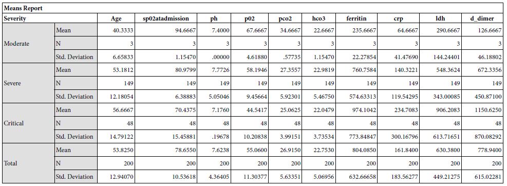
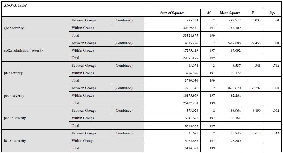
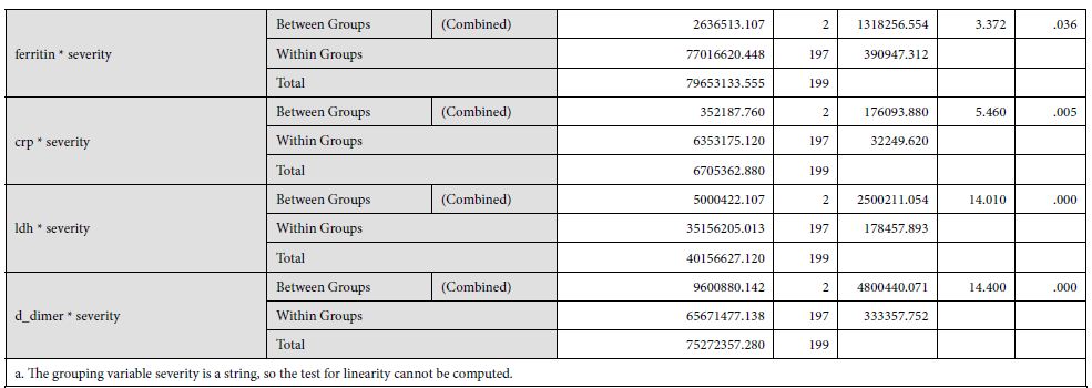
Results: The study yielded 200 participants in which the patients with moderate severity of the disease had a mean age of 40.33±6.65, that with severe disease had a mean age of 53.18±12.1 and critical patients had a mean age of 56.67±14.79. The disease severity is significantly related to increased mean age of the patient (p = 0.050). Mean serum ferritin levels in patients with moderate disease was 235.67±22.27 micrograms per liter, the patients with severe disease had mean value of 760.75±574.63 micrograms per liter and critical patients had a mean ferritin level of 974.10±773.85 micrograms per liter. This revealed that the ferritin levels increased significantly in patients with severe disease
Conclusion: Our findings establish a consistent increase in the levels of D-dimers with increasing severity of the disease, from mild to severe to critical patients. D –Dimers are important predictors of prognosis and disease severity which can be utilized to evaluate the treatment outcomes in COVID-19 infection. Further studies are recommended to find out the cut-off value of D-dimers as a biomarker of disease severity.
Introduction
Covid-19 disease is a global pandemic caused by severe acute respiratory syndrome coronavirus 2 (SARS‑CoV‑2) [1]. It was initially identified in city of Wuhan in December 2019 [2]. World Health Organization declared corona virus as a pandemic on 11 March 2020 [3]. It is a virus of zoonotic origin thought to be transmitted by air borne route. Symptoms of COVID-19 can be relatively non-specific; most common symptoms are fever, dry cough ,sore throat ,shortness of breath, myalgias, abdominal pain ,diarrhea, loss of sense of smell and taste [4]. Approximately one in five patients who become symptomatic become critical and suffer breathing difficulties, persistent chest pain, sudden confusion, difficulty waking, and bluish face or lips. Complications include pneumonia, acute respiratory distress syndrome, sepsis, septic shock, and kidney failure [5]. Covid-19 related complications are associated with high mortality rate.
Researchers all over the world are trying their best to identify its causative factors, patho- physiology and treatment modalities. Retrospective cohort studies carried out in China showed significant mortality and morbidity associated with high D dimers value in admitted patients [6]. COVID related Acute Respiratory Distress Syndrome (ARDS) showed a pro coagulant pattern and this state depicted significant mortality with pulmonary embolism. Covid-19 infection triggered a inflammatory cytokine response which initiated a thrombotic state .It was observed in many studies mortality was reduced by anticoagulation with Low Molecular Weight Heparin (LMWH). The coagulation abnormalities seen in COVID are different from that seen in DIC (sepsis). In DIC, thrombocytopenia is a key finding along with elevated clotting time. However, in cohorts non-surviving patients had an average platelet count and a pro thrombin time which falls within the normal range. It thus may be more likely that local rather than disseminated thrombin generation is at play in COVID-19 patients [7-9].
The main aim of our study was to see the association of D dimers with the prognosis of covid-19. Our study investigated COVID patients and role of D dimers in their mortality and morbidity. There is lack of international & local studies, therefore our study will have a huge impact on researchers and the national data base.
Material & Methods
This Retrospective Cross-sectional study was done at Benazir Bhutto hospital Rawalpindi, which was nominated by Punjab government as COVID Dedicated Unit. Sampling technique used was consecutive sampling. Total sample size obtained was 200 patients. All those patients being admitted in COVID wards during 2 months May- June 2020 were assessed on the basis of D dimers and their 28 day outcome. As d dimers is an easy and inexpensive test was used a screening tool for risk stratification of Covid-19 patients.
Cases of corona virus infection were confirmed by RT-PCR. A patient diagnosed as COVID-19 on the basis of ABI 7500 Real Time RT-PCR detection system after RNA extraction (Qiagen Viral RNA Mini Kit) with internal and external positive controls, using the SARS-CoV-2 protocol.
Inclusion & Exclusion Criteria
Confirmed COVID-19 cases were included in our study where as pregnant women, patients having any hematologic malignancy, chronic liver disease, acute coronary syndrome, surgery or trauma within 30 days and patients without D-dimer testing upon admission were excluded from our study.
Data Collection Technique
Demographic, clinical lab data and outcome (survival or death) was collected form patient records and recorded on self-designed proforma. Disease Severity was be defined as per WHO criteria into moderate, severe, critical with ARDS and Critical with Sepsis/Septic shock. Patients were grouped into two : group A (D-dimer < 500ng/ml) and Group B ( D-dimer ≥ 500ng/ml).
Data Analysis
Data was analyzed via SPSSv25.0. Numerical data was represented as mean and standard deviation. Independent sample t test was used to compare difference of means of numerical variables across severity of the disease according to WHO criteria. Categorical variables were represented as frequencies (%). Distribution of frequencies across severity was compared by Chi-Square test. ROC curve was plotted to determine the cut-off point for D-Dimer to predict mortality.
Ethical Consideration
Ethical approval was solicited from the Institutional Research Forum of Rawalpindi Medical University before securing access to patient data.
Results
The study yielded 200 participants with a mean age of 53.82±12.94 years. On the basis of stratification of severity, the patients with moderate severity of the disease had a mean age of 40.33±6.65, that with severe disease had a mean age of 53.18±12.1 and critical patients had a mean age of 56.67±14.79. The disease severity is significantly related to increased mean age of the patient (p = 0.050). At the time of admission, the patients with moderate disease had a mean SpO2 of 94.67±1.15%, patients with severe disease had a mean SpO2 of 80.79±6.39%, and critical patients had a mean SpO2 of 70.43±15.46%. The mean oxygen saturation at the time of admission decreased with increasing severity (p = 0.000). The patients with moderate disease had a mean arterial partial pressure of oxygen (pO2) of 66.67±6.61 mmHg, patients with severe disease had a mean pO2 of 58.19±9.45 mmHg, and critical patients had a mean pO2 of 44.54±10.21 mmHg. The mean partial pressure of oxygen showed a decline with increasing severity (p = 0.000). Regarding mean arterial partial pressure of carbon dioxide in the patients, the patients with moderate disease had pCO2 of 34.67±6.61 mmHg, patients with severe disease had a mean pCO2 of 27.35±5.92 mmHg, and critical patients had a mean pCO2 of 25.06±3.99 mmHg. The mean partial pressure of carbon dioxide showed a decline with increasing severity (p = 0.002). Mean serum ferritin levels in patients with moderate disease was 235.67±22.27 micrograms per liter, the patients with severe disease had mean value of 760.75±574.63 micrograms per liter and critical patients had a mean ferritin level of 974.10±773.85 micrograms per liter. This revealed that the ferritin levels increased significantly in patients with severe disease. Upon investigating the levels of C-Reactive protein, mean serum CRP levels in patients with moderate disease was 235.67±22.27 mg/L, the patients with severe disease had mean value of 760.75±574.63 mg/L and critical patients had a mean ferritin level of 974.10±773.85 mg/L.
Discussion
Laboratory Hemostasis is believed to provide a very strong evidence in screening, definitive diagnosis and prognosis of many human pathologies [10]. Measuring the levels of D-dimers is one of them. D-dimers are the products of fibrin degradation, which serve as a biomarker in a lot of diseases associated with coagulopathies e.g in coronary artery atherosclerosis, Disseminated intravascular disease and Venous Thromboembolism [11]. D-dimer levels have played a significant role in the evaluation of patients suffering from Community Acquired Pneumonia [12], 2009 novel influenza A (H1N1) [13] and various other members of Coronaviridae family. Covid-19 has also been associated with an increased risk of Venous Thromboembolism [14-15-16]. Hence, the coagulopathy involved in Covid-19 infections can serve as a major determinant of disease prognosis [17]. The levels of D-dimers are consistently elevated in patients suffering from Covid-19 [18-19-20]. In this study, we aimed to explore the association of D-dimer levels with disease severity of Covid-19.
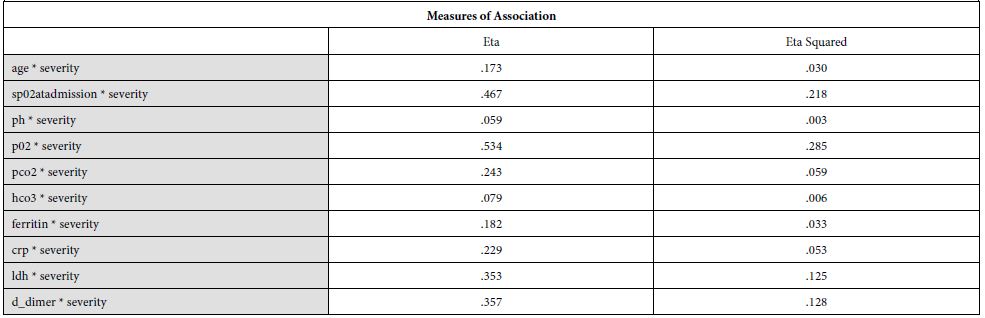
Our findings establish a consistent increase in the levels of D-dimers with increasing severity of the disease, from mild to severe to critical patients [Table 1]. The severity of these patients depended on the duration for which these patients remained in the hospital under care. A strong association was established between these two (Eta sq. 0.128). Many studies concluded the increasing levels of D-dimers to be associated with severity of Covid patients. Huang et al. studies the data of 41 patients and reported a five-fold increase in critical patients (median: 2.4 mg/L; IQR: 0.6–14.4 mg/L) as compared to the non-critical ones (median: 0.5 mg/L; IQR: 0.3–0.8 mg/L; p = 0.004) [21]. Another study was performed by Zhou et al. (16). He reported a nine-fold increase in patients who died of Covid (median: 5.2 mg/L; IQR: 1.5–21.1 mg/L) than in those who survived (median: 0.6 mg/L; IQR: 0.3–1.0 mg/L; p < 0.001). Tand et al. [22] and Wang et al. [23] also had consistent findings as ours. Moreover, irrespective of age, BMI, sex, Hypertension or Diabetes, increased coagulation biomarkers in Covid patients invariably required an increased Oxygen supply, which again can be linked as increased severity in patients having adverse coagulopathies [24].
Table 1: Showing study variables and their severity along with p value.
|
Study variables |
Number
(n) |
Percentage
(%) |
Severity |
p-value |
||||
| Gender | ||||||||
|
Male |
126 | 63 | 1 | 96 | 29 | 126 | 0.496 | |
| Female | 74 | 37 | 2 | 53 | 19 | 74 | ||
| Shortness of Breath | ||||||||
|
Yes |
179 | 89.5 | 2 | 134 | 43 | 179 | 0.429 | |
| No | 21 | 10.5 | 1 | 15 | 5 |
21 |
||
| Fever | ||||||||
|
Yes |
100 | 50.0 | 1 | 77 | 22 | 100 | 0.659 | |
| No | 100 | 50.0 | 2 | 72 | 26 | 100 | ||
| Cough | ||||||||
|
Yes |
46 | 23.0 | 1 | 77 | 22 | 100 | 0.494 | |
| No | 154 | 77.0 | 2 | 72 | 26 | 100 | ||
| Sore Throat | ||||||||
|
Yes |
19 | 9.5 | 0 | 17 | 2 | 19 | 0.282 | |
| No | 181 | 90.5 | 3 | 132 | 46 |
181 |
||
| Diarrhea | ||||||||
|
Yes |
11 | 5.5 | 1 | 6 | 4 | 11 | 0.057 | |
| No | 187 | 93.5 | 2 | 141 | 44 |
187 |
||
| Diabetes Mellitus | ||||||||
|
Yes |
94 | 47.0 | 2 | 62 | 30 | 94 | 0.033 | |
| No | 106 | 53.0 | 1 | 87 | 18 |
106 |
||
| Hypertension | ||||||||
|
Yes |
94 | 47.0 | 0 | 73 | 21 | 94 | 0.212 | |
| No | 106 | 53.0 | 3 | 76 | 27 |
106 |
||
| Ischemic Heart Disease | ||||||||
|
Yes |
37 | 18.5 | 0 | 27 | 10 | 37 | 0.648 | |
| No | 163 | 81.5 | 3 | 122 | 38 |
163 |
||
| Chronic Obstructive Pulmonary Disease | ||||||||
|
Yes |
9 | 4.5 | 0 | 6 | 3 | 9 | 0.755 | |
| No | 191 | 95.5 | 3 | 143 | 45 |
191 |
||
| Asthma | ||||||||
|
Yes |
11 | 5.5 | 0 | 9 | 2 | 11 | 0.810 | |
| No | 189 | 94.5 | 3 | 140 | 46 |
189 |
||
| Rheumatoid Arthritis | ||||||||
|
Yes |
3 | 1.5 | 0 | 3 | 0 | 3 | 0.594 | |
| No | 197 | 98.5 | 3 | 146 | 48 |
197 |
||
| Chronic Kidney Disease | ||||||||
|
Yes |
7 | 3.5 | 0 | 5 | 2 | 7 | 0.914 | |
| No | 193 | 96.5 | 3 | 144 | 46 |
193 |
||
| Hepatitis B/C Infection | ||||||||
|
Yes |
7 | 3.5 | 0 | 6 | 1 | 7 | 0.773 | |
| No | 193 | 96.5 | 3 | 143 | 47 |
193 |
||
| Hypothyroidism | ||||||||
|
Yes |
7 | 3.5 | 0 | 5 | 2 | 7 | 0.913 | |
| No | 193 | 96.5 | 3 | 144 | 46 |
193 |
||
| PCR | ||||||||
|
Positive |
152 | 76.0 | 3 | 108 | 41 | 152 | 0.117 | |
| Negative | 48 | 24.0 | 0 | 41 | 7 |
48 |
||
| Arterial Blood Gases (ABG) Interpretation | ||||||||
|
Normal |
68 | 34.0 | ||||||
| Acute respiratory Failure 1 | 126 | 63.0 | ||||||
|
Acute respiratory Failure 2 |
2 | 1.0 | ||||||
| Compensated/Chronic Respiratory Failure | 4 |
2.0 |
||||||
| Oxygen Flow | ||||||||
|
Normal |
110 | 55.0 | ||||||
| High Flow | 60 |
30.0 |
||||||
|
Low Flow |
30 |
15.0 |
||||||
| Oxygen Support Device | ||||||||
|
NRBM |
108 | 54.0 | ||||||
| Nasal canula | 3 |
1.5 |
||||||
|
BIPAP |
8 | 4.0 | ||||||
| Face Mask | 42 |
21.0 |
||||||
|
Ventilator |
30 | 15.0 | ||||||
| None | 8 |
4.0 |
||||||
| Methylprednisolone Therapy | ||||||||
|
Yes |
101 | 50.5 | 2 | 73 | 26 | 101 | 0.702 | |
| No | 99 | 49.5 | 1 | 76 | 22 | 99 | ||
| Dexamethasone Therapy | ||||||||
|
Yes |
156 | 78.0 | 2 | 73 | 26 | 101 | 0.151 | |
| No | 44 | 22.0 | 1 | 76 | 22 | 99 | ||
| Ivermectin Therapy | ||||||||
|
Yes |
117 | 58.5 | 3 | 98 | 16 | 117 | 0.000 | |
| No | 83 | 41.5 | 0 | 51 | 32 |
83 |
||
| Tocilizumab Therapy | ||||||||
|
Yes |
25 | 12.5 | 0 | 20 | 5 | 25 | 0.692 | |
| No | 175 | 87.5 | 3 | 129 | 43 | 175 | ||
| Heparin Therapy | ||||||||
|
Yes |
177 | 88.5 | 3 | 134 | 40 | 177 | 0.377 | |
| 11.5 | 0 | 15 | 8 | 23 | ||||
| Outcome | ||||||||
|
Expired |
36 | 18.0 | 0 | 0 | 36 | 36 | 0.000 | |
| Improved | 160 | 80.0 | 3 | 148 | 9 |
160 |
||
|
Critical |
4 | 2.0 | 0 | 1 | 3 | 4 | ||
| Severity | ||||||||
|
Moderate |
3 | 1.5 | ||||||
| Severe | 149 |
74.5 |
||||||
|
Critical |
48 |
24.0 |
||||||
The underlying biological plausibility and pathogenesis behind increased D-dimers in Covid-19 can be understood by the disease triggering an inflammatory response. Covid-19 is associated with increased acute phase reactant proteins e.g CRP, as shown in [Table 2] of our findings. Other studies also show a consistent increase in CRP levels with an associated mortality rate of 30 days in coronavirus patients [25]. In the consequence of inflammation, proinflammatory cytokines such as Interleukin 1 (IL-1), Interleukin 6 (IL-6) and tumor necrosis factor-α (TNF-α) are elevated [20]. This results in a cytokine storm that triggers monocytes and macrophages to express tissue factor which leads to thrombin generation [26]. There is also an endothelial damage which results in increased plasma concentrations of tissue-type plasminogen activator (t-PA), upto six-fold increase [27]. This explains the increased levels of D-dimers in Covid-19 patients. Moreover, an accompanied increase in metalloproteinases explains the extracellular matrix modification, resulting in capillary damage and pulmonary edema. The remarkable fibrinolytic profile of Covid patients has also been explained by the studies performed in mice [28]. However, it is noteworthy that increased fibrinolytic profile can still not be translated as DIC or hyper fibrinolytic state. Although coagulopathy may reflect some similar findings, but Covid coagulopathy has a very complex etiology, resulting from intricate interactions between the immune system and coagulation system in the host [29].
Table 2: Showing underlying biological plausibility and pathogenesis behind increased D-dimers in Covid-19.

The ROC curve of our findings for the D-dimer test with severity of Covid diseases is shown in [Figure 1]. The area under the curve (AUC) is 0.699. It can be utilised to determine a definitive cut-off value to support the International Society of Thrombosis and Haemostasis (ISTH) arbitrary definition of raised D-dimers in coronavirus patients as done by Zhang et al [30].
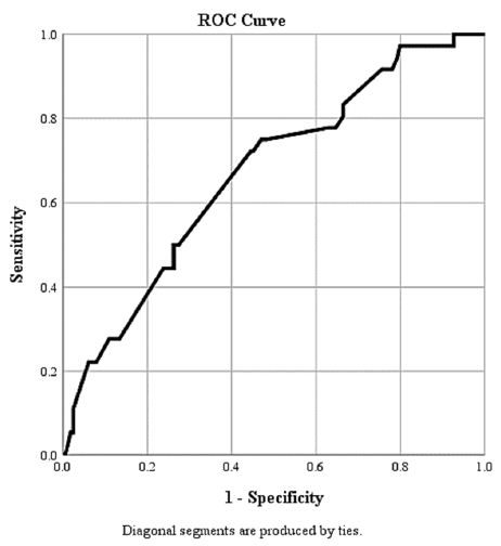
Figure 1: ROC for D-Dimer as a Predictor of Outcome in COVID-19 Infection Area Under the Curve (AUC) is 0.669
Limitations
There are a few limitations in our study that need to be known. Firstly, the burden of the pandemic itself and an emergency situation in Pakistan has hindered the practicality of Cohort, Case-control or Randomized Control Trial- which could have provided a greater pool of Clinical and Lab findings; making even better associations possible. Secondly, we cannot exclude the strong association of confounding factors with coagulopathies- hence a stratified analysis of these confounders can give us a better picture of using D-dimers as a prognostic marker in Covid-19 patients. Moreover, limitations in the measurement of plasma D-dimer concentration may also exist at the level of Laboratory methods and skills involved at human level [31].
Conclusion
COVID-19 infection is characterized by hypercoagulability, inflammation, and multi-organ damage mediated by cytokines. These pathologies are manifested by appearance of several acute phase proteins and inflammatory markers in the serum. The levels of these biomarkers are variable in various stages of COVID-19 infection in relation to severity. The prognosis can be predicted by these serum biomarkers. In this study, D-dimers are measured in patients at various stages of disease severity. D-dimers are important predictors of prognosis and disease severity. These biomarkers can be utilized to evaluate the treatment outcomes in COVID-19 infection. Further studies are recommended to find out the cut-off value of D-dimers as a biomarker of disease severity.
Conflict of Intrest
Nill to disclose
Funding
Nill to disclose
References
- Zu ZY, Jiang MD, Xu PP, et al. (2020) Coronavirus Disease 2019 (COVID-19): A Perspective from China. Radiology Aug;296(2):E15-E25. doi: 10.1148/radiol.2020200490. Epub 2020 Feb 21. [crossref]
- Sahin AR, Erdogan A, Agaoglu PM, et al. (2020) 2019 novel coronavirus (COVID-19) outbreak: a re-view of the current literature. EJMO 4(1):1_7.
- https://www.who.int/news/item/23-01-2020-statement-on-the-meeting-of-the-international-health-regulations-(2005)-emergency-committee-regarding-the-outbreak-of-novel-coronavirus-(2019-ncov)
- Hopkins C. “Loss of sense of smell as marker of COVID-19 infection”. Ear, Nose and Throat surgery body of United Kingdom. Retrieved 28 March 2020.
- Interim Clinical Guidance for Management of Patients with Confirmed Coronavirus Disease (COVID-19)”. S. Centers for Disease Control and Prevention (CDC) Retrieved 11 April 2020. https://www.cdc.gov/coronavirus/2019-ncov/hcp/clinical-guidance-management-patients.html.
- Lippi G, Favaloro EJ (2020) D-dimer is Associated with Severity of Coronavirus Disease 2019: A Pooled Analysis. Thromb Haemost May;120(5):876-878. doi: 10.1055/s-0040-1709650. Epub 2020 Apr 3. [crossref]
- Tang N, Li D, Wang X, et al. (2020) Abnormal coagulation parameters are associated with poor prognosis in patients with novel coronavirus pneumonia. J Thromb Haemost Apr;18(4):844-847. doi: 10.1111/jth.14768. Epub 2020 Mar 13. [crossref]
- Ranucci M, Ballotta A, Di Dedda U, et al. (Jul. 2020) The procoagulant pattern of patients with COVID-19 acute respiratory distress syndrome. J Thromb Haemost 18(7):1747-1751. doi: 10.1111/jth.14854. Epub 2020 May 6. [crossref]
- Wang T, Chen R, Liu C, et al. (May 2020) Attention should be paid to venous thromboembolism prophylaxis in the management of COVID-19. Lancet Haematol 7(5):e362-e363. doi: 10.1016/S2352-3026(20)30109-5. Epub 2020 Apr 9. [crossref]
- Lippi G, Favaloro EJ (Jun. 2018) Laboratory hemostasis: from biology to the bench. Clin Chem Lab Med 27;56(7):1035-1045. doi: 10.1515/cclm-2017-1205. [crossref]
- Soomro AY, Guerchicoff A, Nichols DJ, et al. (Jul. 2016) The current role and future prospects of D-dimer biomarker. Eur Heart J Cardiovasc Pharmacother 2(3):175-84. doi: 10.1093/ehjcvp/pvv039. Epub 2015 Sep 27. [crossref]
- Chalmers J.D., Singanayagam A., Scally C., et al. (2009) Admission D-dimer can identify low-risk patients with community-acquired pneumonia. Emerg. Med. 53:633–638. doi: 10.1016/j.annemergmed.2008.12.022. [crossref]
- Wang Z.F., Su F., Lin X.J., et al. (2011) Serum D-dimer changes and prognostic implication in 2009 novel influenza A(H1N1). Res 127:198–201. doi: 10.1016/j.thromres.2010.11.032. [crossref]
- Helms J., Tacquard C., Severac F., et al. (2020) High risk of thrombosis in patients with severe SARS-CoV-2 infection: A multicenter prospective cohort study. Intensive Care Med 46:1089–1098. doi: 10.1007/s00134-020-06062-x. [crossref]
- Leonard-Lorant I., Delabranche X., Severac F, et al. Acute Pulmonary Embolism in COVID-19 Patients on CT Angiography and Relationship to D-Dimer Levels. Radiology. 2020:201561. doi: 10.1148/radiol.2020201561. [crossref]
- Fauvel C., Weizman O., Trimaille A., et al. (2020) Pulmonary embolism in COVID-19 patients: A French multicentre cohort study. Heart J. 41:3058–3068. doi: 10.1093/eurheartj/ehaa500. [crossref]
- Tang N., Li D., Wang X., et al. (2020) Abnormal coagulation parameters are associated with poor prognosis in patients with novel coronavirus pneumonia. Thromb. Haemost. 18:844–847. doi: 10.1111/jth.14768. [crossref]
- Thachil J (2020) All those D-dimers in COVID-19. Thromb. Haemost. doi: 10.1111/jth.14939. [crossref]
- Lippi G. (2020) Favaloro E.J. D-dimer is Associated with Severity of Coronavirus Disease 2019: A Pooled Analysis. Haemost. 120:876–878. doi: 10.1055/s-0040-1709650. [crossref]
- Huang C, Wang Y, Li X et al. (2020) Clinical features of patients infected with 2019 novel coronavirus in Wuhan, China. Lancet 395(10223):497–506. [crossref]
- Zhou F, Yu T, Du R et al. (2020) Clinical course and risk factors for mortality of adult inpatients with COVID-19 in Wuhan, China: a retrospective cohort study. Lancet S0140-6736(20)30566-3. [crossref]
- Tang N, Li D, Wang X, et al. (2020) Abnormal coagulation parameters are associated with poor prognosis in patients with novel coronavirus pneumonia. J Thromb Haemost Doi: 10.1111/jth.14768. [crossref]
- Wang D, Hu B, Hu C, et al. (2020) Clinical characteristics of 138 hospitalized patients with 2019 novel coronavirus-infected pneumonia in Wuhan, China. JAMA Doi: 10.1001/jama.2020.1585. [crossref]
- https://onlinelibrary.wiley.com/doi/10.1111/jth.15067
- Huang I, Pranata R, Lim MA, et al. (Jan.-Dec. 2020) C-reactive protein, procalcitonin, D-dimer, and ferritin in severe coronavirus disease-2019: a meta-analysis. Ther Adv Respir Dis 14:1753466620937175. doi: 10.1177/1753466620937175. [crossref]
- Levi M, Thachil J. (2020) Coronavirus disease 2019 coagulopathy: disseminated intravascular coagulation and thrombotic microangiopathy-either, neither, or both. Semin Thromb Hemost 46:781–784. doi: 10.1055/s-0040-1712156. [crossref]
- Liu ZH, Wei R, Wu YP, et al. (2005) Elevated plasma tissue-type plasminogen activator (t-PA) and soluble thrombomodulin in patients suffering from severe acute respiratory syndrome (SARS) as a possible index for prognosis and treatment strategy. Biomed Environ Sci BES 18:260–264. [crossref]
- Gralinski LE, Bankhead A, Jeng S, et al. (2013) Mechanisms of severe acute respiratory syndrome coronavirus-induced acute lung injury. mBio 4:e00271–e313. doi: 10.1128/mBio.00271-13. [crossref]
- Iba T, Levy JH, Levi M, et al. (Sep. 2020) Coagulopathy of Coronavirus Disease 2019. Crit Care Med 48(9):1358-1364. doi: 10.1097/CCM.0000000000004458. [crossref]
- Zhang L et al. (2020) D-dimer levels on admission to predict in-hospital mortality in patients with Covid-19. Journal of Thrombosis and Haemostasis 18, 1324–1329. [crossref]
- Hardy M., Lecompte T., Douxfils J, et al. (2020) Management of the thrombotic risk associated with COVID-19: Guidance for the hemostasis laboratory. J. 18:17. doi: 10.1186/s12959-020-00230-1. [crossref]