Author Archives: author

Formulation of Rivastigmine, a Liquid Drug Substance, for Use in a Simulating Study of Hollow Microstructured Transdermal Delivery System

DOI: 10.31038/JPPR.2020333

Abstract

Rivastigmine, used in the treatment of Alzheimer’s Disease, is in liquid state at controlled room temperatures. This project was aimed at developing a 0.5-mL isotonic liquid containing rivastigmine with the choice of 0.9% NaCl or 5% Dextrose Solutions for Injection as a simulating study to formulate a liquid dosage form per description of 3M hollow microneedles (https://multimedia.3m.com/mws/media/1004089O/solid-microstructured-transdermal-system-smts-sell-sheet.pdf). The surfactants were compared among Span 20, Span 80, Tween 40 and Tween 80 with benzyl alcohol or chlorobutanol as a preservative. Those formulations which formed microemulsions were further studied for stability at 4°C and 25°C up to one month. HPLC confirmed that there were no drug losses among the four microemulsions. Based on zeta potential and particle size analysis, Tween 80 with benzyl alcohol in 0.9 % NaCl is the best project formulation.

Keywords

Benzyl alcohol, chlorobutanol, Hollow Microstructured Transdermal System (hMTS), microneedles, rivastigmine, Tween and Span

Introduction

Alzheimer’s disease is an irreversible, progressive neurodegenerative disorder subsequently becoming a common cause of death [1]. Alzheimer’s is the most common cause of dementia affecting an estimated 5.8 million people in the United States [1]. In 2018, the approximate cost of caring for people with Alzheimer’s disease and other dementias was $290 billion USD, making it a huge economic burden for both patients’ families and our society and leading to a major public health problem. It is a huge economic burden for patients’ families and our society. Unfortunately, there has not been an effective treatment for Alzheimer’s disease thus far. One of the reasons is that the exact mechanism of disease development is still unclear. Acetylcholinesterase inhibitors such as donepezil, rivastigmine and galantamine, and N-methyl D-asparate receptor antagonist, and memantine are therapeutic agents. Among them, rivastigmine has the advantage of inhibiting both acetylcholinesterase (AChE) and butyrylcholinesterase (BuChE). It is also superior to the aforementioned other drugs in having two US FDA approved commercial dosage forms, that is oral capsules and transdermal patches (Table 1) [2,3]. Unfortunately, nausea and vomiting have been reported by patients taking rivastigmine oral dosage form [4]. Transdermal delivery system has a better tolerability and more efficacy compared to oral capsules [5] and enables patients who have difficulties in swallowing to take medicine more easily, and less frequently (once daily, Table 1b) [6]. However, it was reported that transdermal patch may cause skin irritation when a 24-h patch is worn. Therefore, this study focuses on the feasibility of formulating rivastigmine for use of microneedle administration and formulation characterizations. Microneedle has been gathering attention on their merits, including shorter time to reach C_max and penetrating more drugs, especially macromolecules, than the transdermal patch dosage form [7].

Table 1: Rivastigmine dosage forms on the market: (a) oral capsules, and (b) extended release transdermal films [2,3].

(a) Oral capsules

Strength	Manufacturers	Applicant Holder
EQ 1.5, 3, 4.5, 6 mg BASE	Brand name product	Novartis
EQ 1.5, 3, 4.5, 6 mg BASE	Generic products	Alembic; Apotex; Aurobindo; Cadila; Chartwell; Dr. Reddy’s; Macleods; Orchid; Sun; Watson

(b) Extended release transdermal film

Strength

Manufacturers

Applicant Holder

4.6, 9.5, 13.3 mg/24 h

Brand name product

Novartis

4.6, 9.5, 13.3 mg/24 h

Generic products

Alvogen malta operations;

Amneal; Mylan; Zydus

Microneedles devise a pain-free penetration feature (minimally invasive device which pierces through the stratum corneum without touching the nerve endings and capillaries). Its other merits are avoidance of the first-pass, improvement of skin permeability and permeation, the delivery of both small and large molecules, achieve stable plasma concentrations for up to 7 days and possibly improvement of bioavailability. There are four subtypes of microneedles: solid, coated, dissolving, and hollow [8-10].

Colloidal Dispersions, Emulsions and Microemulsions

Colloids are heterogeneous mixture systems. Colloidal dispersion is characterized by their particle sizes and shapes. A particle size ranged between 1 nm and 1 μm makes the properties of colloids fall between solution and suspensions. Whether their particles are small enough to separate on standing or are large enough to scatter light (a phenomenon called Tyndall effect, which makes the liquid’s appearance cloudy or opaque) depends on the particle size. Therefore, colloidal dispersions are further divided into molecular colloids (solutions), association colloids and dispersion colloids [11]. Emulsions are composed of two or more immiscible liquids and suitable emulsifying agent(s), which appear milky and nontransparent because of the different optical refraction of the components. Depending on the hydrophilic and lipophilic characters, emulsions may be divided into oil in water (O/W) and water in oil (W/O) subtypes. In addition to these, multiple phases of emulsions exist as W/O/W and O/W/O microemulsions. Emulsions are kinetically stable but thermodynamically unstable based on their dispersed state and the corresponding high interfacial energy. On the other hand, microemulsions are fundamentally different from emulsions in terms of appearance, structure, and properties, which are considered between micellar solution and emulsions. Their appearances vary from transparent to opalescent, moderately viscous, and optically isotropic. Microemulsions are thermodynamically stable [11,12].

Materials

Rivastigmine (1 g and 0.5 g HY-17368 in two separate orders; liquid state in controlled room temperature) was obtained from MedChem Express (Monmouth Junction, NJ). 5 % Dextrose (also known as D5W, Lot J4J577) and 20 mL syringes were acquired from Cardinal Health (Dublin, OH). Sodium chloride (Lot: 284929), Tween 40 (polyxyethylene sorbitan monopalmitate, Lot: D5ZONHK, TGI Tokyo, Japan), methanol and 0.2 micron VWR syringe filters were ordered from VWR International (Randor, PA). Span 20 (Sorbitan monolaurate, Lot: C1885020), Span 80 (sorbitan monooleate, Lot: C182545), Tween 80 (polysorbate, Lot: C188508), benzyl alcohol (Lot: C171703), chlorobutanol, and sodium phosphate dibasic were bought from PCCA (Houston, TX).

Methods

Determination of High Performance Liquid Chromatographic (HPLC) Column

USP43-NF38 2020 recommended to assay rivastigmine and its tartrate salt by using Symmetry C18, Nova Pak C18, and Spherisorb C8 columns [13]. Buffer was first prepared as 8.9 g/L of dibasic sodium phosphate dihydrate in water (0.05 M). Mobile phase was the mixture of methanol and Buffer (0.05M sodium phosphate dibasic) in 58:42 v/v ratio. The solution was let cool to controlled room temperature before the pH adjustment to the value of 8.45 using phosphoric acid. The LC assay conditions were flow rate of 1.0 mL/min, and column temperature at 40°C. The detection wavelength was chosen at 214 nm for all study LC columns with run time at 20 minutes initially. When no impurities were seen, the run time was reduced to 15 minutes or shorter to avoid the generation of biohazard wastes from the prolonged use of mobile phase containing methanol.

Standard Curve

Ten mL of rivastigmine (which density is 1.0 g/mL) initially placed in a volumetric flask to determine its weight. A sufficient amount of the mobile phase was then added to make it into 10 mL as the stock solution, which has a concentration of 1 mg/mL (because the density of rivastigmine is 1 g/mL). This stock solution was further diluted 5-fold with mobile phase each time for sequentially six times with the eighth sample only being diluted two-fold from the seventh sample. One mL of each was transferred into a HPLC vial for assay injection. Accuracy is determined based on how close a measured value is to the actual (true) value. One of the actual (true value) may rely on the use of USP Reference Standard for comparison. Precision is determined based on how close the measured values are to each other. Since Rivastigmine USP Reference Standard was not available for the free base form to report Accuracy (but available as Rivastigmine Tartrate). This project reported the Precision instead. The HPLC conditions were as the follows: wavelength at 214 nm; flow rate 1.0 mL/min; run time 12 min; column temperature 40°C.

Formulation Preparation

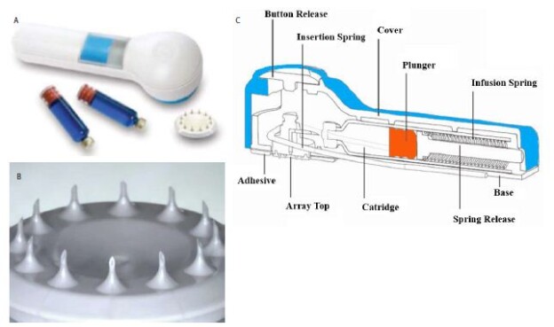
3M Hollow Microstructured Transdermal System (hMTS) is an integrated device containing actuator, glass injection cartridge, delivery spring, adhesive, hollow microstructured array and application spring with information available at 3M, St. Paul, MN [12]. Each glass cartridge may house 0.5 mL to 2 mL of intradermal delivery solution (Figure 1a and 1b). In this project, 4.6 μL of rivastigmine (that is 4.6 mg) was selected to develop into 0.5 mL of liquid dosage form as a single dose. As aforementioned, rivastigmine is in liquid state at controlled room temperature, its density is 1.0 g/mL. Therefore, rivastigmine was measured by volume, instead of weight in this project. Suitable excipients such as solution for injection, surfactant and preservative were added into the final volume of 0.5046 mL, which is within the glass cartridge capacity between 0.5 mL to 2 mL. The selection of excipients such as Solutions for Injection, surfactants, and preservatives are briefly described as follows. Isotonic 0.9% saline and 5% dextrose (D5W) were chosen as Solutions for Injection. Since rivastigmine is lipophilic and in liquid state at controlled room temperature (23 ± 2°C), four surfactants (Span 20; Span 80; Tween 40 and Tween 80 (Figure 2) were added respectively to check compatibility. In addition, two preservatives (benzyl alcohol or chlorobutanol) were included. Each formulation in the saline group was composed of 0.9 g of NaCl, 5.0 g of surfactants and 1.0 g of benzyl alcohol (or 0.5g of chlorobutanol) in 100 mL final volume. The D5W group contained 5.36 g of surfactants, 1.0 g of benzyl alcohol (or 0.5 g of chlorobutanol) with sufficient amount of D5W in the total of 100 mL final volume. After mixing, the degree of transparency vs. cloudiness of all formulations were visually observed to determine candidacy for further testing. Rivastigmine 0.92 mL was taken and mixed with each 100 mL of liquid to assess particle size, zeta potential and conduct HPLC.

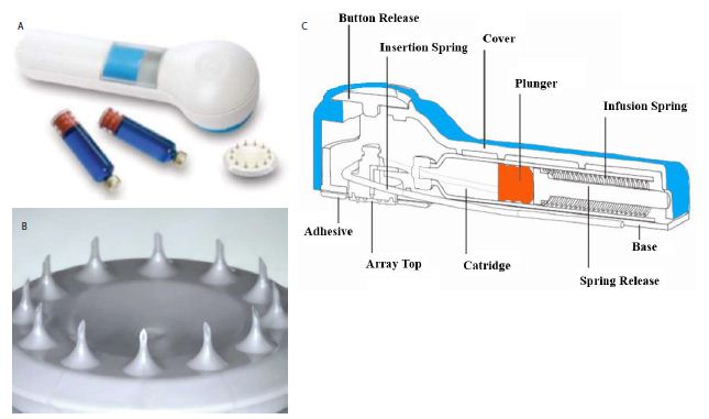
Figure 1: Hollow Microneedle Transdermal System (hMTS): (a) 3M device, (b) scheme showed the inside view of the integrated device, and (c) polymer microneedle array with 12 hollow microneedles, each approximately 1500 µm [12].

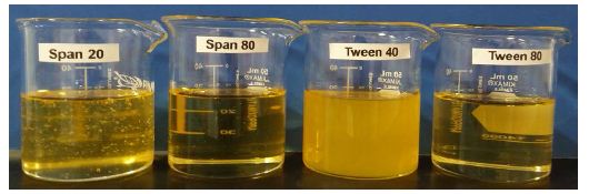
Figure 2: The appearance of surfactants from left to right: Span 20 (HLB 8.6), Span 80 (HLB 4.0), Tween 40 (HLB 15.6) and Tween 80 (HLB 15.0).

Visual Characterization

The miscibilities of resultant formulations after rivastigmine mixed with one of the two Solutions for Injection, one of the four surfactants and one of the two preservatives were visually observed.

Particle Size Analysis and Zeta Potential

Rivastigmine (9.2 μL, density 1 g/mL) was added to the aforementioned different blank formulations into the total volume of 2 mL for each. The formulations were analyzed by the NanoBrook 90 Plus Particle Sizer. The refractive indexes of rivastigmine, Span 20, Tween 40, Tween 80, benzyl alcohol, and chlorobutanol used in particle size analysis were 1.518, 1.474, 1.470, 1.473, 1.539, and 1.491, respectively (Refractive index of a medium is the ratio of the speed of light in vacuum to the speed of light in the medium. Therefore, it has no units). The zeta potentials of formulations were analyzed using NanoBrook 90 Plus Zeta Potential Reader.

One-Month Stability Study

Each formulation sample containing 4.6 μL of rivastigmine (equivalent to 4.6 mg) was subject to HPLC assay as Time 0 samples. The LC method was adopted from USP-NF 2020 [13]. One half mL of this liquid plus 4.6 μL (4.6 mg) of rivastigmine was then taken into an amber vial and crimped with an aluminum cap (as a single dose) and stored at 4°C and 25°C respectively (n = 3) for one month prior to HPLC assay to determine the drug loss and compare the stabilities among formulation candidates.

Statistics

AUCs obtained from HPLC were statistically assessed by one way or two way ANOVA tests when normality and equal variance were met. Kruska-Wallis test was used if normality and equal variance were not met. Tukey as postdoc was used to compare the three groups. Population differences are considered significant at P < 0.05.

Results

Visual Observation

When using D5W as the Solution for Injection and mixed with one of the four surfactants, the Span 20 group looked homogeneous, but Span 80 appeared as heterogeneous. Tween 40 formed a yellowish clear solution. Tween 80 was a pale yellowish clear solution. Therefore, Span 80 was excluded from further experiments. Next, one of the two preservatives was added into these formulations. Preservative (either benzyl alcohol and chlorobutanol) in Span 20 formed milky microemulsion (Table 2). Benzyl alcohol with Tween 40 resulted in colloidal dispersion, while chlorobutanol formed microemulsion. Like Tween 40, chlorobutanol with Tween 80 formed microemulsion but benzyl alcohol had colloidal dispersion. Using 0.9 % NaCl for Solution for Injection, in contrast with D5W, Span 20 and Span 80 were heterogeneous and immiscible. From these results, they were eliminated from the formulation. Tween 40 in 0.9% NaCl was a yellowish clear solution. When benzyl alcohol was added as a preservative, it formed yellowish colloidal dispersion, while chlorobutanol formed precipitations. Tween 80 in 0.9% saline was also a clear solution. When either preservative was added to Tween 80, they formed clear microemulsion.

Table 2: Miscibilities of surfactants and preservatives in D5W or 0.9% NaCl Solution.

Surfactant	Preservative	D5W	0.9% NaCl
Span 20	Benzyl Alcohol	Emulsion	Non-miscible
Span 20	Chlorobutanol	Emulsion	Non-miscible
Span 80		Non-miscible	Non-miscible
Tween 40	Benzyl Alcohol	Colloidal dispersion	Colloidal dispersion
Tween 40	Chlorobutanol	Microemulsion	Precipitation
Tween 80	Benzyl Alcohol	Colloidal dispersion	Microemulsion
Tween 80	Chlorobutanol	Microemulsion	Microemulsion

Particle Size and Zeta Potential Analyses

Span 20 with each preservative in D5W, Tween 80 with chlorobutanol in D5W and Tween 80 with each preservative in 0.9% NaCl were good candidates only in terms of particle sizes (Table 3). Among D5W, Tween 40 was significant different with Span 20 and Tween 80. However, there was no significant difference by using one or the other preservatives. Within benzyl alcohol in D5W, Span 20 and Tween 40 showed significantly different. Nevertheless, Span 20 and Tween 80 or Tween 40 and Tween 80 showed no difference. Furthermore, within chlorobutanol, between Tween 40 and Span 20 or Tween 80 showed a significant difference. Among the sample groups made of 0.9 % NaCl as Solution for Injection, there is no significant difference neither caused by surfactants nor by preservatives. Tween 80 with chlorobutanol in D5W and Tween 80 with either preservative in 0.9% NaCl can especially be considered as good candidates at time zero. Zeta potentials were also showed in the first right column of Table 3. There was no significant difference in terms of which surfactant or preservative was used in D5W or 0.9% NaCl. This suggests the stabilities of all formulation were similar at time zero.

Table 3: Particle sizes and Zeta potentials of six formulas using D5W as Solution for Injection and three formulas using 0.9% NaCl as Solution for Injection.

(a) D5W as Solution for Injection

Surfactant	Preservative	Particle Size (nm) Mean ± SD	Zeta Potential (mV)
Rivastigmine in D5W alone		434.27 ± 74.90	–
Span 20	Benzyl Alcohol	105.08 ± 25.53	-2.40 ± 5.85
Span 20	Chlorobutanol	148.67 ± 60.42	-4.49 ± 9.67
Tween 40	Benzyl Alcohol	6356.20 ± 6314.59	-4.90 ± 1.26
Tween 40	Chlorobutanol	7186.41 ± 5069.88	-2.14 ± 3.10
Tween 80	Benzyl Alcohol	1749.11± 1902.47	-5.88 ± 0.62
Tween 80	Chlorobutanol	10.33 ± 0.17	-1.31 ± 4.77

(b) NaCl as Solution for Injection

Surfactant	Preservative	Particle Size (nm) Mean ± SD	Zeta Potential (mV)
Rivastigmine in 0.9% NaCl alone 360.93 ± 16.68			–
Tween 40	Benzyl Alcohol	13063.80 ± 13634.23	-4.13 ± 6.75
Tween 80	Benzyl Alcohol	12.74 ± 0.17	10.54 ± 16.86
	Chlorobutanol	11.49 ± 0.10	5.46 18.06

HPLC Assay

Column Selections and Standard Curve Linearity Range

Three LC columns (Symmetry C18, Nova Pak C18, and Spherisorb C8) were evaluated in this project. The tailing factors of column kinetics showed that Symmetry C18 was the best column to assay both rivastigmine and its tartrate salt form. The limit of detection of rivastigmine dissolved in mobile phase, and assayed by HPLC according to the method described in Section 5.5 was 0.00032 μL (0.0000320 mg/mL). The limit of quantification was 0.00064 μL (0.0000640 mg/mL). The linearity ranged from 0.000032 mg/mL to 1.0 mg/mL.

The AUC of the formulations which were compounded with different combinations of Solutions for Injection, surfactants and preservatives were assayed and converted into concentrations by applying with an established standard curve. In the group of using D5W as the Solution for Injection, whether the preservative was benzyl alcohol or chlorobutanol, the sample containing Span 20 had a significantly low concentration than those containing Tween 40 and Tween 80 (n = 4, p < 0.01, Figure 3a). There was no difference between either preservative (benzyl alcohol and chlorobutantol) whether the surfactant was Span 80, Tween 40 or Tween 80 (Figure 3a). When 0.9% NaCl solution was used as the solution for injection, there were no differences between Tween 40 and Tween 80 as surfactant while benzyl alcohol was the preservative (Figure 3b). Also, when Tween 80 was used as the surfactant, there was also no difference in using either preservative. The formulation containing benzyl alcohol and Tween 40 was not different to the formulation containing chlorobutanol and Tween 80 in 0.9% NaCl (n = 3, p > 0.05, Figure 3b).

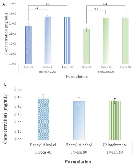
Figure 3: The rivastigmine concentrations of time 0 formulation candidates after chromatographic AUC being converted into concentrations using standard curves: (a) they were differed when D5W was used as the Solution for Injection; while (b) there was no differences when 0.9% NaCl solution was used as the solution for injection. (**p < 0.01, and ***p < 0.001).

One-Month Stability Study

Table 2 showed four of the studied formulations formed into microemulsion. They were further followed up with a stability study at 4°C and 25°C. They were Tween 40 and Tween 80 with chlorobutanol in D5W, and Tween 80 with either chlorobutanol or benzyl alcohol in 0.9% NaCl. When the samples were assayed by HPLC for drug content, there was no significant difference between time 0 and one-month in the metal-cap sealed glass vial samples stored at 4°C and 25°C, respectively (Table 4).

Table 4: The Concentration of Each Formulation at Time 0 and Stored at 4 and 25°C.

Solution for Injection	Surfactant	Preservative	Mean ± SD (n = 3)
Solution for Injection	Surfactant	Preservative	Time 0	4°C	25°C
D5W	Tween 40	Chlorobutanol	0.5165 ± 0.06047	0.5178 ± 0.06480	0.5537 ± 0.06496
D5W	Tween 80	Chlorobutanol	0.4655 ± 0.03859	0.4571 ± 0.04455	0.4693 ± 0.03319
0.9 % NaCl	Tween 80	Benzyl Alcohol	0.4358 ± 0.01938	0.4472 ± 0.00303	0.4424 ± 0.01940
0.9 % NaCl	Tween 80	Chlorobutanol	0.4519 ± 0.01719	0.4490 ± 0.00949	0.4539 ± 0.01468

After One-Month

Discussion

The stability test performed by EMEA was for up to 5 years reported that rivastigmine free base is very sensitive to oxidation, moisture and heat [14]. Degradation is accelerated by the influence of heat. Therefore, it is recommended to be stored at 5 ± 3°C with protection from light and with protective gas [14]. Although the commercial Exelon Rivastigmine Patches also used free base drug, and the FDA approved labels indicated that they may be stored at controlled room temperature, perhaps it is because this commerical patch is packaged in aluminum pouch with an internal polymer coat and external composite printable surface. In our study, we compared the product concentrations at Time 0 and after one month and found no drug loss threatened by oxidation and moisture whether the formulations were stored at 4°C or 25°C. It was because our formulation was packed in metal-cap sealed glass vials prior to being subject to each storage temperature. Since the product of this project is in liquid form (unlike the transdermal patches and oral capsules which are solids), it is suggested that the long-term storage temperature be studied.

Conclusion

When the rivastigmine concentrations among the three surfactants (Span 20, Tween 40 and Tween 80) using benzyl alcohol as the preservative in D5W were compared, Span 20 was significantly different from Tween 40 (p < 0.01). It was also different from Tween 80 (p < 0.01), while Tween 40 and Tween 80 were no different (p = 0.981). This identified that Span 20 is not a suitable surfactant. The same results were acquired when using chlorobutanol as the preservative in D5W. Span 20 was different from Tween 40 (p < 0.001) and Tween 80 (p < 0.001), while Tween 40 and Tween 80 were no different (p = 0.996). Therefore, rivastigmine is not emulsifiable by Span 20 whether the continuous phase is D5W or 0.9% NaCl. Microneedle dosage form is pain-free, minimal invasive and can be administered by health care professionals in clinics and hospital settings, trained home care personnel, or patients themselves at home. This is due to the short injection time to administer 0.5 to 2 mL without having to use a battery or electrical power (Figure 1a and 1b). Syringe filtration of 0.2 micron was applied to obtain the required sterilization of project formulations. Vacuum filtration may be tested as the first sterilization strategy in scale up due to the small volume per dose before studying another method. Future investigation can also focus on whether a preservative in the formulation of this single dose sealed product can be omitted. In the dermis dendritic cells function as immune system responses. Therefore, there will be great potential to deliver vaccines or large molecules using different subtypes of microneedles into the dermis, especially for pediatric, geriatric and other special needs patient populations.

References

Alzheimer’s Association (2019) Alzheimer’s Disease Facts and Figures. Alzheimers Dement 17-57.
https://www.accessdata.fda.gov/scripts/cder/ob/search_product.cfm (Accessed Nov 22, 2020).
Exelon Scientific Discussion. Available at: https://www.ema.europa.eu/en/documents/scientific-discussion-variation/exelon-h-c-169-x-0038-epar-scientific-discussion-extension_en.pdf (accessed Nov 22, 2020).
Birks JS, Chong LY and Grimley Evans J. (2015). Rivastigmine for Alzheimer’s disease. Cochrane Database Syst Rev. [crossref]
Cummings J, Lefèvre G, Small G, Appel-Dingemanse S (2007) Pharmacokinetic rationale for the rivastigmine patch. Neurology [crossref]
Sadowsky CH, Micca JL, Grossberg GT, Velting DM (2014) Rivastigmine from capsules to patch: therapeutic advances in the management of Alzheimer’s disease and Parkinson’s disease dementia. Prim Care Companion CNS Disord. [crossref]
Donnelly RF, Singh TRR, Morrow DIJ, Woolfson MAD (2012) Microneedle-Mediated Transdermal and Intradermal Drug Delivery. Wiley.
Dharadhar S, Majumdar A, Dhoble S and Patravale V (2019) Microneedles for transdermal drug delivery: a systematic review. Drug Development and Industrial Pharmacy 45: 188-201. [crossref]
Larraneta E, Lutton RE, Woolfson DA and Donnelly RF (2016). Microneedle arrays as transdermal and intradermal drug delivery systems: Materials science, manufacture and commercial development. Materials Science and Engineering R 104: 1-32.
Corrie SR, Kendall MAF (2017) Transdermal Drug Delivery. In: Hillery A, editor. Drug Delivery: Fundamentals and Applications, CRC Press, pg: 225-226.
3: Physical and Physicochemical Principles of Drug Formulation, and Ch. 18 Emulsions. (2018). In: Fahr A, Voigt’s Pharamaceutical Technology . Wiley, pg: 41-42, 549-550.
https://multimedia.3m.com/mws/media/1004089O/solid-microstructured-transdermal-system-smts-sell-sheet.pdf (Accessed Nov 22, 2020)
S. Pharmacopeial Convention (2020) USP Monographs: Rivastigmine. In: USP43-NF38. Rockville MD: U.S. Pharmacopeia, pg: 3922.
Scientific Discussion (2007). London: EMEA. https://www.ema.europa.eu/en/documents/scientific-discussion-variation/exelon-h-c-169-x-0038-epar-scientific-discussion-extension_en.pdf (Accessed Nov 22, 2020).

Incidence and Factors of Prolonged Postoperative Ileus in Gastric Cancer Surgery

Leave a reply

DOI: 10.31038/CST.2021612

Abstract

Objective: Prolonged Postoperative Ileus (PPOI) is a common complication after abdominal surgery, but data about incidence and risk factors of PPOI for patients with gastric cancer are rare. We sought to investigate the incidence and related incidental factors of PPOI.

Methods: A retrospective cohort study was carried out using a registry database consecutively collected from June 2016 to October 2016. The incidence and incidental factors of PPOI after gastric cancer surgery were calculated and analyzed.

Results: There were 22 patients diagnosed with PPOI. The incidence of PPOI after gastric cancer surgery was 26.5%. There were significant differences in the PPOI among ages, postoperative body temperature, postoperative opioid agents use (Dezocine) (P<0.05). Logistic regression analysis results showed that the age ≥65 years, postoperative temperature ≥38℃, the use of Dezocine after surgery were the independent risk factors of PPOI after gastric cancer surgery.

Conclusion: The occurrence of PPOI after gastric cancer surgery has great relationship with age, postoperative temperature, the use of Dezocine after surgery. We may accelerate the course of convalescence by strengthening the management of perioperative periodandtaking reasonable measures to against the risk factors.

Keywords

Gastric cancer, Prolongedpostoperative ileus, Incidental factor

Prolonged Post-Operative Ileus (PPOI) is an aberrant pattern of gastrointestinal motility, most frequently occurring after abdominal surgery. The clinical manifestations include abdominal pain, nausea, vomiting, moderate to severe sick, intolerable of a solid diet and a delayed passage of flatus and stool, which usually resolves spontaneously within 2 to 3 days [1,2]. If the symptoms persist for more than 4 days, Prolonged Postoperative Ileus (PPOI) is defined [3]. PPOI hampers the patients’ recovery, increases postoperative morbidity and leads to longer length of hospital stay [4]. Understanding the incidence and factors of PPOI can help clinicians take effective measures to reduce the incidence of PPOI, and ultimately achieve rapid recovery of patients. This study retrospectively collected the clinical information of gastric cancer patients who received surgical treatment in our department, analyzed the related factors of PPOI occurrence, in order to take targeted prevention and treatment measures.

Materials and Methods

1. Study Population

A retrospective cohort study was carried out using a PPOI registry database consecutively collected between June 2016 and October 2016 in Chinese PLA General Hospital. Among them, 62 were male and 21 were female, the ratio of male to female was about 3:1, they were between 39 and 89 years old , and the average age was (60.1 ± 11.0) years . Among them, 34 cases underwent total gastrectomy, 40 cases underwent distal gastrectomy and 9 cases underwent proximal gastrectomy.

2. Diagnosis of PPOI

The definition of PPOI was adopted from the results of a systematic review and global survey [3]. The validity of this concept was universally accepted by a variety of investigators [5-8]. Accordingly, diagnoses of PPOI were identified if two or more of following events after day 4 postoperatively: (a), nausea or vomiting; (b) inability to tolerate an oral diet over the prior 24 hour; (c) absence of flatus over the prior 24 hours; (d) abdominal distension; (e) radiologic confirmation.

3. Method

The clinical data of 83 patients with gastric cancer were collected, including gender, age, BMI index, previous abdominal surgery history, surgical method, surgical resection range, abdominal incision length, operation time, intraoperative blood loss, postoperative body temperature, postoperative serum leukocyte level, preoperative serum albumin level, postoperative serum albumin level, preoperative serum K + level, postoperative blood loss, the level of serum K +, the use of dezocine after operation, perioperative blood transfusion, the first time to get out of bed after operation and pathological stage. Objective to analyze the influence of various factors on the occurrence of PPOI.

Statistical Analysis

SPSS 22.0 software was used for statistical analysis. c2-test was used for count data. Logistic regression model was used for independent factor analysis. P < 0.05 was considered as statistical significance.

Results

1. Postoperative Complications of PPOI

There were 30 patients who did not exhaust and defecate within 96 hours after gastric operation, 14 patients with moderate to severe nausea and vomiting, and 28 patients with moderate to severe abdominal distension. According to the diagnostic criteria, 22 cases of PPOI occurred in 83 patients (including 3 cases of non-exhaust defecation combined with moderate to severe nausea and vomiting within 96 h, 15 cases of non-exhaust defecation combined with moderate to severe abdominal distension within 96h, and 4 cases of non-exhaust defecation combined with moderate to severe nausea, vomiting and moderate to severe abdominal distension within 96h), with an incidence of 26.5%. After conservative treatment, the clinical symptoms of 22 patients with PPOI were improved.

2. Relationship between PPOI and Clinical Factors

Univariate analysis showed that age (P = 0.001), postoperative body temperature (P = 0.031), postoperative serum K + level (P = 0.017) and postoperative analgesia with dezocine (P = 0.014) were significantly associated with PPOI. See Table 1.

Table 1: The results of the univariate analysis for factors related to PPOI.

Subgroup	Number of study’s	PPOI [例 (%)]	X²Value	P Value
Sex
Male	62	17 (27.4)	0.105	0.746
Female	21	5 (23.8)	0.105	0.746
Age (years)
≥65	26	13 (50.0)	10.727	0.001
<65	57	9 (15.8)	10.727	0.001
BMI (kg/m²)
≥24	49	12 (24.5)	0.250	0.617
<24	34	10 (29.4)	0.250	0.617
Previous abdominal surgery
Yes	16	4 (25.0)	0.023	0.879
No	67	18 (26.9)	0.023	0.879
Operation methods
Open surgery	31	10 (32.3)	0.840	0.359
Laparoscopic surgery	52	12 (23.1)	0.840	0.359
Surgical resection range
Total stomach	34	10 (29.4)	0.279	0.870
Distal stomach	40	10 (25.0)
Proximal stomach	9	2 (22.2)
Length of abdominal incision (cm)
>10	34	9 (26.5)	0	0.995
≤10	49	13 (26.5)	0	0.995
Operation time (h)
≥4	39	9 (23.1)	0.444	0.505
<4	44	13 (29.5)	0.444	0.505
Operative blood loss (ml)
≥200	39	7 (17.9)	2.765	0.096
<200	44	15 (34.1)	2.765	0.096
Postoperative body temp (℃)
≥38.0	17	8 (47.1)	4.636	0.031
<38.0	66	14 (21.2)	4.636	0.031
Postoperative WBC (×10⁹/L)
≥10	66	17 (25.8)	0.093	0.761
<10	17	5 (29.4)	0.093	0.761
Preoperative albumin (g/L)
≥30	82	21 (25.6)	2.807	0.094
<30	1	1 (100.0)	2.807	0.094
Postoperative albumin (g/L)
≥30	62	14 (22.6)	1.938	0.164
<30	21	8 (38.1)	1.938	0.164
Preoperative K⁺ (mmol/L)
≥3.0	83	22 (26.5)	—	—
<3.0	0	0	—	—
Postoperative K+ (mmol/L)
≥3.0	81	20 (24.7)	5.682	0.017
<3.0	2	2 (100)	5.682	0.017
Postoperative analgesia with Dezuocine
Yes	38	15 (39.5)	6.050	0.014
No	45	7 (15.6)	6.050	0.014
Blood transfusion
Yes	22	7 (31.8)	0.434	0.510
No	61	15 (24.6)	0.434	0.510
Postoperative ambulation time (h)
≥24	47	15 (31.9)	1.627	0.202
<24	36	7 (19.4)	1.627	0.202
Postoperative tumor stage
Ⅲ~Ⅳ	41	13 (31.7)	1.125	0.289
Ⅰ~Ⅱ	42	9 (21.4)	1.125	0.289

The results showed that age ≥ 65 years old, postoperative body temperature ≥ 38 ℃, postoperative use of dezocine analgesia were the independent risk factors of PPOI in patients after gastric surgery. See Table 2.

Table 2: The results of the multivariable logistic analysis for factors related to PPOI.

	B	SE	Wald	P值	OR值	95％CI
Age(years)≥65	2.857	1.177	5.895	0.015	17.415	0.3505-0.6495
Postoperative body temp (℃) ≥38	2.764	1.110	6.202	0.013	15.855	0.2066-0.7334
Postoperative analgesia with Dezuocine	3.062	1.189	6.631	0.010	21.379	0.2859-0.4941

Discussion

Ambiguity surrounding the deﬁnition of PPOI has obscured the ability to accurately determine its incidence, although studies have typically placed this at between 10-25% following major elective abdominal surgery [9,10]. In our study, the incidence of PPOI after gastric surgery was 26.5%, which was lower to that reported by Huang et al., (32.4%) in gastric cancer [6]. The incidence of PPOI was variable in different studies due to the ambiguity about the definition. Controversies have mainly focused on the duration of ileus that should be regarded as prolonged. An observational study of 2400 consecutive patients determined 3 days as prolonged ileus, whereas Dai et al., specified 4 days and Artinyan et al., defined more than 6 days [5,11,12]. A global survey and systematic review extracted definitions from 52 identified trials and proposed 4 days as a standardized endpoint for PPOI [2]. It was well accepted in subsequent studies, and we also adopted this definition as diagnostic criteria in our study [4,13]. Given the variability in the definitions of this significant complication, further research is necessary to establish a more precise, validated definition.

Advanced age (>65 years) was identified as an independent risk factor for PPOI in our study, consistent with the finding of several previous studies [6,14]. A previous mechanism research has demonstrated that imbalances between pro- and anti-inflammatory mechanisms may be the underlying pathophysiology for the increased susceptibility to POI and the increased severity and duration of POI observed in the elderly. Moreover, elderly patients generally have a decreased nutritional and functional condition, as reflected by a higher NRS 2002 score and a higher prevalence of anemia and hypoalbuminemia in this study. Preoperative hypoalbuminemia and comorbidities were reported to be independent risk factors for PPOI in several previous studies, indicating that the decreased nutritional and functional status may play a role in the development of PPOI. In our study, these factors were associated with PPOI in the univariate analysis (Table 1), but when they were included in the multivariate analysis, these associations became not significant, which can be explained by their connections with advanced age. This result suggested that advanced age can reflect a more comprehensive body functional and nutritional status, serving as an independent risk factor for PPOI.

In the present study, we identified postoperative body temperature as an independent risk factor for PPOI. The postoperative fever after gastric surgery is mostly absorbed heat which was caused by the absorption of aseptic necrotic substances and inflammatory factors, generally no more than 38.5°C. Some fever was caused by postoperative infection, drug allergy and other reasons. Gastrointestinal tract is dominated by sympathetic nerve, parasympathetic nerve and enteric nerve. Sympathetic nerve usually inhibits gastrointestinal motility and gland secretion, while parasympathetic nerve regularly does the opposite. Fever may cause sympathetic nerve excitation, parasympathetic nerve inhibition and more water evaporation , thus causing gastrointestinal motility hypofunction, decreased secretion of digestive juice and decreased activity of digestive enzymes lead to anorexia, dry oral mucosa, abdominal distension and other clinical signs [15]. In this study, postoperative use of dezocine analgesia is also an independent risk factor for PPOI. Opiates have been widely reported to be independently associated with POI after colorectal surgery. [16-18]. This conclusion was also confirmed in gastric cancer surgery by our study. It has been demonstrated that the inhibitory effect of opiates on postoperative gastrointestinal motility was mediated by peripheral μ-opioid receptors. Postoperative opiates dose is one of the most important modifiable risk factors for POI. Therefore, various measures should be adopted to reduce the usage of opiates, including using nonsteroidal anti-inflammatory drugs as alternatives to opiate analgesics and using thoracic epidural analgesia.

In addition, it was reported that open surgery, previous abdominal surgery, hypoproteinemia, excessive infusion, perioperative blood transfusion, and delayed ambulation after operation were not conducive to the recovery of gastrointestinal function [19,20]. However, no significant statistical difference was found in the occurrence of PPOI among the above clinical indicators in this study. The reason may be related to the sample size.

There are several other limitations in this study. First, our current study is a single-center study. However, we optimized the study design to minimize possible bias. Second, there was a lack of robust external validation of the scoring system. Therefore, whether the proposed scoring system will retain its predictive capability in an independent dataset is yet to be determined. A prospective multiple-center study is required to provide evidence for the validation of the scoring system in the future.

References

Vather R, Bissett I (2013) Management of prolonged post-operative ileus: Evidence-based recommendations. ANZ J Surg 83: 319-324. [crossref]
Wolthuis AM, Bislenghi G, Lambrecht M, fieuws S, Buck van Overstraeten A, et al. (2017) Preoperative risk factors for prolonged postoperative ileus after colorectal resection. Int J Colorectal Dis 32: 883‐ [crossref]
Vather R, Trivedi S, Bissett I (2013) Defining postoperative ileus: Results of a systematic review and global survey. J Gastrointest Surg 17: 962-972. [crossref]
Mao H, Milne T, O’Grady G, Vather R, Edlin R, et al. (2018) Prolonged postoperative ileus significantly increases the cost of inpatient stay for patients undergoing elective colorectal surgery: results of a multivariate analysis of prospective data at a single institution. Dis Colon Rectum 62: 631‐ [crossref]
Chapuis PH, Bokey L, Keshava A, Rickard MJFX, Stewart P, et al. (2013) Risk factors for prolonged ileus after resection of colorectal cancer: An observational study of 2400 consecutive patients. Ann Surg 257: 909‐ [crossref]
Huang DD, Zhuang CL, Wang SL, Pang WY, Lou N, et al. (2015) Prediction of prolonged postoperative ileus after radical gastrectomy for gastric. Medicine (Baltimore) 94: 2242. [crossref]
Moghadamyeghaneh Z, Hwang GS, Hanna MH, et al. (2016) Risk factors for prolonged ileus following colon surgery. Surg Endosc 30: 603‐
Wolthuis AM, Bislenghi G, Fieuws S, de Buck van Overstraeten A, Boeckxstaens G, et al. (2016) Incidence of prolonged postoperative ileus after colorectal surgery: A systematic review and meta‐ Colorectal Dis 18: 1‐9.
Kronberg U, Kiran RP, Soliman MSM, Hammel JP, Galway U, et al. (2011) A characterization offactors determining postoperative ileus after laparoscopic colectom enables the generation of a novel predictive score. Ann Surg 253: 78-81. [crossref]
Millan M, Biondo S, Fraccalvieri D, Frago R, Golda T, et al. (2012) Risk factors for prolonged postoperative ileus after colorectal cancer surgery. World J Surg 36: 179-185. [crossref]
Dai X, Ge X, Yang J, Zhang T, Xie T, et al. (2016) Increased incidence of prolonged ileus after colectomy for inflammatory bowel diseases under ERAS protocol: a cohort analysis. J Surg Res 212: 86‐ [crossref]
Artinyan A, Nunoo‐Mensah JW, Balasubramaniam S, Gauderman J, Essani R, et al. (2008) Prolonged postoperative ileus‐definition, risk factors, and predictors after surgery. World J Surg 32: 1495‐ [crossref]
Vather R, Josephson R, Jaung R, Kahokehr A, Sammour T, et al. (2015) Gastrografin in prolonged postoperative ileus: a double‐blinded randomized controlled trial. Ann Surg 262: 23‐ [crossref]
Hain E, Maggiori L, Mongin C, Prost AlDJ, Panis Y (2018) Risk factors for prolonged postoperative ileus after laparoscopic sphincter‐saving total mesorectal excision for rectal cancer: An analysis of 428 consecutive patients. Surg Endosc 32: 337‐ [crossref]
Wolthuis AM, Bislenghi G, Fieuws S, Overstraeten AB, Boeckxstaens G, et al. (2016) Incidence of prolonged postoperative ileus after colorectal surgery: A systematic. Colorectal Dis 18: 1-9.
Bragg D, El-Sharkawy AM, Psaltis E, Maxwell-Armstrong CA, Lobo DN, et al. (2015) Postoperative ileus: Recent developments in pathophysiology and management. Clin Nutr 34: 367-376. [crossref]
Thomas J (2008) Opioid-induced bowel dysfunction. J Pain Symptom Manage 35: 103-113.
Wood JD, Galligan JJ (2004) Function of opioids in the enteric nervous system. Neurogastroenterol Motil 16: 17-28.
Kibler VA, Hayes RM, Johnson DE, Anderson LW, Just SL, et al. (2012) Cultivating quality: early postoperative ambulation: Backtobasics. Am J Nurs 112: 63-69. [crossref]
Brandstrup B (2006) Fluid therapy for the surgical patient. Best Pract Res Clin Anaesthesiol 20: 265-283. [crossref]

Distinction between Natural and Anthropogenic Contaminants of Atmospheric Precipitates from Northeastern Kansas Based on Their Elemental Contents and Strontium Isotopic Signatures

Leave a reply

DOI: 10.31038/GEMS.2021311

Abstract

This study was designed to identify and possibly evaluate the changing occurrence of major pollutants in different atmospheric precipitates (rain, snow and hail) that were collected in northeastern Kansas next to the Konza Prairie Preservation site by analyzing their elemental and Sr isotope compositions. Potential pollutants like the local soils and their clay material, as well as the fly ash of a nearby coal-burning power plant were also analyzed. Positively correlated with K in the analyzed precipitates, the Na contents suggest a supply of fertilizers and/or natural plant organics. Combining the four identified pollutants of the precipitates that is to say the soils, the fly ash, the fertilizers and the plants allows evaluation of their changing contribution during a single precipitation event. The duration of the rain events monitors also the changing contribution of the identified pollutants. Variations of the ⁸⁷Sr/⁸⁶Sr ratio from precipitates during lasting events are confirmed by changing distribution patterns of the REEs. In fact, soil minerals contribute mostly at the beginning of the precipitation events and are replaced progressively by the industrial fly ash that becomes dominant towards the end of the precipitation events, depending on the duration and wind directions. At last not least, the different contaminants are recognizable by changing elemental contributions, REE distribution patterns and ⁸⁷Sr/⁸⁶Sr ratios. Their variable occurrence can be followed in the wet solutes, but a strict quantification cannot be provided due to elemental and isotopic interconnections between the natural and the anthropogenic contributors.

Keywords

Wet precipitates; Major, Trace and rare-earth elemental contents; Sr isotopic compositions; Soil particles; Fly ash from a power plant; Fertilizers; Plant organics; Northeastern Kansas, USA

Introduction

Myriads of complex chemical reactions between vapor-liquid molecules and dust particles of multifarious types of organic and inorganic origin constitute important links in the atmosphere between continental land and ocean mass. The survey of the solute compositions of such wet atmospheric precipitations during successive seasons or years as monitoring experiments is of high practical value to various human issues. In fact, the contents of rain solutes vary temporally and spatially in most cases due to interactions between moisture often of marine source and local nanometer-sized solid particles of natural and/or anthropogenic sources. Much information about these parameters provides sound bases for a critical understanding of the bio-geochemical influences in ecological standings on the continents and in the oceans, often on the basis of anion analyses. In fact, identification and quantification of such interactions in a given temporal and spatial setting helps understand atmospheric responses to changes in continental and oceanic conditions impacted more and more heavily by human activities. Finding the nature of the chemical imprints of atmospheric rainwaters may, therefore, increase the identification of the contributors influencing and possibly modifying the interactions between solid particles and atmospheric moist. Reconstructing chemical paths of solute atmospheric precipitations remains a challenging task as the components of rain solutes can be, even during a single precipitation event, of multiple sources including sea-spay, a wide variety of land-derived aerosols (fine erosional debris of organic and inorganic origins from land surfaces, cultivated or not), a mix of aerosols from local and regional industrial activity, together with secondary aerosols resulting from reactions in the cloudy atmosphere. In fact, nearly similar chemical and isotopic signatures may correspond to different sources, and different sources may combine to produce the same effects. The main interest, if not the only one, in the selection of specific effects in natural processes should be in the identification of the natural and anthropogenic contributors with as many criteria as possible to identify and evaluate all side impacts. The challenge is then in the identification of specific geochemical signatures that are the keys to shed light on the source or the sources of solutes in diverse atmospheric precipitations over a given region and during a given period of time. Of course, the literature is abundant with documents on the significance of the currently analyzed anions [1,2], as well as on the presence of metals and non-metals, of atmospheric precipitations for the reconstruction of their chemical evolution [3]. In many instances, they have been used to portray the potential sources of the solutes and to contribute to the understanding of elementary fluxes.

However, not speaking about organic aerosols that have been identified often in wet clouds [4], another type of rain components was seldom mentioned in the identification process, for instance the organic remnants of the plants from the Earth surface. In turn, the contours of the components from rain solutes include potentially: (1) sea-spray (and hence sea-derived solutes), (2) continental dust consisting of soil minerals, (3) industrial aerosols including atmospheric condensation products formed from industrial-derived reactants, and (4) various chemical aerosols carried by solid compounds [5]. Therefore, organic pollutants of rainwaters collected in cities [6] or in mountain snow [7] represent apparently additional components that can help identifying and evaluating the degree of natural relative to industrial pollution. However, to the best of our knowledge, an identification of natural organics deriving strictly from terrestrial plants and contaminating wet precipitations has not been addressed often until now, excluding the organics of the clouds [8] and those integrating dissolved organic carbon [9,10]. Exploring this potential organic contribution is one of the challenges of the present attempt based on elemental contents and Sr isotopic signature from varied local atmospheric precipitates, not including intentionally the anionic components. In fine, another purpose here was the use of less conventional tools susceptible to balance the supply of varied natural or anthropogenic contaminants of organic or inorganic origin in order to explore another way to analyze wet precipitates than by their anionic compositions. In addition to the major- and trace-element analyses as origin markers, the potentials of rare-earth elements (REEs) and ⁸⁷Sr/⁸⁶Sr isotopic ratios were also addressed to decrypt the chemical characteristics of atmospheric solutes that were collected over a local area to the NW of the city of Manhattan in eastern Kansas, U.S.A. (Figure 1A). The REE data of rainwaters, for instance, were already used as tracers of natural and anthropogenic pollution [11-14] and were included in studies of continental and oceanic aquatic systems [15]. The sampling of snow, rain and hail precipitates was completed on the site of the Kansas State University at the northwestern part of the city of Manhattan in northeastern Kansas (U.S.A.), not as a long term monitoring experiment but as a comparative determination of the chemical compositions of precipitate solutes in order to identify the major “contaminants”, natural and anthropogenic, organic and inorganic. This sampling location was chosen because it is close to the Konza National Preservation Site and about 40 km to the SWS of the operational Jeffries coal-powered electric plant of Pottawatomie. The ash rejections of this power plant were also collected and analyzed, as well as soil samples of nearby agricultural fields outside the city of Manhattan. A reason of the location choice is also the nearby occurrence of the Flint Hills that represent a huge natural space that extends from Nebraska to the N to Oklahoma to the S (Figure 1A) as alternating limestones and shales covered by surficial soils, especially along valley cuts. The basement rocks and the associated soils contain large amounts of cherts that rendered difficult crop cultivation, which explains in turn why this regional landscape is mostly covered by grass for cattle ranching [16]. Some land is also farmed next to the Flint Hills, on which the farmers spread fertilizers, another temporary pollutant of the atmosphere and the wet precipitations.

Figure 1: (A) The extend of the Flint Hills in Kansas and the locations of the Konza Prairie and the Jeffries power plant with the names of the nearby cities highlighted in grey (modified from Reichman, 1991); (B) Locations of the Konza Prairie to the South of the city of Manhattan and the collection site to the North-West.

Materials and Methods

The collection period of the precipitates for the present study started at the end of 2003 until the middle of 2005 with, even, a hail event in June 2008 (Table 1). The successive wet samples were stored after collection in large super-clean polyethylene containers rinsed first with the ambient rainwaters before collection, and were analyzed right after. In the case of the long-lasting rainfalls, individual sets of samples were collected successively and were analyzed (Table 1). The pHs were measured immediately after collection and before analysis. Then, the precipitates were filtered through Gelman 0.4 μm filters and stored in super clean polyethylene bottles that were rinsed with purified nitric acid solution, and several times afterwards with deionized water. An aliquot of each precipitate was pored into a 100 cm³ clean bottle for storage, and the remainder kept in the acidified state at a pH of approximately 2.5 by adding a few drops of highly purified, vacuum distilled concentrated HNO₃ acid. As the rainwaters were filtered at a 0.4 μm cut-off size, it is assumed that the analyses were completed on the total contents of the rain solutes, that is to say on the dissolved compounds and the nanometer-sized solids. A given amount of filtered and acidified rains, snow and hail-melts (generally 1500 to 2000 ml with 15 to 20 ml of highly purified 1.5N HNO₃ acid) was transferred into super-clean Teflon© bottles for evaporation to dryness and re-dissolution of the evaporated mass at a known volume. The contents of the major elements were measured by inductively coupled plasma atomic emission spectrometry (ICP-AES) and those of the rare-earth elements were determined by inductively coupled plasma mass spectrometry (ICP-MS). The contents of the other metals were measured either by ICP-MS or ICP-AES, depending on their concentrations. Based on a weakly analysis of the international geo-standards like GL-O and BE-N, the analytical precisions are at a ±3.5% precision level for the concentrations of the major-elements, whereas that of the trace metals is better than ±5% and that of the REEs better than ±10% on the basis of Samuel [17] procedure. The procedural blanks for the analyses were typically below 1%, while the blank solutions were systematically below detection limit. The nanometer-sized solids that could have potentially contaminated the wet precipitations, such as minerals and organics of the local soils and the fly ash released by the coal power plant were also analyzed for their chemical contents and their ⁸⁷Sr/⁸⁶Sr ratios. Conversely, due to the large variety of fertilizers available on the marked [18], which obscures any average composition, this component was deliberately not analyzed, as its composition might not correspond to the local/regional situation. Alternatively, the contribution of the fertilizers was evaluated by the P contents of the precipitates, based also on the fact that fertilizers from carbonatites yield higher contents of REE, Sr, Ba and Th than fertilizers from phosphorites that are characterized by higher contents of metals, such as Cd, U and As [18]. As for the rainwaters, the major elements of the potential solid contaminants were analyzed following the same sample preparation and analysis by ICP-AES and/or ICP-MS depending on the contents. As stated, the analytical accuracy of the method was controlled routinely by the weekly analysis of the glauconite (GL-O) and basalt (BE-N) international geo-standards. The REE concentrations of the solids and precipitates were normalized relative to either the contents of the Post-Archean Average Shale [19] or compared among each other. The ⁸⁷Sr/⁸⁶Sr ratios of the wet precipitates and of two soil samples, their extracted <2 μm clay fractions and the ash falls were also determined. Approximately 3 to 5 μg of Sr of each liquid and solid sample were separated prior to Sr isotope analysis following a standard ion chromatography procedure on a clean cation-exchange column with double-distilled 2N HCl as the eluent [20]. Total blank Sr was less than 0.5 ng for the entire procedure including filtration, storage and chemical separation. After the column separation, about 1 μg of Sr was loaded onto a Ti filament and analyzed for the ⁸⁷Sr/⁸⁶Sr ratio on a multi-collector mass spectrometer. To compensate for any isotope fractionation during the isotope measurements, the measured ⁸⁷Sr/⁸⁶Sr ratios were normalized to an ⁸⁶Sr/⁸⁸Sr ratio of 0.11940. The external reproducibility of the ⁸⁷Sr/⁸⁶Sr ratio was controlled by periodic analysis of the NBS 987 standard that provided a mean ratio of 0.710227 ± 0.000017 (2σ of the mean for n = 70) at the time of the study. The internal precision of the ⁸⁷Sr/⁸⁶Sr ratio was close to 10 x 10^-6 expressed as 2σ errors. Also to consolidate best the analytical database, the analyses of the soil and fly ash samples were systematically duplicated.

Table 1: Some information about the snow, rain and hail events and the collected precipitate samples.

Results

The Chemical Composition of the Solids

The contents of most major elements from soils are significantly different from those of the fly ash (Table 2). Some of these differences can be helpful to distinguish these two major contributors to the precipitates with a Si/Al ratio of the soil samples about 8 times higher than that of the fly ash, a Si/Mg ratio about 21 times higher, a Si/Ca ratio 30 to 50 times higher, a Si/Fe ratio about 9 times higher, and a Si/P ratio 40 to 50 times higher. The comparison of the major elemental contents of the rain1 and rain2 precipitates with the solid particles that passed the 0.4 μm diameter of the filter pores, with those of the elemental contents of the fly ash show about 2 to 12 times more major oxides in the wet solutes than in the fly ash (Table 3). Some precipitates contain up to 10 times more Si than Al, while others yield 4 times more Si than Al or as much Si as Al (Figure 2A). Others remain with the same Si/Al ratio during the whole length of the event (rain6 and rain7, or rain9 and rain10) unless their Si content increases. As for the Si and Al contents, those of Mg and Ca vary in the precipitates (Figure 2B), but the contents may also remain constant during a single event such as for rain6 and rain7, or for rain1 and rain2, while the ratio Na/K can change from a factor 2 during the event rain6 to rain7, to a factor 22 in rain9 to rain10 episode (Figure 2C). Similar significant differences are also visible for the trace elements with, for instance, about 7 times more Sr in the fly ash than in the soils or 43 times more Cu (Table 3). The REE contents of the fly ash are about 4 times higher than in the soils, also with different distribution patterns relative to the PAAS reference: that of the soils is irregularly increasing from La to Lu with a somewhat intermediate flat pattern from Sm to Er (Figure 3A). The REE pattern of the fly ash shows also a somewhat strong up and down centered on a positive Eu anomaly.

Table 2: Major, trace and rare-earth elemental contents of the collected precipitate samples. The contents of the major elements are in μg/g, and those of the trace and rare-earth elements are in pg/g. ∑ stands for the sum of all elements and nd for not determined.

	snow1	snow2	snow3	snow4	rain1	rain2	rain3	rain4	rain5	rain6	rain7	rain9	rain10	rain11	rain12	rain13	rain14	rain15	rain19	rain25	hail1
(μg/g)
Si	14.5	20.1	7.5	5.1	19.6	69.8	20.5	2.6	37.2	4.3	29.4	3.6	7.1	1.0	1.7	5.3	9.2	12	6.5	4.6	3.2
Al	11.6	11.9	1.8	4.2	12.8	14.2	2.2	1.2	3.4	1.4	24.3	3.3	3.7	0.4	1.0	1.5	2.2	1.6	1.8	2.5	60.3
Mg	24.7	29.1	11.5	17.2	39.1	53.1	24.9	2.9	110	20.7	11.4	7.3	11.0	0.9	2.2	13.2	11.1	33.4	20.4	33.1	33.2
Ca	315	421	105	264	528	670	337	33.0	179	175	92.7	105	132	11.2	21.1	215	114.4	284	216	1646	427
Fe	8.2	12.5	1.4	1.8	11.5	9.9	0.8	1.2	0.9	0.6	4.4	1.5	1.2	0.3	0.2	0.6	1.4	0.7	4.7	1.7	2.2
Mn	1.4	2.3	0.6	1.3	2.6	6.3	2.8	0.2	3.2	1.1	1.0	1.0	0.8	0.1	0.1	0.9	1.3	3.6	2.0	1.1	2.2
Na	130	177	23.8	157	205	114	60.4	21.7	605	126	36.4	55.5	75.9	1.8	2.6	64.0	41.6	215	39.1	74.9	205
K	24.5	49.1	7.2	18.2	63.2	65.4	125	15.8	402	67.8	32.8	3.0	4.7	5.1	3.4	6.0	6.7	7.8	14.9	25.4	94.6
P	2.2	3.8	0.7	2.0	4.2	3.8	4.5	1.5	6.9	5.6	4.2	2.0	2.0	0.7	1.4	2.9	4.3	4.5	2.4	1.7	1.1
∑	532	727	160	471	887	1007	578	79.9	1339	403	237	182	238	21.5	33.7	909	192	563	308	1791	829
(pg/g)
Sr	1.2	1.7	0.8	1.1	1.8	2.5	1.2	0.1	4.9	0.6	0.6	0.4	1.1	0.1	0.1	0.6	0.5	1.9	0.9	6.8	2.0
Rb	31.3	57.3	10.9	18.8	53.8	102	73.2	17.3	153	35.4	43.3	15.4	18.9	6.3	7.2	30.5	28.4	42.4	22.5	28.2	88.7
Ni	nd	nd	nd	nd	nd	nd	nd	nd	nd	nd	30.0	40.0	45.0	19.0	17.0	50.0	49	67	140	82.0	279
Cu	nd	nd	nd	nd	nd	614	nd	nd	nd	nd	170	180	195	88	52	270	410	318	346	1330	6536
Th	1.4	1.1	0.3	0.7	nd	2.9	1.1	0.2	1.5	0.5	1.6	0.4	0.4	0.9	0.1	0.4	0.21	1.12	1.95	0.30	0.40
U	2.5	2.2	0.8	1.3	nd	2.3	0.8	0.2	1.5	0.6	1.9	0.3	0.6	0.1	0.06	0.4	0.42	0.67	1.08	2.46	0.63
(pg/g)
La	9.8	13.7	3.2	5.1	22	110	8	1.7	7.4	3.8	7.0	3.3	3.8	2.3	nd	4.0	3.8	4.6	3.6	2.7	3.0
Ce	15.2	24.0	5.2	7.4	35.7	40.6	14.7	2.0	12.9	6.7	8.7	6.0	6.1	4.0	nd	4.7	7.1	8.6	5.4	1.7	1.9
Pr	1.9	2.9	0.64	0.9	4.8	5.5	1.9	0.2	2.0	0.9	1.0	0.8	0.9	0.4	nd	0.6	0.7	0.9	0.6	0.2	0.3
Nd	7.7	11.8	3.2	5.3	18.5	21.5	7.7	1.0	10.1	4.1	4.3	3.5	3.8	1.7	nd	2.4	3	3.8	2.4	1.0	1.2
Sm	1.7	2.5	0.6	0.8	4.0	4.8	1.7	0.2	1.9	0.8	0.8	0.7	0.7	0.6	nd	0.5	0.7	0.9	0.7	0.2	0.2
Eu	0.7	1.0	0.2	0.4	1.2	0.9	0.5	0.1	1.3	0.3	0.3	0.2	0.3	0.1	nd	0.2	0.2	0.2	0.2	0.1	0.05
Gd	2.0	2.8	0.6	0.9	4.3	4.2	1.8	0.2	1.9	0.9	0.7	0.7	0.8	0.4	nd	0.6	0.8	0.9	0.5	0.3	0.2
Tb	0.3	0.4	0.1	0.1	0.7	0.6	0.3	0.03	0.3	0.1	0.1	0.1	0.1	0.1	nd	0.1	0.1	0.1	0.1	0.03	0.03
Dy	1.3	1.9	0.4	0.6	2.8	3.4	1.2	0.2	1.3	0.6	0.6	0.5	0.6	0.3	nd	0.4	0.6	0.1	0.4	0.2	0.2
Ho	0.3	0.4	0.1	0.1	0.6	0.7	0.2	0.03	0.3	0.1	0.1	0.1	0.1	0.1	nd	0.1	0.1	0.2	0.1	0.04	0.04
Er	0.8	1.12	0.2	0.4	1.5	1.9	0.6	0.1	0.8	0.3	0.4	0.3	0.4	0.2	nd	0.2	0.3	0.5	0.2	0.1	0.1
Tm	0.1	0.2	0.03	0.05	0.2	0.3	0.07	0.01	0.1	0.04	0.05	0.04	0.05	0.02	nd	0.03	0.04	0.06	0.03	0.02	0.02
Yb	0.7	1.0	0.2	0.3	1.3	1.6	0.5	0.07	0.7	0.3	0.3	0.3	0.4	0.2	nd	0.2	0.28	0.4	0.2	0.1	0.2
∑REE	42.5	63.7	14.6	22.3	97.5	196	108	5.81	40.9	18.9	24.2	16.5	18.0	10.2	nd	13.8	17.7	21.9	14.1	6.7	7.4

Table 3: ⁸⁷Sr/⁸⁶Sr ratios of 5 rainwater samples with some information about the collection day, the timing of the rain event and their pH values.

Sample IDs	SiO₂	Al₂O₃	MgO	CaO	Fe₂O₃	Mn₃O₄	TiO₂	Na₂O	K₂O	P₂O₅	LoI	Total
Soil 1	61.4	9.27	1.52	2.90	3.00	0.08	0.58	0.92	2.39	0.24	17.71	100.0
Soil 1 Duplicate	64.4	10.1	1.76	3.31	3.32	0.09	0.63	0.97	2.51	0.28	11.75	99.12
Soil 2	65.4	9.73	1.44	4.62	3.13	0.07	0.67	1.10	2.48	0.17	11.37	98.73
Soil 2 Duplicate	65.5	10,0	1.48	4.70	3.25	0.07	0.69	0.92	2.46	0.18	9.44	98.73
Fly ash	17,0	20.5	8.53	37.3	6.35	0.03	1.41	2.64	0.35	2.44	3.79	100.3
Fly ash duplicate	17,0	20.8	9.08	37.1	5.99	0.03	1.41	2.32	0.36	2.53	2.21	98.82

Sample IDs	Sr	Cu	Ni	Rb	Th	U
Soil 1	266	bdl	66	81.8	8.86	2.53
soil 1 duplicate	286	16.0	30	nd	nd	nd
soil 2	140	17.0	73	nd	nd	nd
soil2 duplicate	141	20.0	42	69.7	9.71	2.85
fly ash	7420	360	144	13.9	34.8	17.4
fly ash duplicate	6670	422	129	nd	nd	nd

Sample IDs	La	Ce	Pr	Nd	Sm	Eu	Gd	Tb	Dy	Ho	Er	Tm	Yb	Lu	Total
Soil 1	28.1	56.8	6.74	25.0	4.98	1.00	4.09	0.68	3.95	0,90	2.41	0.40	2.56	0.39	138.0
Soil 2	31.3	63.2	7.54	27.7	5.40	1.00	4.38	0.71	4.09	0,93	2.55	0.42	2.72	0.42	156.2
Fly ash	117	198	29.2	114	22.7	6.62	19.7	2.96	16.3	3,57	8.96	1.34	8.25	1.17	549.8

sample IDs

⁸⁷Sr/⁸⁶Sr

(±2σ)

soil 1

soil <2 μm

fly ash

0.708607

0.708890

0.712912

11 (10-6)

46 (10-6)

14 (10-6)

Ratios

Soil 1

Soil 2

Fly ash

SiO₂/Al₂O₃

SiO₂/MgO

SiO₂/CaO

SiO₂/Fe₂O₃

Na₂O/K₂O

SiO₂/P₂O₅

Sr/Ca (10-3)

Rb/K (10-3)

U/Th

6.62

40.4

21.2

20.5

0.38

256

92.0

34.0

0.29

6.72

45.4

14.2

20.9

0.44

385

31.0

28.0

0.29

0.83

1.99

0.46

2.68

7.54

6.97

199

40.0

0.50

nd stands for not determined.

Figure 2: (A) Si contents of the rain solutes relative to the corresponding Al contents; (B) Mg contents in the rain solutes relative to Ca contents; (C) K contents in the rain solutes relative to Na contents.

Figure 3: (A) Rare-earth elemental distribution in the soil samples relative to that in the PAAS reference with the 2σ uncertainty; (B) REE distribution in the fly ash of the power plant relative to that in the PAAS reference; (C) REE distribution in the fly ash of the power plant relative to that in the local soils.

The pH Values of the Wet Precipitations

Systematically below 5.0 except for the hail1 precipitates, the pH was as low as 2.82 in rain9 (Table 1). Such low values are commonly attributed to industrial effects, primarily to sulfuring acid production from coal-burning sulfur dioxide production [21]. Significant SO₄ concentrations represent a complementary lowering impact on pH values of rainwaters (e.g., [22], but as the anion concentrations in the solutes were not investigated in the present study, this aspect will not be discussed further hereunder. According to a regional correlation between rainwater pHs and the corresponding implemented type of the wet precipitations by [23], the pHs obtained here suggest that 90% of the precipitations are within the “acid rains” category from beginning of the 2000 decade.

The Major Elemental Contents of the Wet Precipitate Solutes

In the Snow Crystals

The contents of the major elements range from 160 to 726 μg/g in the four snow solutes (Table 2). Two samples (snow2 and snow3) were collected successively during the same event with progressively decreasing contents of all major elements. Most elements are also correlated: Si with Al, Na with K and Mg, and Fe with Ca. The fact that P decreases significantly during the progress of the snowfall suggests that some major elements could have originated from fertilizers. The two other snow solutes yield major elemental contents that are systematically between those of snow2 and snow3, often with lower contents of the correlative Si, Al, Fe, Na and K elements. Only Na yields higher contents relative to P for the snow1 and snow4 samples, suggesting a complementary contamination. Sample snow3 yields also the highest Mg/Ca and Sr/Ca ratios, probably resulting from a pronounced decrease in Ca, and the lowest K/Rb ratio due to an even more pronounced decrease in K.

In the Rainwaters

The total contents of the major elements are extremely variable in the rain precipitates: from as low as 21.5 μg/g to as high as 1339 μg/g. In fact, from sixteen analyzed solutes eight yield less than 400 μg/g of solute loads and only three yield more than 1000 μg/g. Most of them contain limited amounts of major elements: less than 2.5 μg/g Al, 5 μg/g Si, 10 μg/g Mg, 2 μg/g Fe, more than 20 μg/g Na and K, and often more than 250 μg/g Ca. This high Ca content is not surprising in a vast region characterized by outcropping Paleozoic carbonate-rich sediments and amended by fertilizers that could be of carbonated type. When two samples were collected during the same rain episode, the Si and Al contents increase systematically when the event lasted, significantly from rain1 to rain2 and from rain6 to rain7 solutes, much less from rain9 to rain10 and from rain11 to rain12 (Figure 2A). Alternatively, the Ca and Mg contents are not significantly modified during the same rain event (Figure 2B), whereas the Na content decreases significantly at least in two cases (Figure 2C). In fact, the decrease of the K and Na contents, together with P, ends close to the intersection of the two coordinates of the diagram in which the correlative contents of both elements are plotted (Figures 4A and 4B). This implies a positive relationship between these three elements, as well as between K and Na when P is absent. In turn, the correlations between P and Na, and P and K suggest that the supplies of Na and K do not originate from a single donor, because the correlation is either driven by high or by low Na and K contents. The correlations between Si and Al, Mg and Ca, and Ca and Fe are similar, as 5 ng/g of Si are detected in the solutes when Al is lacking, Ca of 60 ng/g when Fe is lacking, and Mg of 6 ng/g when Ca is lacking. In the case of the Ca vs. Mg correlation, it looks like there is only one supplier for both, except for the rain5 and rain25 samples (Figure 4C).

Figure 4: (A and B) Correlation diagrams based on P vs. Na and K contents, respectively, in the rain solutes; (C) Correlation diagram of Ca relative to Mg contents in the rain solutes.

In the Hail

The Si contents of the hail1 sample are within those of the rain samples and above those of the snow samples. Their Mg and Ca contents are within those of the rain- and snowfalls. Potassium and Na yield both contents on the high side of the results (Table 2).

The Trace Elemental Contents of the Precipitates

The unexpected contents of trace elements from precipitates are those of Cu. Ranging between 52 and 1330 pg/g, they reach even 6536 pg/g in the hail1 sample. With only one hail analysis it is difficult to give any further thought to this high content, but it suggests a periodic and significant Cu pollution (Table 2). A study [24] showed that superphosphate is the fertilizer that contains the highest concentrations of Cd, Co, Cu and Zn impurities. As a matter of fact, all rain solutes, except two, yield far more than 100 pg/g Cu, especially during spring and can be suspected to have been supplied by fertilizers. The Sr, Th and U contents are generally low in the precipitates (Table 3), between 0.1 and 6.8 pg/g of Sr with two values beyond 5 pg/g. Those of Th vary between 0.9 and 2.9 pg/g with two values above 2 pg/g, while those of U vary from 0.1 to 2.5 pg/g with the high contents in the snow samples. The U/Th ratios vary between 1.8 and 2.7 in the snow samples, while only 5 times (less than one third of the sampling) above 2.0 in the rain solutes. The other trace elements were not determined systematically. However the contents of Zn are also very high: as much as 7472 pg/g in the rain2 and 7268 pg/g in the hail1 samples. Also, six Pb analyses appear quite high between 40 and 510 pg/g, half being below 60 and half above 150 pg/g. For Zn and Pb, a contamination by fertilizers can also be suspected on the basis of Gimeno-Garcia et al. study [24].

The Distribution Patterns of the Rare-Earth Elements from Precipitates

The REE contents of the precipitates were normalized relative to those of the Post-Archean Australian Shales [25] that are often used as a reference for materials from Earth-surface environments. This kind of comparison with the PAAS is visually accurate: those of the PAAS reference yield a higher, however flat distribution relative to the precipitates analyzed here with a fractionation of any of the REEs subsequently detected easily. The REE distribution patterns of the wet solutes were also compared to those of the soil particles and of the fly ash. The reason is that if rain solutes carry soil particles and/or fly ash from power plant, the normalization should theoretically also provide flat distribution patterns. Relative to the PAAS pattern, those of the two soil samples are increasing irregularly from La to Lu (Table 2 and Figure 3A). In a similar pattern, the fly ash outlines a significant positive Eu anomaly with progressively increasing light REEs (LREEs) and decreasing heavy REEs (HREEs; Table 2 and Figure 3B). Relative to that of the PAAS reference, the REE distribution patterns of the 4 snow samples display a flat pattern with a marked positive Eu anomaly. Also, a slight but not significant negative Ce anomaly is visible in some of the samples (Figure 5). In the case of the rain samples, the REE distribution patterns organize into three groups and some individual patterns, relative to the PAAS reference. Those of the rain3, rain6 and rain9 samples are similar to those of the three snow samples with a marked positive Eu anomaly, a slight but not significant Ce anomaly and a Gd content slightly higher than that of Sm, which somehow distorts the pattern (Figure 5). The second group consisting of the rain4, rain7 and rain13 samples is similar to the previous one with a supplementary specific marked positive La anomaly (Figure 5). The next group assembles the rain11, rain14, rain15 and rain19 samples with a similar distribution than those of the samples from previous group and the Gd or Sm contents closer to that of Eu, which gives a rounded top to the positive anomaly (Figure 5). Also the positive La anomaly even if not large is easily detectable. This pattern is very similar to that of sample rain1, whereas those of rain2 and of hail1 are very different: none yields a Eu anomaly but they include a significant positive La anomaly (Figure 5). Sample rain5 has a very straight pattern for most REEs except for the Eu anomaly. The two last rain10 and rain25 samples yield patterns with some unexpected data: the abnormally low Eu content in rain25 gives a unique pattern. The rain10 pattern is distorted by a very high Eu content, a significant negative Ce anomaly and an abnormally high Tb content, which all suggest analytical aspects. Therefore, this last sequence of patterns will not be discussed further hereunder.

Figure 5: Some characteristic rare-earth elemental distribution patterns of rain solutes relative to the PAAS reference.

The ⁸⁷Sr/⁸⁶Sr Ratios of the Rainwaters

Five rainwater samples were analyzed for their ⁸⁷Sr/⁸⁶Sr ratios (Table 4). The ratios range quite widely from 0.708599 ± 0.000004 (2σ) for rain7 to 0.710278 ± 0.000005 (2σ) for rain12. It has been shown that rainwaters of successive local events can display quite large ranges of ⁸⁷Sr/⁸⁶Sr ratios [26] and that they may vary away from ⁸⁷Sr/⁸⁶Sr ratio of nearby marine waters, as is the case for those analyzed over the French territory that borders an ocean to the W and a large sea to the S [27]. Also, ⁸⁷Sr/⁸⁶Sr ratios of rainwaters do not necessarily remain constant during a single event [28] with values again away from nearby marine sources. Therefore, it looks like the original marine sea-spray can be discarded as a contributing component of the Kansas precipitates. The results suggest rather a changing ⁸⁷Sr/⁸⁶Sr ratio with a tendency to increase when the events last, such as in the case of the rain10 and rain12 samples (Figure 6). Conversely, the ⁸⁷Sr/⁸⁶Sr ratios of the land soil (soil 1) and of its <2 μm size fraction are quite constant at 0.708607 ± 0.000011 (2σ) and 0.708890 ± 0.000046 (2σ), respectively. This suggests that the soil supplies to the wet precipitations mostly consists of constant <2 μm sized minerals. As these values are also within those of the rainwaters, most of the soil supply being probably of carbonate origin, unless the supply of fertilizers of carbonated origin predominate. The same ratio of the fly ash is significantly higher at 0.712912 ± 0.000014 (2σ), which is clearly outside the rainwater values, and therefore not a determining argument for an identification of the major contributor to the local precipitates.

Table 4: Table combining the pertinent information on the contaminants, the determining elemental contents and ratios.

Sample IDs	Dates	Timing	pHs	⁸⁷Sr /⁸⁶Sr (±2σ in 10^-6)
Rain7	29 feb. 2004	1:00 PM-2:30 PM	4.20	0.708599 (3.7)
Rain9	3 mar. 2004	1:30 AM-4:00 AM	2.82	0.708341 (4.9)
Rain10	3 mar. 2004	10:45 AM-11:15 AM	3.26	0.709167 (4.3)
Rain11	4 mar. 2004	8:30 AM-11:30 AM	3.73	0.710278 (5.0)
Rain12	4 mar. 2004	11:30AM-7:30 PM	3.84	0.709529 (4.7)

Figure 6: Evolution of the ⁸⁷Sr/⁸⁶Sr ratio and the rare-earth elemental distribution in rain solutes relative to the duration of a long-lasting event.

Discussion

The relatively monotonous geological and environmental context of the State of Kansas makes that three major contaminants can be suspected to pollute the precipitates collected and analyzed here. These consist of soil particles, fly ash of the power plant and fertilizers spread periodically by the farmers to which plant organics issued from regional tall grass covering most of the Flint Hills may be added and possibly other long-distance materials transported by the winds. Considered are also the chemical components adsorbed on the potentially polluting nanometer-sized soil particles, especially on clays but also soluble carbonate crystals. In fact, while the chemical compositions of the soil particles and the fly ash were detailed, those of the fertilizers and the plant organics were only evaluated on the basis of the P contents and the P/Na, P/K and K/Rb ratios of the precipitates for reasons invoked above. If the collected wet precipitates would be polluted only by fly ash, their REE patterns should be rigorously flat. As this is not the case, it can be stated that the rain solutes incorporated several components at any time during the precipitation event and often not with the fly ash as the predominant contributor. In the detail, two waters yield a positive anomaly of either Eu in rain5, or of La in the rain2, snow2 and hail1, while rain25 yields both. Positive anomalies of La, Ce and Eu were observed in rain7, rain13, rain14, rain15 and rain19, and snow1, in fact in most studied samples.

The Major Elements of the Rain Solutes

Among the major elements dissolved or dispersed in the wet precipitates, three of the obtained correlations are especially informative: Si vs. Al, Mg vs. Ca and K vs. Na. Various correlations were obtained for the first pair with a coefficient of about 1 during the rain6-rain7 event during which both elements increase simultaneously (Figure 2). Alternatively, Si increased much more than Al in the rain1-rain2 episode with a ratio between 1/1 and 3/1. The final correlation for these two elements is at a ratio of 10/1 in favor of Si. In fact, these correlations point towards a contamination of the local outcropping rock minerals: the 10/1 ratio in favor of Si suggests a quartz contribution, whereas the ratio of 3/1 suggests an occurrence of clay-type particles. On the other hand, the ratio of 1/1 in the precipitates is similar to that of the fly ash with a significant contribution in the sample rain7. Of interest is also the changing Si/Al ratio of the rain1-rain2 event that suggests a change in the pollutants during the same episode. Calcium is positively correlated with Mg in all analyzed precipitates (Figure 4C). Its contents are about 10 to 15 times higher than those of Mg, except for one sample in which its content is up to 50 times that of Mg. As a marine origin of the rain solutes can be discarded, Ca of the wet precipitates derives probably also from regional rock outcrops that are mainly of carbonate composition. The Na vs. K correlation is also systematically positive, with the rain9, rain10, rain11, rain12, rain13, rain14 and rain15 sequence of low contents of K and increasing Na contents. In most of the other precipitates, the content of Na is 1.5 to 3.5 times that of K. Rain5 yields an abnormally high K content with a decrease of either Na in the rain1-rain2 episode, or of both Na and K in that of rain6-rain7, when the event lasts. The high alkali contents, especially that of Na, result most probably from a contribution of dissolved chlorides or sulfates to the solutes. The contents of P in the three types of precipitates, snow, water and hail can certainly be considered as representative of a fertilizer supply, supported in turn by the high contents in Cu, Zn and Pb. In fact, the contents of P are generally low and quite constant in all precipitates (Table 2), ranging from 0.7 to 3.8 μg/g in the snow samples, from 0.7 to 6.9 μg/g in the rain samples, at 1.1 μg/g in the hail sample. In fact, if fertilizers contaminated significantly the wet precipitations, their contribution was limited to those with the high P contents, probably beyond 4.5-5.0 μg/g, that is to say only in a few rain precipitates such as rain3, rain5, rain6 and rain15.

The Trace Elements in the Rain Solutes

Due to their high contents, some trace elements such as Cu and Ni suggest a predominant contamination by fly ash and fertilizers. Indeed, Cu and Ni occur in extremely high concentrations up to 1330 and 140 pg/g in the rain19 for both and in the hail1 for Ni. It could also be the case in the rain solutes with contents arbitrarily set beyond 200 pg/g, that is to say in the rain2, rain13, rain14, rain15 and rain19. High Cu concentrations in atmospheric concentrates of Ireland were, for instance, related to local mining and smelting activities [29]. These trace-elemental concentrates set a further frame for the recurrent contamination of regional precipitates.

The Signatures of the Rare-Earth Elements

The negative Ce anomaly is very typical for components that originated in marine environments due to oxidation conditions, whereas the positive Eu anomaly characterizes usually an impact of feldspar-derived materials, especially of plagioclases, in the mineral world [30,31]. However, it can also result from a diagenetic impact on clay-rich sediments [32]. As a marine supply has not yet been demonstrated on the basis of other data, the reason for the negative Ce remains to be explained. For the Eu anomaly, the presence of nanometer-sized feldspar crystals in the rain solutes can also not be denied, as well as a diagenetic impact in regionally occurring shally sediments. However, the possibility of other soluble contributions to the solutes could be more appropriate. The combined REE patterns of the main potential contributors to the rain solutes, that is to say the soil and fly-ash particles, are quite similar with a negative Ce and a positive Eu anomaly combined with a regular decrease from Gd to Lu (Figure 3C). Suzuki [33] noticed also a Tb positive anomaly with that in Eu in the airborne particulate matter from the Tokyo region, which is not visible here in any of the collected sample. As no determining differences could be evidenced among the distributions, the REE patterns of the precipitates were also compared with those of the soil particles and the fly ash. Among this quite voluminous database, the diagrams of one snow, two rainwaters and the hail were selected to provide more information about the REE patterns of each type of these precipitates (Figure 7). The two diagrams of snow2 are significantly different: that relative to the soil pattern is characterized by a positive Eu anomaly with an almost flat background for most other REEs. This background is at a precipitation/soil ratio of about 0.2. In the case of the diagram comparing the REE contents of the snow with those of the fly ash, the distribution is more irregular with again a high positive Eu anomaly, but also with a zigzagging increase from light to heavy REEs. The background of the lowest contents remains also quite stable at 0.10 to 0.12 for the comparison with the PAAS. Conversely, the two diagrams of rain5 are somehow similar with a visible positive Eu anomaly, together with increasing LREEs and decreasing HREEs. The differences are in the height of the Eu anomaly of about 1.0 in the case of the rainwater-to-soil comparison and of about 0.1 in that of the rainwater-to-ash comparison. The second difference is in the level of the flat backgrounds of the patterns, which yields an average of 0.3 for the comparison between rain and soil and of 0.8 for the comparison between rain and ash. The rain2 sample yields a different pattern: flat with no Eu anomaly but with a high La anomaly. This abnormally high La content in a few samples raises an analytical problem that relates to the non-correction for Sb-oxide in the analyses by an ICP-MS equipment like is the case here and, in turn, needs to be kept in mind. Therefore, the overall ratio between the rain and the soil as contributor is of 1, while only of 0.2 when ash is the contributor. For the hail, the two patterns relative to the soil and the ash are similar: flat with a significant positive La anomaly and a positive Lu anomaly for the comparison with the soil. As for all other diagrams, the ratios among the solutes and the contributors are up to four times higher than with the ash by comparison with the soil: at 0.04 and 0.01, respectively. No straight interpretation being obvious on the basis of these diagrams, they need to be combined with other parameters such as the metal contents, the timing and duration of the precipitations and the ⁸⁷Sr/⁸⁶Sr ratios to sort out the combining contaminants. The metal contents are especially high in the rain2, rain13, rain14, rain15, and rain19 and in the hail1 that were collected the 2^nd of December, the 21^st of March, the 18^th of April, the 29^th of April, the 1^st of May and the 2^nd of June, respectively. In summary, most of the precipitates were collected during springtime when farmers spray fertilizers on their fields. Also, soil material did probably contribute less to the solutes in wintertime when the ground is frozen, while the nearby power plant is at its highest activity.

Figure 7: Rare-earth elemental distribution in the rain solutes relative to the soil samples in the left-side column and to the fly ash in the right-side column.

The ⁸⁷Sr/⁸⁶Sr Ratios of the Rain Solutes

The long rain event from 29^th of February 2004 to the 4^th of March 2004 provides an appropriate basis for the interpretation of the ⁸⁷Sr/⁸⁶Sr ratio of rain solutes (Figure 6). At the start of the event, the ⁸⁷Sr/⁸⁶Sr ratio was of 0.708599 ± 0.000004 (2σ), decreasing slightly to 0.708341 ± 0.000005 about 35 hours later, increasing again to 0.709167 ± 0.000004 about another 10 hours later, continuing to increase at 0.710278 ± 0.000005 about 21 hours later, and ending at a lower 0.709529 ± 0.000005 right after. To be compared to these values are those of the bulk soil at 0.708607 ± 0.000011, of its clay fraction at 0.708890 ± 0.000046, and of the ash fly at 0.712912 ± 0.000014. The bulk rock having the ⁸⁷Sr/⁸⁶Sr ratio of the initially collected rainwater, it was apparently the main or even the sole solid contributor, while ash was progressively added after 35h of rain to reach a maximum supply after about 50h of rain, decreasing afterwards. During this long event, the combined ⁸⁷Sr/⁸⁶Sr ratios of the solutes and of the potential contributors show that soil minerals contributed most at the beginning of the rain. Later, this natural supply was replaced progressively by released ash until the end of the rain.

The K/Rb Ratio of the Precipitations as the Potential Contribution of Natural Organics

Before Chaudhuri et al.‘s [34] study, plant-sourced K was not considered as a major contributor in the published models picturing the sources of K in global river [35-37]. This alternative model took into consideration the role of the land plants on the basis of the K/Rb ratio of all potential contributors. The authors estimated also the amount of K supplied by the vegetables to range between 46 and 68% of the total K contribution to the global river budget, which is significantly more than the 19 to 43% contribution by taking only the weathering of silicate-type rock material into account. On the basis of Chaudhuri et al. [34] calculations, the K/Rb ratio of silicate minerals ranges from 50 to 650, that of plants from 800 to 4,270 and that of fertilizers from 2,700 to 65,000. Here, this ratio is at 786 for the fly ash, at 356 for the soils and between 184 and 2633 for the precipitates. Considering all solutes with K/Rb ratios significantly above the K/Rb ratios attributed to the silicate minerals and the ash, a value of 800 can be viewed as critical to differentiate an organic from a mineral supply. Above 800, the K/Rb ratio of the solutes is then suggesting a contribution of natural plants, while the main contamination becomes as either natural by the silicates from soils or industrial by the rejections from power plant with a value below 800. However, because of the extremely high K/Rb ratios in fertilizers, their contribution cannot be excluded either. In summary, all rain solutes with K/Rb ratios above 800 that is to say in snow2 and snow4, as well as in rain1, rain3, rain4, rain5, rain6, rain25 and hail1, could have been potentially polluted by plant organics, which is reasonable for a collection site in the Flint Hill area that is extensively covered by tall grass and with winds oriented North to South.

How Can Natural Contaminants Differentiated from Anthropogenic Releases

The available chemical information does not allow here a quantification of the different supplies, or even a distinction between natural and anthropogenic contamination of the precipitates. In turn, the results need to support an identification of: (1) those elements characterizing the soil materials or the ash particles; (2) the abnormal elemental contents in the solutes; (3) the potential contributions of the organics from soil plants; and (4) the relative impact of the rainfall timing in a seasonal calendar. If one sets the limit between “high” and “low” contents of the major elements from different precipitates at 500 μg/g, two snow samples are on the high side (snow1 and snow2) and two are on the low side (snow3 and snow4). Among the rainwaters, nine (rain4, rain6, rain7, rain9, rain10, rain11, rain12, rain14 and rain19) are on the low side with seven even at the very low side of <250 μg/g, the total amount of major elements in hail1 being on the high side. As the SiO₂/Al₂O₃ ratio of the soil particles at 6.7 is about 8 times higher than that of the fly ash at 0.8, wet precipitates with ratios of about 10 (Figure 2A) can then be considered to be potentially loaded with soil materials (snow3, snow5), whereas those with a ratio of 6 to 7 may be contaminated by fly ash (rain4, rain15). The precipitates with Si/Al ratios at about 1 cannot yet be classified on the basis of these criteria. The Si/Ca ratio can also be of use as it differentiates soil particles of either carbonate or silicate origin. It amounts here from 14 to 21 in the soil samples, whereas only about 0.5 in the ash. In fact, this ratio is far smaller, between 0.03 and 0.1, in the precipitates which means that there is much more Ca in the atmospheric solutes than in natural silicate and/or ash supplies. Another supplier could then be the carbonate outcrops and not the alluvial soils in and close to the study area, unless the overall mass of the locally used fertilizers is carbonated. In fact, the limestones often build low shelters in the landscape and it is then possible that the rainwaters with very low Si/Ca ratios originated outside the area of the Flint Hills. If one sets the limit of local Ca contribution at 100 μg/g in the precipitates, most of it originated clearly outside the mainly carbonated Flint Hills, which points towards the fertilizers. Another selective ratio for comparing here the potential supplies of natural soil materials and fly ash to the rain solutes combines Na and K. This ratio distinguishes the feldspars from clay materials in the geologic materials and soluble salts from solid silicates. Here the Na/K ratio is at about 0.5 for the soil components and at about 7.5 in the ash. Only the rain3, rain11 and rain12 samples yield a lower Na/K ratio. On the other hand, the snow4 and the rain14 yield Na/K ratios far higher at about 7. The P contents of the soil particles with a Si/P ratio of about 320 are even lower in the ash at about 7, while ranging from 3.5 to 10 in the snow, rain and hail samples, which suggests in turn an ash contribution in most precipitates. On the basis of significantly different K/Rb ratios for soil and ash materials, it can reasonably be considered that another contaminating component might yield K/Rb ratios above a value set at 800. As discussed earlier, such high ratios were identified in plant organics at the Earth surface and in global rivers [31]. However, it might also be remembered that fertilizers can yield very high K/Rb ratios depending on their composition [22]. The pollution of the atmospheric precipitates by either natural or industrial supplies can also be traced by their metal contents. Due to their very different contents in soil and ash particles, Cu and Ni, for instance, support an industrial pollution by the fly ash in the present case. For instance, contents arbitrarily set beyond 200 pg/g that is to say for those in rain2, rain13, rain14 and rain15 can also relate to a contamination by fertilizers. The differences in the REE contribution to the rain solutes are more in the contents than in the distribution patterns. Indeed, the most characteristic positive anomalies in La and Eu were observed in comparing the REE patterns of the rain solutes and of the potential contributors. The ratios are of 0.04 instead 0.01 when compared to the soils than to the ashes. Therefore, depending if the base line of the REE distribution patterns is lowest or highest, the major contributor can be expected to be either ash or soil materials. In summary, the potential contributions can be identified on the basis of the combined major- and metallic elemental supplies, the K/Rb ratios and the base lines of the REE patterns. Their overall combination does not allow a strict but a reasonable selection (Table 5). In the detail and on the basis of the parameters evaluated here, the compilation of the four potential contributors suggests that the precipitates carried: (1) mostly or even only ash particles in the rain11 and rain12, (2) soil components and fertilizers in the snow1, rain2, rain9 and rain10, (3) soil components and plant organics in the snow2, snow4, rain1, rain3, rain4 and rain6, (4) soil and ash components in the rain7, (5) ash and fertilizers in the snow3 and the rain14, (6) soil components, ash and fertilizers in the rain13, rain15 and rain19, and (7) ash, plant organics and fertilizers in the rain25 and the hail1. Fly ash probably occurred in five groups of precipitates, soil particles and fertilizers in four groups and plant organics in two groups. The occurrence of soil particles in the rain solutes is monitored by the contents of the major elements, the ratios K/Rb above 250 and the REE patterns. The occurrence of the ash is mainly shown by the major and metal contents and by the REE patterns. Supply of fertilizers is related to the high Ca contents (>100 mg/L), which in turn points towards fertilizers of carbonate origin, and that of organics to the high K/Rb ratios (>800).

Table 5: Distribution of the contaminant supplies as soil particles, fly ash, fertilizers and plant organics in the wet precipitates depending on elemental contents, ratios and patterns.

Type of supply	Soil particles	Fly ash	Fertilizers	Plant organics
Major elements	rw3, rw5	rw4, rw7, rw15
Metal elements		rw2, rw13, rw14, rw15
Ca content (>100mg/L)			sn1, sn3, rw2, rw5, rw9, rw10, rw13, rw14, rw15, rw19, rw25, hail1
K/Rb ratio (>800)				sn2, sn4, rw1, rw3, rw4 rw5, rw6, rw25, hail1
K/Rb ratio (<250)	rw9, rw10, rw13, tw14, rw15
REE patterns	sn1, sn2, sn4, rw1, rw2 rw3, rw5, rw6, rw7, rw9, rw10, rw13, rw15, rw19
Collection time	Winter	Winter, spring, summer		Winter, spring, summer

The timing of the precipitations might be another potential aspect for differentiating the nature of the contaminants. Here, most precipitates were collected during winter (the four snow samples and the rain1 to rain13 samples), which weakens a seasonal comparison as only rain25 was collected in summer. The dominant soil supply detected mostly in the snow and the rain samples during winter appears somewhat surprising, as snow precipitates occur basically when the ground is frozen and, therefore, when the soil particles are not very sensitive to wind actions, while the soil contribution seems to be quite permanent here on the basis of the above evaluated parameters. In other words, either the parameters for identification of the soil particles in the atmospheric solutes are not accurate enough, or the soil materials are from beyond the local scale. Fly ash has also been detected in the precipitates of three seasons (winter, spring and summer), which is plausible because the power plant is located near the sample-collection place, and because it is probably in activity all year around as it produces electricity. Normally spread during springtime, fertilizers are also expected in precipitates until summertime. An estimate of the changing contamination during the same precipitation event was also addressed by comparing the contents of successively collected samples from long-lasting event. The snow2-snow3 succession highlights an initial combination of soil particles and organics that are replaced by fertilizers mixed with ash. In the case of the successive rain1 and rain2 precipitations, the organics detected in the starting rain decrease, replaced by fertilizers with soil particles. During the long rain event that was already examined for the changing ⁸⁷Sr/⁸⁶Sr signature of the solutes (Figure 6), collection of six successive precipitates (rain6, rain7, rain9, rain10, rain11, rain12) points towards a variable contamination that started with soil particles mixed with plant organics, continuing with a replacement of the organics by fertilizers mixed with soil particles until rain10, while ash dominates the other supplies of the solutes during the final stage. Beyond the fact that soil particles appear as the most common contaminant in this example, it shall be mentioned that the rain events started often with organics in the solutes, probably the easiest accessible to winds.

Conclusion

The present study focuses on variations of major and metallic elements, and on REE distributions that were combined with Sr isotope compositions of various atmospheric precipitations (rain, snow and hail) from northeastern Kansas. This approach does not allow a quantification of the different contaminants in precipitation solutes, but it allows a clear distinction between the contributing contaminants, which highlights another approach for the rain pollution than the more basic anionic method. In the detail, the Ca contents of the wet precipitates are positively correlated with those of Mg, as well as the Na contents with those of K. The correlation between P and Na or K allows a distinction between a fertilizer and an organic contamination. Combining soil particles, fly ash, fertilizers and plant organics as the four major contributors describes changing supplies during the lasting precipitation events. The duration is also an impacting aspect for the variable contribution of the contaminants. An extended rain event provides a descriptive variation of the ⁸⁷Sr/⁸⁶Sr ratio of the solutes due to the evolving mixture of the contributors, which is confirmed by the changing distribution patterns of the REEs. Combining the elemental contents and the ⁸⁷Sr/⁸⁶Sr ratios of precipitates, as tried here, does not provide straight answers about the respective amounts of the contributing contaminants, because some contributing components yield similar chemical data. However, the approach explored here shows that the soil minerals and natural organics appear to contribute quite systematically, and mostly at the beginning of the precipitation events for the former. When the rain events last, this initial soil supply is replaced by the industrial fly ash from nearby power plant that becomes progressively dominant towards the end of the rain events depending on the duration.

Acknowledgement

We thank the Department of Geology of Kansas State University for having made available the necessary material for the collection of the precipitates. The analyses were made at the Centre de Géochimie de la Surface of the University Louis Pasteur at Strasbourg, France. Our sincere thanks are for the technicians of these places for their help. This study was not specifically funded.

References

Khemani LT, Ramana Murty BV (1968) Chemical composition of rain water and rain characteristics at Dehli. Tellus.
Sanusi A, Wortham H, Millet M, Mirabel P (1996) Chemical composition of rainwater in eastern France. Atmospheric Environment 30: 59-71.
Noguchi I, Kato T, Akiyama M, Otsuka H, Mastxumoto Y (1995) The effect of alkaline dust decline on the precipitation chemistry in northern Japan. Water Air Soil Pollution 85: 2357-2362.
McNeill VF (2015) Aqueous organic chemistry in the atmosphere: sources and chemical processing of organic aerosols. Environmental Science Technology 49: 1237-1244. [crossref]
Ervens B, Turpin BJ, Weber RJ (2011) Secondary organic aerosol formation in cloud droplets and aqueous particles (aqSOA): a review of laboratory, field and model studies. Atmospheric Chemistry and Physics 11: 11069-11102.
Malik MR, Wang F, Dirpaul JM, Zhou N, Polowick PL, et al. (2007) Transcript profiling and identification of molecular markers for early microspore embryogenesis in Brassica napus. Plant Physiology 144: 134-154. [crossref]
Gröllert C, Kasper A, Puxbaum H (1997) Organic compounds in high Alpine snow. International Journal of Environmental. Analytical Chemistry 117: 157-173.
Carlton AG, Turpin BJ, Alteri KE, Seitzinger SP, Mathur R, et al. (2008) CMAQ model performance enhanced when in-cloud secondary organic aerosol is included: Comparisons of organic carbon predictions with measurements. Environmental Science Technology 42: 8798-8802.
Hansen LD, Eatough DJ (1991) Organic chemistry of the atmosphere. CRC-Press, pg: 343.
Schwarzenbach RP, Gschwend PM, Imboden DM (2016) Environmental Organic Chemistry. 3rd edition, Wiley & Sons Inc. Hoboken, USA, pg: 1005.
Sholkovitz ER, Church TM, Arimoto R (1993) Rare earth element composition of precipitation particles and aerosols. Journal of Geophysical Research 98: 20587-20599.
Zhang J, Liu CQ (2004) Major and rare earth elements in rainwaters from Japan and East China Sea: Natural and anthropogenic sources. Chemical Geology 209: 315-326.
Kulkarni P, Chellam S, Fraser MP (2006) Lanthanum and lanthanides in atmospheric fine particles and their apportionment to refinery and petrochemical operations in Houston, TX. Atmospheric Environment 40: 508-520.
Iwashita M, Saito A, Arai M, Furusho Y, Shimamura T (2011) Determination of rare-earth elements in rainwater collected in suburban Tokyo. Geochemical Journal 45: 187-197.
Ryu JS, Lee KS, Lee SG, Lee D, Chang HW, et al. (2007) Seasonal and spatial variations of rare earth elements in rainwaters, river waters and total suspended particles in air in South Korea. Journal of Alloys and Compounds 437: 344-350.
Reichman OJ (1991) Konza Prairie: A Tallgrass Natural History, University Press of Kansas pg: 240 .
Samuel J, Rouault R, Besnus Y (1985) Standardized multi-element analysis of geological materials in plasma emission spectrometry for inductive coupling. Analysis 13: 312-317.
Otero N, Vitoria L, Soler A, Canals A (2005) Fertiliser characterisation: Major, trace and rare earth elements. Applied Geochemistry 20: 1473-1488.
Taylor SR, McLennan SM (1985) The continental crust: Its Composition and Evolution. Blackwell, Malden, Mass, pg: 312 .
Schaltegger U, Stille P, Rais N, Piqué A, Clauer N. (1994) Nd and Sr isotopic dating of diagenesis and low-grade metamorphism of argillaceous sediments. Geochimica and Cosmochimica Acta 58: 1471-1481.
Srivastava RK, Miller CA, Erickson C, Jambhekar R (2004) Emissions of sulfur trioxide from coal-fired power plants. Journal of the Air and Waste Management Association 54: 750-762.
Charlson RJ, Rohde H (1982) Factors controlling the acidity of natural rainwater. Nature 295: 683-685.
Herut B, Starinsky A, Katz A, Rosenfeld D (2000) Relationship between the acidity and chemical composition of rainwater and climatological conditions along a transition zone between large deserts and Mediterranean climate, Israel. Atmospheric Environment 34: 1281-1292.
Gimeno-García E, Andreu V, Boluda R (1996) Heavy metals incidence in the application of inorganic fertilizers and pesticides to rice farming soils. Environmental Pollution 92: 19-25.
McLennan SM (1989) Rare earth elements in sedimentary rocks; influence of provenance and sedimentary processes. Reviews in Mineralogy and Geochemistry 21: 169-200.
Probst A, El Dah’mari A, Aubert D, Fritz B, McNutt R (2000) Strontium as a tracer of weathering processes in a silicate catchment polluted by acid atmospheric inputs, Strengbach, France. Chemical Geology 170: 203-219.
Negrel P, Guerrot C, Millot R (2007) Chemical and strontium isotope characterization of rainwater in France: Influence of sources and hydrogeochemical implications. Isotopes in Environmental Health Studies 43: 179-196.
Dupré B, Négrel P, Seimbille F, Allègre CJ (1994) ⁸⁷Sr/⁸⁶Sr ratio variation during a rain event. Atmospheric Environment 28: 617-620.
Rosca C, Tomlinson EL, Geibert W, McKenna CA, et al. (2018) Trace element and Pb isotope fingerprinting of atmospheric pollution sources: A case study from the east coast of Ireland. Applied Geochemistry 96: 302-326.
Weill DF, Drake MJ (1973) Europium anomaly in plagioclase feldspar: experimental results and semi quantitative model. Science 180: 1059-1060. [crossref]
Chaillou G, Anschutz P, Lavaux G, Blanc G (2006) Rare earth elements in the modern sediments of the Bay of Biscay (France). Marine Chemistry 100: 39-52.
MacRae ND, Nesbitt HW, Kronberg BI (1992) Development of a positive Eu anomaly during diagenesis. Earth Planetary Science Letters 109: 3-4.
Suzuki Y, Suzuki T, Furuta N (2010) Determination of rare earth elements (REE) in airborne particulate matter (APM) collected in Tokyo, Japan, and a positive anomaly of europium and terbium. Analytical Sciences 26: 929-935. [crossref]
Chaudhuri S, Clauer N, Semhi K. (2007) Plant decay as a major control of river dissolved potassium: A first estimate. Chemical Geology 243: 178-190.
Meybeck M (1987) Chemical weathering of surficial rocks estimated from river dissolved loads. American Journal of Sciences 287: 401-428.
Meybeck M (1988) How to establish and use world budgets of river material. In: Physical and Chemical Weathering in Geochemical Cycles. ln: A. Lerman and M. Meybeck, Kluwer, Dordrecht, (eds.). Netherlands pg: 247-272.
Berner EK, Berner RA (1996) Global Environment: Water, Air and Geochemical Cycles. Prentice Hall, New Jersey, pg: 376.

The Prognostic Value of Lymphocyte-to-Monocyte Ratio and Nutritional Index for Ovarian Cancer Patients with Normal CA125 Level

Leave a reply

DOI: 10.31038/CST.2021611

Abstract

Background: Ovarian Cancer (OC) cases with low CA-125 concentration during routine physical examination testing are troublesome and raise false negative findings ratio. The aim of this analysis was to determine whether the Lymphocyte-To-Monocyte Ratio (LMR) and the Nutritional Index (NI) of OC patients with normal CA-125 levels had a predictive role.

Methods: This retrospective study enrolled a total of 102 OC-diagnosed patients who underwent primary cytoreductive surgery and adjuvant platinum-based chemotherapy from 2010 to 2019. Using Receiver Operating Characteristic Curves (ROC) for survival analysis, optimum cut-off values for NI and LMR were calculated. The Kaplan-Meier (KM) curve and Cox regression determined the prognostic value for Overall Survival (OS) and Progression-Free Survival (PFS).

Results: The results showed that the optimal cutoff values were 47.5 and 4.25, respectively, for NI and LMR. NI was shown to be significantly correlated with FIGO stage, Grade, the involvement of malignant ascites, and platinum response, and LMR with FIGO stage, lymph node metastasis, malignant ascites, and platinum response when the population was separated using optimized cut-off. The 5-year OS and PFS were greatly enhanced by a high NI (≧47.5). A low LMR (<4.25) was associated significantly with poor 5-year PFS and OS. Both NI and LMR were independent prognosticators for the 5-year OS in multivariate analysis.

Conclusions: In CA125-normal ovarian cancer cases, elevated NI and LMR are positive prognosticators.

Keywords

Ovarian cancer, Lymphocyte-To-Monocyte Ratio (LMR), Nutritional Index (NI), Prognosis; CA125

Introduction

One of the leading causes of cancer-related mortality in women, Ovarian Cancer (OC) accounts for 295,000 new cancer cases and 185,000 deaths worldwide annually. Among malignant gynecological tumors, the OC mortality rate is the largest, which severely endangers the health of women [1]. CA-125 is the gold standard tumor marker and has thoroughly been studied in OC [2]. For OC screening and clinical evaluation help, thirty-five kilounits/L is the cut off value of serum CA125 concentration [3]. However, during the clinical examination for OC screening, not all OC patients show perfect testing outcomes. Around 20% of women with OC have serum CA125 concentrations smaller than 35 kilounits/L [4]. Elevated false negative findings are obtained during OC screening due to these low CA125 concentration cases, which do not facilitate early diagnosis of OC.

Inflammation increases the risk and development of cancer, including initiation, promotion, malignant conversion, invasion, and metastasis [5-7]. It is considered to play an important role in tumorigenesis. Recent studies have shown a negative prognostic value of higher neutrophil-to-lymphocyte ratio and lower Lymphocyte-To-Monocyte Ratio (LMR) in OC patients, suggesting that low LMR is an independent survival prognostic factor in OC patients [8]. However, the predictive role of LMR in ovarian cancer with low CA125 concentration has not been explored.

Nutritional impairment has also been shown to have a detrimental effect on clinical outcomes [9]. At the time of diagnosis, patients with OC are also subject to starvation because of inadequate nutritional consumption due to cancer-related discomfort or psychiatric issues [10]. The prognostic Nutritional Index (NI), measured as mentioned above, could be particularly useful since both inflammation and nutritional status may serve as a surrogate marker [11]. To demonstrate the connection between postoperative complications and prognosis in patients with esophageal carcinoma [12], this index was originally examined. In this study, a low NI was seen as a poor survival predictor. However, the predictive role of NI in ovarian cancer with low CA125 concentration has not been explored.

Based on these observations, it seems urgent to determine a way to prevent false negative results due to low CA125 concentration. The objective of this research was to determine the effects of NI and LMR on OC patients with low CA125 concentration.

Materials and Methods

Patient population

The research approved by Ethics Committee of Soochow University retrospectively enrolled a total of 102 OC patients who underwent primary debulking and adjuvant paclitaxel and carboplatin chemotherapy in university hospitals between January 2010 and January 2019. Due to potential influences on laboratory test outcomes, patients with any inflammatory disorder were omitted. No neoadjuvant chemotherapy was given to the patient. Histological diagnosis were based on WHO guidelines, and an expert pathologist examined all microscope slides. Information collection of absolute lymphocyte, monocyte counts, and albumin tests using a peripheral blood sample were performed within one week prior to treatment. Clinical variables of concern, including clinicopathological attributes, such as such as, age, FIGO stage, Grade, LN metastasis, malignant ascites, CA125 level, residual mass, Histopathology types, and platinum response were collected and evaluated, as shown in Table 1.

Table 1: Clinical and pathologic characteristics according to NI or LMR in 102 patients.

Variable		All Case	NI		*p value*	LMR		*p value*
Variable			<47.5	≧47.5	*p value*	< 4.25	≧4.25	*p value*
Age	<50	51	14	37	0.774	34	17	0.635
	≧50	51	15	36		31	20
FIGO stage
	I/II	60	24	36	0.005*	33	27	0.025*
	III/IV	42	5	37		32	10
Grade
	G1/G2	58	25	33	0.003*	12	46	0.531
	G3	44	4	40		14	30
Histopathology
	Serous	76	55	30	0.634	50	26	0.642
	Others	28	14	8		16	12
LN metastasis
	No	80	26	54	0.377	50	30	0.031*
	Yes	22	5	17		18	4
Malignant ascites
	No	67	24	43	0.046*	35	32	0.011*
	Yes	35	5	30		30	5
Residual mass
	<1 cm	81	26	55	0.255	51	30	0.147
	≧1 cm	21	3	18		15	6
Platinum response
	Sensitive	80	28	52	0.008*	48	32	0.033*
	Resistant	22	3	19		17	5

Note: FIGO, International Federation of Gynecology and Obstetrics; LN, lymph node.

By dividing the baseline total peripheral lymphocyte count (cells/mm³) by the absolute peripheral monocyte count (cells/mm³), the LMR was computed. The NI was measured as follows: 10* serum albumin baseline (g/dL) + 0.005* absolute lymphocyte baseline count (cells/mm³).

Statistical Analysis

The R software x64 (version 4.0) was used to analyze the results. To evaluate variations between proportions, the Chi-square test was used, and Kaplan-Meier analysis using the log-rank test obtained the OS and PFS curves. In evaluating hazard ratios (HR) and multivariate analysis, Cox regression analysis was used. The P-values presented are two-sided, and statistical significance was considered at P<0.05.

Results

Study Population Characteristics

The normal concentration of CA125 was described in our study as patients with a concentration equal to or below 35 U/ml. The following optimal cut-off values were identified: 4.25 for LMR (AUC = 0.748, P < 0.001) and 47.5 for PNI (AUC = 0.755, P < 0.001), as shown in Figure 1. Therefore, patients with LMR > 4.25 were referred to High-LMR and patients with NI > 47.5 were referred to High-NI. Among those 102 patients, the median age was 53 years. As previously stated, in our patients, early stage disease was more frequent than advanced disease, 60 patients had stage I to II, and 42 had stage III to IV disease. The histopathological type (76 patients) is mostly serous epithelial carcinoma. Eighty-one patients were optimally debulked with less than one cm of residual disease at primary surgery. Almost all patients are sensitive to platinum (Table 1).

Figure 1: Receiver operating characteristic curves. Receiver operating characteristic curves for predicting the survival outcome. (A) Lymphocyte to Monocyte Ratio (LMR) (B) Nutritional Index (NI).

Relations between NI, LMR and Clinical Features

The Chi-square test was used to evaluate the association between the levels of NI, LMR and clinical characteristics (Table 1), including Age, FIGO stage, Grade, Histopathology, LN metastasis, Malignant ascites, Residual mass , and Platinum response. NI was shown to be significantly correlated with FIGO stage (P = 0.005), Grade (P = 0.003), malignant ascites (P = 0.046), and platinum response (P = 0.008), and LMR with FIGO stage (P = 0.025), lymph node metastasis (P = 0.031), malignant ascites (P = 0.011), and platinum response (P = 0.033) when the population was separated using optimized cut-off.

KM analysis found that patients in the low NI group had worse PFS (P = 0.023) and OS (P = 0.046) selected for this research than patients in the high NI group. In terms of PFS (P = 0.003) and OS (P <0.016), patients in the high LMR group had greater treatment outcomes than those in the low LMR group, as shown in Figure 2.

Figure 2: Kaplan-Meier survival curves. Kaplan-Meier survival curves by different level of LMR and NI. (A) LMR for Overall survival. (B) LMR for Progression-free survival. (C) NI for Overall survival. (D) NI for Progression-free survival.

Prognostic Values of NI and MLR

Univariate analyses showed that interactions with FIGO stage (P < 0.001), Grade (P < 0.001), LN metastasis (P = 0.002), malignant ascites (P = 0.003), histopathology (P = 0.004), residual mass (P = 0.005), platinum reaction (P = 0.009), NI (P = 0.043) and LMR (P = 0.004) were identified in the findings obtained for PFS. Multiple cox regression analysis was used to analyze the association between survival outcomes and clinical features found in univariate analysis. A FIGO level (III-IV stage) (4.022 (1.754-9.322), P=0.001), grade III (2.640 (1.333-5.229), P=0.005), residual mass 1 cm (2.540 (1.074-5.929), P=0.005) and immune platinum reaction (3.575 (2.672-6.752), P = 0.009), a low LMR (2.640 (2.364-5.731), P = 0.005) and a low NI (1.367 (0.243-2.254), P = 0.019), as shown in Table 2.

Table 2: Univariate and multivariate analyses of PFS of patients according to clinicopathological characteristics including LMR and NI.

Variable	Univariate		Multivariate
Variable	HR (95% CI)	p value	HR (95% CI)	p value
Age (≥50 vs. <50)	1.544 (0.832-2.774)	0.123
FIGO stage (III/IV vs. I/II)	8.337 (3.874-14.665)	< 0.001	4.022 (1.754-9.322)	0.001*
Grade (III vs. I/II)	6.367 (2.575-10.254)	< 0.001	2.640 (1.333-5.229)	0.005*
Histopathology (Others vs. Serous)	4.723 (3.687-7.263)	0.004	1.224 (0.875-3.354)	0.479
LN metastasis (Yes vs. No)	2.633 (1.377-5.357)	0.002	1.239 (0.994-2.995)	0.632
Malignant ascites (Yes vs. No)	3.627 (1.756-6.233)	0.018	0.994(0.383-3.411)	0.255
Residual mass (≥1 cm vs. <1 cm)	4.540 (1.383-5.929)	0.015	2.540 (1.074-5.929)	0.005*
Platinum response (Resistant vs. Sensitive)	10.367 (7.575-12.254)	0.009	3.575 (2.672-6.752)	0.009*
LMR (<4.25 vs. ≥4.25)	3.066 (1.432-6.229)	0.004	2.640 (2.364-5.731)	0.005*
NI (≥47.5 vs. <47.5)	1.795 (1.575-4.254)	0.043	1.367 (0.243-2.254)	0.019*

Note: HRs was obtained from Cox s proportional hazard model. HR, hazard ratio; CI, confidence interval; NI, neutrophil lymphocyte ratio; LMR, lymphocyte monocyte ratio; FIGO, The International Federation of Gynecology and Obstetrics; LN, lymph node.

Likewise, univariate analysis showed important relationships between the following factors and OS: FIGO stage (P < 0.001), Grade (P < 0.001), LN metastasis (P = 0.033), histopathology (P = 0.014), residual mass (P = 0.007), platinum reaction (P = 0.001), NI (P = 0.034) and LMR (P = 0.001). However, COX multivariate analysis showed only the following were independent poor prognostic factor of OS, FIGO level (III-IV stage) (6.172 (2.315-10.112), P=0.003), grade III (3.640 (2.371-6.551), P=0.015), residual mass 1 cm (3.230 (2.099-4.872), P=0.035) and immune platinum reaction (6.533 (3.232-7.992), P = 0.001), a low LMR (3.540 (2.724-6.133), P = 0.002) and a low NI (1.667(0.349-3.692), P = 0.014), as shown in Table 3.

Table 3: Univariate and multivariate analyses of OS of patients according to clinicopathological characteristcs including LMR and NI.

Variable	Univariate		Multivariate
Variable	HR (95% CI)	p value	HR (95% CI)	p value
Age (≥50 vs. <50)	1.454 (0.730-2.668)	0.313
FIGO stage (III/IV vs. I/II)	9.127 (3.765-20.175)	< 0.001	6.172 (2.315-10.112)	0.003*
Grade (III vs. I/II)	7.367 (3.723-12.557)	< 0.001	3.640 (2.371-6.551)	0.015*
Histopathology (Others vs. Serous)	3.436 (2.227-8.923)	0.014	2.367 (1.445-3.674)	0.331
LN metastasis (Yes vs. No)	1.783 (1.267-4.349)	0.033	1.211 (0.749-1.995)	0.362
Malignant ascites (Yes vs. No)	4.007 (1.366-5.273)	0.147
Residual mass (≥1 cm vs. <1 cm)	4.880 (2.367-6.429)	0.007	3.230 (2.099-4.872)	0.035*
Platinum response (Resistant vs. Sensitive)	9.237 (6.945-10.322)	0.001	6.533 (3.232-7.992)	0.001*
LMR (<4.25 vs. ≥4.25)	6.014 (2.397-7.379)	0.001	3.540 (2.724-6.133)	0.002*
NI (≥47.5 vs. <47.5)	1.993 (1.235-5.641)	0.033	1.667(0.349-3.692)	0.014*

Discussion

For women with OC, the high fatality risk is largely attributed to a lack of early diagnosis. There is no diagnosis for certain women until the late stage, so early diagnosis of OC is urgent. The main method used for ovarian cancer screening during physical examination is actually the concentration of serum CA125 monitoring. Furthermore, CA125 concentration can also be used to evaluate longevity following surgery in women who have been diagnosed with OC. Unfortunately, not all women with OC show high concentration of CA125. The low concentration of preoperative CA125 in OC patients was 20% [13], according to a retrospective study. It indicated that certain patients were preoperative CA125-normal OC patients and that there was a lack of effective serum biomarkers to determine the prognosis.

LMR was elevated in epithelial ovarian cancer in pretreatment and showed prognostic importance after following treatment. Immune Complexes (ICs) are formed against the antigen by the antigen and antibody, and free ICs circulating are Circulating Immune Complexes (CICs) [14]. Any medium-sized CICs, however, cannot be washed and stay in the circulatory system. Inflammatory reaction, which is a central mechanism for immune-complex diseases, could be triggered by these CICs. Daniel demonstrated the presence of CICs affecting CA125 in 2010, and proposed that CA125 CICs offer a reason for ovarian cancer with normal CA125 level [15]. LMR should be a good predictor of ovarian cancer based on both of these results.

A low PNI demonstrated a decrease in serum albumin and/or a low lymphocyte absolute count. Serum albumin is an essential component in the nutritional status and inflammatory response of the host [16]. It is often considered that the absolute lymphocyte count is a significant participant in inhibiting cancer growth by initiating a cytotoxic immune response [17]. It has been documented that low immune-nutritional status is associated with an immunosuppressed disorder that offers a favorable micro-environment for tumor relapse. That may be the reason why the bad results may be caused by this immunosuppressed syndrome in low-NI patients. Important advancement in research on immune control points in tumor immunity has made it possible to elucidate the molecular mechanism underlying the immunological resistance of tumor growth. The relation between peripheral inflammatory biomarkers and immunotherapy treatment effects appears to be uncertain. These biomarkers could serve in the future as a helpful indicator of immunotherapy in the treatment of OC.

Taken together, this current literature has demonstrated that a severely compromised immune system may be affected by starvation and lymphocytopenia. The NI cutoff value reported in previous studies was 40-60 for other cancer forms [18-20]. In our study, patients with NI < 47.5 had dramatically decreased survival when multivariate regression was corrected for other prognostic factors. Furthermore, our findings have shown that low LMR is a predictor of poor prognosis in OC patients with average levels of CA125. According to the multivariate study, patients with LMR < 4.25 had a substantial decrease in OS and PFS. Moreover, since the LMR and NI are very quickly collected, the cost-effectiveness is in line with the criteria of regular screening markers.

Any of the present study’s limitations merit attention. First, we were unable to thoroughly validate the prognostic value of LMR and NI due to the retrospective aspect of the analysis. Second, LMR is a non-specific inflammation marker, and while we omitted patients with any inflammatory disorder, the existence of other unrecognized systemic inflammatory disorders could have impaired laboratory findings. The strength of our research is that it is the first attempt to evaluate the prognostic importance of LMR and NI in OC patients with normal CA125 level.

Conclusion

In summary, our current study showed that patients with higher pretreatment LMR (≧ 4.25) showed significantly better survival than those with lower LMR (<4.25); Patients with higher NI (≧47.5) revealed pretreatment LMR and NI were also an independent prognostic factor that predicts OS and PFS.

Declarations

Ethics Approval and Consent to Participate

The authors are accountable for all aspects of the work in ensuring that questions related to the accuracy or integrity of any part of the work are appropriately investigated and resolved. The study protocol was approved by the Hospital Ethics Committee of the Second Affiliated Hospital of Soochow University.

References

Jelovac D, Armstrong DK (2011) Recent progress in the diagnosis and treatment of ovarian cancer. CA Cancer J Clin 61: 183-203. [crossref]
Pauler DK, Menon U, McIntosh M, Symecko HL, Skates SJ, et al. (2001) Factors influencing serum CA125II levels in healthy postmenopausal women. Cancer Epidemiol Biomarkers Prev 10: 489-493. [crossref]
Cramer DW, O’Rourke DJ, Vitonis AF, Matulonis UA, Dijohnson DA, et al. (2010) CA125 immune complexes in ovarian cancer patients with low CA125 concentrations. Clin Chem 56: 1889-1892. [crossref]
Simmons AR, Fourkala EO, Gentry-Maharaj A, Ryan A, Sutton MN, et al. (2019) Complementary Longitudinal Serum Biomarkers to CA125 for Early Detection of Ovarian Cancer. Cancer Prev Res (Phila) 12: 391-400. [crossref]
Mason M, Maurice C, McNamara MG, Tieu MT, Lwin Z, et al. (2017) Neutrophil-lymphocyte ratio dynamics during concurrent chemo-radiotherapy for glioblastoma is an independent predictor for overall survival. J Neurooncol 132: 463-471. [crossref]
Wang W, Bian C, Xia D, et al. (2017) Combining Carcinoembryonic Antigen and Platelet to Lymphocyte Ratio to Predict Brain Metastasis of Resected Lung Adenocarcinoma Patients. Biomed Res Int 2017: 8076384. [crossref]
Suh KJ, Kim SH, Kim YJ, He JX, Hai P, et al. (2018) Post-treatment neutrophil-to-lymphocyte ratio at week 6 is prognostic in patients with advanced non-small cell lung cancers treated with anti-PD-1 antibody. Cancer Immunol Immunother 67: 459-470. [crossref]
Lu C, Zhou L, Ouyang J, Yang H (2019) Prognostic value of lymphocyte-to-monocyte ratio in ovarian cancer: A meta-analysis. Medicine (Baltimore) 98: e15876. [crossref]
Oba T, Maeno K, Ono M, Ito T, Kanai T, et al. (2021) Prognostic Nutritional Index Is Superior to Neutrophil-to-lymphocyte Ratio as a Prognostic Marker in Metastatic Breast Cancer Patients Treated with Eribulin. Anticancer Res 41: 445-452. [crossref]
Wang Z, Wang Y, Zhang X, Zhang T (2018) Pretreatment prognostic nutritional index as a prognostic factor in lung cancer: Review and meta-analysis. Clin Chim Acta 486: 303-310. [crossref]
Okadome K, Baba Y, Yagi T, Kiyozumi Y, Ishimoto T, et al. (2020) Prognostic Nutritional Index, Tumor-infiltrating Lymphocytes, and Prognosis in Patients with Esophageal Cancer. Ann Surg 271: 693-700. [crossref]
Jordan T, Mastnak DM, Palamar N, Kozjek NR (2018) Nutritional Therapy for Patients with Esophageal Cancer. Nutr Cancer 70: 23-29. [crossref]
Zhang H, Huo Q, Huang L, Cheng Y, Liu Y, Bao H (2019) Neutrophil-to-Lymphocyte Ratio in Ovarian Cancer Patients with Low CA125 Concentration. Biomed Res Int 2019: 8107906.
Yoshimoto T, Tanaka M, Homme M, Yamazaki Y, Takazawa Y, et al. (2017) CIC-DUX4 Induces Small Round Cell Sarcomas Distinct from Ewing Sarcoma. Cancer Res 77: 2927-2937. [crossref]
Cramer DW, O’Rourke DJ, Vitonis AF, Matulonis UA, Dijohnson DA, et al. (2010) CA125 immune complexes in ovarian cancer patients with low CA125 concentrations. Clin Chem 56: 1889-1892. [crossref]
Mirili C, Yılmaz A, Demirkan S, Bilici M, Basol Tekin S (2019) Clinical significance of prognostic nutritional index (PNI) in malignant melanoma. Int J Clin Oncol 24: 1301-1310. [crossref]
Mantovani A, Allavena P, Sica A, Balkwill F (2008) Cancer-related inflammation. Nature 454: 436-444.
Salcedo MP, Sood AK, Dos Reis R, Ramalingam P, Chen C, et al. (2019) Perineural invasion (PNI) in vulvar carcinoma: A review of 421 cases. Gynecol Oncol 152: 101-105. [crossref]
Shen Y, Li H, Yuan ZQ, et al. (2020) Low pretreatment PNI correlates with worse survival in patients with stage III/IV NSCLC who received chemotherapy. Neoplasma 67: 394-401. [crossref]
Lv X, Zhang Z, Yuan W (2020) Pretreatment Prognostic Nutritional Index (PNI) as a Prognostic Factor in Patients with Biliary Tract Cancer: A Meta-Analysis. Nutr Cancer 1-10. [crossref]

Severe COVID-19 Pneumonia is Associated with Increased Plasma Immunoglobulin G Agonist Autoantibodies Targeting the 5-Hydroxytryptamine 2A Receptor

Leave a reply

DOI: 10.31038/EDMJ.2021511

Abstract

Aims: To test whether plasma autoantibodies targeting the 5-hydroxytryptamine 2A receptor increase in COVID-19 infection; and to characterize the pharmacologic specificity, and signaling pathway activation occurring downstream of receptor binding in mouse neuroblastoma N2A cells and cell toxicity of the autoantibodies.

Methods: Plasma obtained from nineteen, older COVID-19 patients having mild or severe infection was subjected to protein-A affinity chromatography to obtain immunoglobulin G fraction. One-fortieth dilution of the protein-A eluate was tested for binding to a linear synthetic peptide QN.18 corresponding to the second extracellular loop of the human 5-hydroxytryptamine 2A receptor. Mouse neuroblastoma N2A cells were incubated with COVID-19 IgG autoantibodies in the presence or absence of selective inhibitors of G-protein coupled receptors, signaling pathway antagonists, or a novel decoy receptor peptide.

Results: 5-hydroxytryptamine 2A receptor autoantibody binding occurred in 17 of 19 (89%) patients with acute COVID-19 infection and increased level was significantly correlated with increased severity of COVID-19 infection. The agonist autoantibodies mediated acute neurite retraction in mouse neuroblastoma cells by a mechanism involving Gq11/PLC/IP3R/Ca2+ activation and RhoA/Rho kinase pathway signaling occurring downstream of receptor binding which had pharmacologic specificity consistent with binding to the 5-HT2A receptor. A novel synthetic peptide 5-HT2AR fragment, SN..8, dose-dependently blocked autoantibody-induced neurotoxicity. The COVID-19 autoantibodies displayed acute toxicity in bovine pulmonary artery endothelial cells (stress fiber formation, contraction) and modulated proliferation in a manner consistent with known ‘biased agonism’ on the 5-HT2A receptor.

Conclusion: These data suggest that 5-HT2AR targeting autoantibodies are highly prevalent may contribute to pathophysiology in acute, severe COVID-19 infection.

Keywords

COVID-19 infection, 5-Hydroxytryptamine 2A receptor, Inflammation, Neurotoxicity

Introduction

The SARS-Cov-2 virus mediates hyper-inflammation and dysregulated immunity leading to ‘cytokine storm’ [1]. Inflammation predisposes to hypercoagulability and human autopsy studies severe COVID-19 infection demonstrated widespread microvascular occlusion in the lung, liver, kidney, heart and brain [2]. Endothelial cells harbor angiotensin converting enzyme 2 (ACE2), the cellular receptor for SARS-Cov-2 virus entry [3] and the host response (to SARS-Cov-2 virus infection) in severely-affected persons is characterized by ‘endotheliitis’ [4]. Previously, we had reported increased circulating agonist IgG autoantibodies to the 5-hydroxytryptamine 2A receptor in subsets of diabetic microvascular disease or neurodegenerative disorders [5]. The autoantibodies promoted endothelial cell apoptosis and were neurotoxic in vitro [6,7]. Since the 5-hydroxytryptamine 2A receptor is expressed on platelets, innate and adaptive immune cells [8,9] and it was reported to mediate (in part) chronic inflammation in certain animal models of autoimmunity [10-12], here we tested whether agonist 5-hydroxytryptamine 2A receptor IgG autoantibodies increase in COVID-19 infection in association with severe disease.

Patients and Methods

Patients

Total nineteen patients were either admitted to an acute medical floor or intensive care unit at the Veterans Affairs New Jersey Healthcare System (VANJHCS; East Orange, NJ) between April-June 2020 because of symptomatic COVID-19 infection or became COVID-19 PCR positive while residing on a subacute VANJHCS rehabilitation or nursing home unit. Blood was drawn for testing and validation of a new Clinical Laboratory Service, COVID-19 antibody assay. Leftover, discard plasma was provided by the Clinical Laboratory Service (Dr. Cynthia Bowman) for the purposes of this research study. The study was reviewed by the local VANJHCS Investigational Review Board and determined to be exempt from informed consent requirement. Plasma samples were stored at-20 degrees C prior to isolation of IgG autoantibodies.

Patient 1

A 73-old-man who experienced pneumonia, respiratory failure, renal failure requiring dialysis and weeks-long period of hyperinflammation (i.e. markedly elevated WBC) who died 3.5 months after admission. During his months-long hospitalization, he was not treated with any medication having antagonist activity on the 5-HT2A receptor.

Patient 2

A 62-year-old man with major depressive disorder, hypertension, HIV, cirrhosis, who experienced COVID-19 pneumonia without respiratory failure. He was treated with the selective 5-HT2A receptor antagonist mirtazapine (45 mg nightly) during a several months hospitalization for intermittent abdominal pain of unknown etiology. He was discharged in stable condition to a long-term facility.

Patient 3

An 86-year old man with prior CVA, hypertension, dementia, atrial flutter with rapid ventricular response, and congestive heart failure who experienced pneumonia and respiratory failure. The tachycardia responded to digoxin therapy. He was treated with convalescent plasma and discharged in stable condition to a subacute rehabilitation facility.

Patient 4

A 72-year-old man with prior history of cerebrovascular accident, type 2 diabetes mellitus and hypertension who experience a mild COVID-19 infection

Patient 5

A 74-year-old man with refractory hypertension, prior history of TIA , type 2 diabetes melllitus who presented with intermittent left arm weakness for 1 day. He was treated with intravenous fluids and discharged home in stable condition.

Patient 6

A 73-year old man with diabetes and dementia who experienced an asymptomatic COVID-19 infection while residing on a long-term VA nursing home unit.

Methods

Protein-A Affinity Chromatography

Protein-A chromatography was carried out as previously reported [6].

Synthetic Peptides

All peptides were synthesized at Lifetein Inc. (Hillsborough, NJ) and had > 95% purity including QN..18 (QDDSLVFKEGSCLLADDN), SN.8 (SCLLADDN), QF.7 (QDDSLVF), and VC.7 (VFKEGSC). An additional control, a scrambled sequence of SN..8 having amino acid sequence LASNDCLD, (LD..8) consisted of the same amino acids as in SN..8, but arranged in a scrambled sequence.

Enzyme Linked Immunosorbent Assay (ELISA)

An enzyme linked immunosorbent assay employed 50 microgram per milliliter concentration of QN..18, which has an amino acid sequence corresponding to the second extracellular loop region of the human 5-HT2A receptor, as the solid-phase antigen. The ELISA was performed as previously reported [5].

Mouse Neuroblastoma N2 Cells

Mouse neuroblastoma N2A cells were cultured in DMEM with 10% fetal calf serum.

N2A Mouse Neuroblastoma Cell Neurite Retraction Assay

Quantitative determination of acute neurite retraction following the addition of COVID-19 plasma autoantibodies in the presence or absence of selective antagonists was carried out as previously reported [5].

N2A Mouse Neuroblastoma Cell Survival Assay

An MTT assay was used to assess mouse neuroblastoma cell survival following exposure to COVID-19 plasma autoantibodies; and was carried out as previously reported [5].

Bovine Pulmonary Artery Endothelial Cells

Bovine pulmonary artery endothelial cells (BPAE) were obtained from Sigma Chemical Co. and they were cultured in Medium 199 with 10% fetal calf serum.

Endothelial Cell Survival Assay

BPAE cells were plated in 96-well plates and incubated for 72 hours prior to the addition of a 1:50^th dilution of the protein-A eluate fraction from COVID-19 or age-matched patients without COVID-19 infection. After 48 hours incubation at 37 degrees C in a CO₂ incubator, endothelial cell survival (% basal endothelial cell number) was determined using a colorimetric detection system as previously reported [6].

Chemicals

Chemicals were obtained from Sigma Chemical Co., Inc. (St Louis, MO) except YM-254890 obtained from Tocris (Mpls., MN) and SB204741 obtained from Focus Biomolecules (Plymouth Meeting, PA).

Protein Determinations

Protein assays were carried out as previously reported [5].

Statistics

Comparisons were made using unpaired Student’s t-test; and Pearson’s correlation coefficient.

Results

Clinical Characteristics and Autoantibody Prevalence

The baseline clinical characteristics in the study patients are shown in Table 1. Mean age was 67.3 ± 8.9 years. Nearly all patients had one or more co-morbidities, essential hypertension and diabetes mellitus being the most common ones (Table 1). In an enzyme linked immunosorbent assay using the second extracellular loop of the human 5-hydroxytryptamine 2A receptor as the solid phase antigen, seventeen of nineteen (89.5%) COVID-19 patients tested positive for autoantibodies having significantly increased receptor peptide binding, i.e. > 0.06 AU or higher. The mean level of binding in a 1/40^th dilution of the autoantibodies in each of nineteen COVID-19 patients tested was 0.123, i.e. three-fold above background (0.04) absorbance level (Table 1).

Table 1: Baseline clinical characteristics and autoantibody in the 19 Covid-19 patients

AAB-autoantibody; TIA- transient ischemic attack; AU-absorbance units

^ A 1/40^th dilution of the protein-A eluate fraction of plasma was incubated with QN…18 linear synthetic peptide corresponding to second extracellular loop region of the human 5-HT2A receptor as reported [5].

Clinical Outcomes

Total ten of nineteen patients (53%) experienced pneumonia and overall 37% experienced respiratory failure. Seven patients died during the inpatient hospitalization: five patients having COVID-19 pneumonia and two patients due to a primary gastrointestinal disorder, either severe worsening of alcoholic hepatitis or from urosepsis complicated by a gastrointestinal bleed. Four of nineteen patients (21%) experienced end-stage renal disease as a manifestation of acute severe COVID-19 infection (Table 2).

Table 2: Clinical manifestation and outcome in 19 Covid-19 patients

GI-gastrointestinal; ESRD- end-stage-renal disease; Y-yes, N-no

Plasma Autoantibody Binding to 5-HT2A Receptor Peptide

Patients suffering with COVID-19 pneumonia, respiratory failure and the subset who progressed to death had highest autoantibody binding to the 5-HT2A receptor peptide (Figure 1). Respiratory failure leading to death (in two patients) was associated with mean autoantibody binding level (0.23 AU) more than 5.5-fold above background (0.04 AU) (Figure 1). COVID-19 with or without respiratory failure was associated with mean 3.25-fold increased autoantibody level compared to background (Figure 1). Persons with asymptomatic or minimally symptomatic COVID-19 infection (n=4) had much lower level of autoantibody binding, (mean 0.08 AU, Figure 1). Plasma autoantibodies in age-matched patients without COVID-19 infection (n=5) and not suffering from co-morbid vasculopathy or a neurodegenerative disorder(s) previously associated with elevated autoantibodies had no or nearly undetectable 5-HT2A receptor peptide binding (mean 0.04 AU, Figure 1).

Figure 1: Plasma autoantibody binding to a linear synthetic 18-meric peptide QN…18 corresponding to the second extracellular loop of the human 5-hydroxytryptamine 2A receptor.

A 1/40^th dilution of the protein-A eluate fraction of plasma was incubated with linear synthetic QN..18 peptide and binding was determined as previously reported [5]. ND-neurodegenerative disease; microvasc(ular) dz-disease; Asymp(tomatic).

Role of Hyperinflammation in the De novo Appearance of COVID-19, 5-HT2AR Autoantibody

A representative patient (Patient 1) who experienced multi-organ failure leading to death was a 73-year-old man who had a trajectory of white blood cell count level indicative of persistent hyperinflammation (Figure 2A). Plasma autoantibody binding to 5-HT2AR peptide was undetectable 5 days after the onset of symptoms, but (at day 35) had increased to 5.75 times higher than background level (Figure 2B). These are the first data to suggest de novo appearance of very high level of 5-HT2AR autoantibodies in association with hyperinflammation in severe COVID-19 infection.

Figure 2: Clinical course (A) and de novo appearance of 5-HT2AR autoantibody (B) in plasma from a representative patient with severe Covid-19 pneumonia. Pt 1: A) 73-old-man who experienced pneumonia, respiratory failure, renal failure requiring dialysis and weeks-long period of hyperinflammation (i.e. markedly elevated WBC) who died 3.5 months after admission. B) Serotonin-2A receptor autoantibody binding was undetectable 6 days after hospital admission, but it had increased to 5.5-fold greater than background level approximately 1 month later (on day 36). Dashed line (A) indicates upper limit of normal WBC, or (B) lower limit of detection of 5-HT2AR peptide binding.

Pre-existing 5-HT2AR autoantibodies in patients having co-morbid neurodegenerative disease

An IgG immune response to the COVID-19 virus spike protein was reported to be present in essentially all patients tested more than 10 days after the onset of clinical symptoms, but not earlier [13]. Yet three patients who experienced only mild COVID-19 symptoms (Figure 3A) already had substantially increased level of 5-HT2AR autoantibodies (mean 3-fold above background ) in blood drawn less than 5 days after symptom onset (Figure 3B). All three patients had a co-morbid neurodegenerative disorder, (i.e. stroke, refractory hypertension or dementia) previously reported to be associated with high level of 5-HT2AR-binding autoantibodies [5]. These data are consistent with preexisting 5-HT2AR autoantibodies which may not have increased substantially after mild COVID-19 infection.

Figure 3: White blood cell count (A) and plasma 5-HT2AR autoantibodies (B) in three representative patients with asymptomatic Covid-19 infection who had co-morbid neurodegenerative disease. A) White blood cell counts in three patients having minimally symptomatic Covid-19 infection B) Increased ‘preexisting’ 5-HT2AR autoantibody binding manifested less than 1 week after onset of Covid-19 symptoms occurred in three patients having a co-morbid neurodegenerative conditions previously associated with high autoantibody level [5].

Correlation between Baseline Risk Factors, or Inflammation and 5-HT2AR Autoantibodies

Consistent with a prior report [5] there was no significant correlation between age or body mass index and the level of 5-HT2AR autoantibody binding in plasma from nineteen COVID-19 patients tested (Figure 4A and 4B). After excluding four patients who had blood drawn for autoantibody determination < 5 days after symptom onset, white blood cell count (a marker of systemic inflammation) was significantly correlated (Pearson correlation coefficient R = 0.845; P < 0.01) with 5-HT2AR autoantibody binding (Figure 5).

Figure 4: Lack of significant association between plasma 5-HT2AR binding autoantibodies and (A) age or body mass index (B) in 19 patients with Covid-19 infection. N=1 patient had missing data on body mass index (BMI).

Figure 5: White blood cell count is significantly correlated with level of plasma autoantibodies to 5-HT2A receptor peptide in Covid-19 infection. Four patients were excluded from the analysis because blood drawing occurred less than 6 days after the initial onset of Covid-19 symptoms. Pearson correlation coefficient (R = 0.845; P < 0.01; N=15).

Association between Plasma 5-HT2AR Autoantibodies and COVID-19 Disease Severity

There was a gradient of increased plasma 5-HT2AR autoantibodies level for increasing severity of COVID-19 infection (Figure 6). Mean level of autoantibody binding in patients who experienced COVID-19 pneumonia, respiratory failure and death (n=5) was significantly higher (0.17 vs 0.08; P< 0.01) vs level in patients with mild or asymptomatic COVID-19 (n=4) (Figure 6). It was also significantly higher in patients who experienced COVID-19 pneumonia with or without respiratory failure (n=5) (0.13 vs 0.08; P =0.02) vs those having only mild or asymptomatic infection (n=4) (Figure 6). These data suggest a dose-response relationship may exist between level of 5-HT2AR agonist autoantibodies and severity of COVID-19 infection consistent with a possible pathophysiologic role for COVID-19 disease autoantibodies. We next examined COVID-19, plasma 5-HT2AR peptide-binding autoantibodies for toxicity in neuroblastoma or endothelial cells.

Figure 6: Association between severity of Covid-19 infection and level of plasma autoantibody binding to 5-HT2AR peptide. **P< 0.01 respiratory failure and death vs. asymptomatic or mild Covid-19 infection. * P= 0.02 pneumonia with or without respiratory failure vs mild Covid-19 infection. Results are mean (SD) of binding in a 1/40^th dilution of the protein-A eluate fraction of plasma.

Neurotoxicity Associated with COVID-19 Disease 5-HT2AR Autoantibodies: Pharmacologic Profile

In prior studies [6,7], plasma 5-HT2AR autoantibodies from patients having a neurodegenerative or microvascular disease caused acute neurite retraction and accelerated cell loss in mouse N2A neuroblastoma cells by a mechanism involving long-lasting activation of Gq/11/phospholipase C/IP3R/Ca+2 signaling, and RhoA/Rho kinase activation. Here, COVID-19 autoantibodies caused acute neurite retraction (in mouse neuroblastoma cells) which was nearly completely prevented (95%) by a 500 nanomolar concentration of the highly selective, potent 5-HT2AR antagonist M100907 (Table 3). COVID-19 autoantibody-induced neurite retraction was also significantly prevented by a similar or higher concentration of spiperone or ketanserin, antagonists that also have activity on the 5-HT2A receptor (Table 3). Specific antagonists of other classes of Gq/11-coupled G-protein coupled receptors, e.g. losartan, bosentan, prazosin, had much less (if any) protective effect on COVID-19 autoantibody-induced neurite retraction (Table 3). Taken together, the pharmacologic profile of neurotoxicity induced by COVID-19 autoantibodies is consistent with its binding to a linear synthetic peptide corresponding to the 5-HT2A receptor.

Table 3: Pharmacologic profile of Covid-19 infection autoantibody-induced neurite retraction.

Antagonist	[Conc]	GPRC	% Inhibition of Covid-19 AAb Neurite Retraction
M100907	500 nM	5-HT2A/B/C	95%
Spiperone	500 nM	5-HT2A/B/C	72%
Ketanserin	5 µM	5-HT2A//B/C	70%
SB 204741	1 μM	5-HT2B	0%
Losartan	5 μM	AT-1R	30%
Bosentan	5 μM	ET1-R	10%
Prazosin	850 nM	A1-AR	20%

Results are (mean +/- 15%) on inhibition of N2A neurite retraction in 130 nanomolar concentration of severe Covid-19 autoantibody (Pt 3) by indicated concentration of each GPCR antagonist. AT-1R- angiotensin II, type 1 receptor; ET1-R- endothelin 1 receptor; A1-AR- alpha 1 adrenergic receptor

AAb- autoantibody

Mechanism of Action of 5-HT2AR, COVID-19 Autoantibody Neurotoxicity

Co-incubation of COVID-19 autoantibodies together with a specific antagonist of Gq/11 (YM-254890), phospholipase C (U73122), inositol triphosphate receptor (2-APB) or RhoA/Rho kinase (Y27632) signaling each completely abolished acute neurite retraction by the autoantibodies (Table 4). This suggests that COVID-19 autoantibody signaling downstream of 5-HT2AR receptor binding occurs via Gq11-positively coupled to PLC/IP3R/Ca 2+ pathway activation and RhoA/Rho kinase signaling consistent with the previously reported signaling pathways involvement in 5-HT2AR peptide-binding autoantibodies from patients (without COVID-19), but having a neurodegenerative disorder or diabetic microvascular angiopathy [6,7].

Table 4: Effect of signaling pathway antagonists on Covid-19 autoantibody induced N2A neurite retraction

Treatment	[Conc]	% Covid-19 autoantibody-induced neurite retraction
YM-254890 (Gq/11 inhibitor)	1 µM	0% ± 0%
2-APB (IP3R inhibitor)	20 μM	0% ± 0%
U73122 (PLC inhibitor)	30 μM	0% ± 0%
Y27632 (ROCK inhibitor)	10 μM	0% ± 0%

Results are mean (SD) of two determinations on prevention of N2A neurite retraction in 130 nanomolar concentration of severe Covid-19 autoantibody (Patient 3) by the indicated concentration of pathway inhibitor.

Receptor Decoy Peptide Prevents Neurotoxicity from COVID-19 Autoantibodies

We next tested a receptor decoy peptide, SN..8, tentatively called ‘Sertuercept’ because it has amino acid sequence identical to an extracellular region of the serotonin 2 receptor (“Sertu”) involved in mediating long-lasting receptor activation [14] and it may function as a decoy receptor (“ercept”). Sertuercept previously demonstrated neuroprotection against toxic effects of plasma 5-HT2AR autoantibodies from patients lacking COVID-19, but having either diabetic vasculopathy or a neurodegenerative disease [5]. Here, co-incubation of COVID-19 autoantibodies together with increasing concentrations of Sertuercept dose-dependently prevented acute N2a cell neurite retraction; Sertuercept had IC₅₀ of approximately 4 micromolar for half-maximal prevention of COVID-19 autoantibody-induced acute N2A neurite retraction (Figure 7). Ten micromolar concentration of Sertuercept afforded 87.5% protection against neurite retraction induced by a 130 nanomolar concentration of COVID-19 autoantibodies from Patient 2 (Figure 8). An identical (10 uM) concentration of scrambled peptide sequence LN..8 having the same amino acids as in Sertuercept or higher (20 uM) concentration of two peptides (e.g. QF..7 or VC..7) comprising adjacent subregions in the QN..18 sequence which comprises the second extracellular loop of the human 5-HT2A receptor did not significantly prevent COVID-19 autoantibody-induced neurite retraction (Figure 8). These data suggest that neuroprotection against COVID-19 autoantibody-induced toxicity is specific for the SN..8 peptide (Sertuercept) amino acid sequence.

Figure 7: Dose-dependent inhibition of Covid-19 autoantibody induced N2A neuroblastoma cell neurite retraction by synthetic 5-HT2A receptor peptide fragment, SN..8. Mouse neuroblastoma N2A cells were incubated together with a 130 nanomolar concentration of autoantibody from a Covid-19 pneumonia patient (Patient 2) in the presence of the indicated concentration of 5-HT2A receptor peptide fragment SN..8. Acute neurite retraction was determined after 5 minutes as described in Methods.

Figure 8: Specificity of 5-HT2A receptor peptide fragment SN. 8-mediated prevention of Covid-19 autoantibody induced N2A neurite retraction. *P< 0.01 compared to Covid-19 Pt 1 autoantibody (130 nM concentration) alone.

Mouse neuroblastoma N2A cells were incubated together with a 130 nanomolar concentration of autoantibody from a Covid-19 pneumonia patient in the presence of the indicated concentration of receptor peptide SN..8 or a scrambled sequence LD..8 or peptide (QN..7 or VC..7) corresponding to adjacent regions of QN..18 [5]. Acute neurite retraction was determined after 5 minutes as described in Methods.

Titer and Neurotoxicity of COVID-19, Plasma 5-HT2AR Autoantibodies

In eight patients having symptomatic COVID-19 disease, the mean titer of 5-HT2AR binding autoantibodies (determined in blood drawn on average 3.1 weeks after symptom onset) was ~ 67 nM IgG. Mean titer in two patients with either Alzheimer’s dementia or Parkinson’s disease (without COVID-19) was somewhat higher perhaps consistent with much longer duration of disease. Titer in symptomatic COVID-19 (n=8) or neurodegenerative disease (n=2) autoantibodies was significantly higher than in three uncomplicated diabetic patients without microvascular complications (Figure 9). Plasma autoantibodies from symptomatic COVID-19 disease (n=3) caused dose-dependent accelerated loss in mouse neuroblastoma cell N2a cells which significantly exceeded N2A cell loss induced by autoantibodies (tested at identical dilutions) from patients without COVID-19 infection (Figure 10).

Figure 9: Increased titer of 5-HT2AR binding autoantibodies in plasma from eight Covid-19 patients: comparison to non-Covid patients having neurodegenerative disease or uncomplicated diabetes mellitus, ie. without vasculopathy or co-morbid neurodegeneration. *P< 0.01 vs binding in autoantibodies from uncomplicated DM diabetes mellitus, ie. without microvascular complications or neurodegenerative disorder.

Autoantibodies from Covid-19 patients, or non-Covid patients having either co-morbid neurodegenerative disorder or uncomplicated diabetes mellitus were tested for binding to QN..18 second extracellular loop of 5-HT2AR receptor peptide in ELISA. Covid-19 and non-Covid neurodegenerative disease autoantibodies displayed similarly high titer of autoantibody that exceeded binding in uncomplicated diabetes autoantibodies at each of two dilutions tested.

Figure 10: Covid-19 autoantibodies cause dose-dependent accelerated loss in mouse neuroblastoma N2a cells compared to patients without Covid-19 infection. *P< 0.05 comparing neurotoxicity in Covid-19 protein-A eluates to nearly identical concentration of protein-A eluate from patients without Covid 19.

Pharmacologic Specificity of the COVID-19, 5-HT2A Receptor Targeting Autoantibodies

Three different antagonists having a relative order of their affinity constants (M100907< spiperone << ketanserin) on the 5-HT2AR each caused dose-dependent inhibition of COVID-19 autoantibody induced acute N2A neurite retraction (Figure 11). The IC₅₀ for M100907 on 130 nM concentration of COVID-19 autoantibodies (Pt 2) was approximately 270 nM (Figure 11A). Spiperone and ketanserin was each tested against a lower (38 nanomolar) concentration of more highly potent, COVID-19 (Pt 3) neurodegenerative diseases autoantibody. Spiperone had an IC50 for inhibition of autoantibody-induced neurite retraction of ~ 300 nM (Figure 11B). Ketanserin had an IC₅₀ of ~ 1.5 mM consistent with ketanserin having relatively weaker antagonism on the 5-HT2AR. Maximal concentrations of either spiperone or ketanserin afforded partial (72-77%) protection against the potent, Pt 3 COVID-19, neurodegenerative diseases autoantibodies (Figure 11B and 11C).

Figure 11: Dose-dependent prevention of Covid-19 autoantibody-induced N2a acute neurite retraction by three different 5-HT2AR antagonists: A) M100907, B) spiperone, C) ketanserin.

A)130 nM concentration of Patient 2 plasma autoantibodies; B-C) 38 nM concentration of Patient 3 plasma autoantibodies.

Modulation of Endothelial Cell Survival by Autoantibodies in Severe COVID-19 Disease

Mean endothelial cell survival was significantly decreased (66 ± 18.5%, n=4 vs. 103.2 ± 1.8%. n=5; P =0.003) after 2 days incubation with a 1/50^th dilution of the protein-A eluate from four COVID-19 plasmas compared to five age-matched patients without COVID-19 (Figure 12). Mean EC survival was significantly higher (114.5 ± 0.5%, n=2 vs. 103.2 ± 1.8%, n=5; P < 0.001) in the protein A eluates from two COVID-19 patients who had comorbid lymphoma or HIV disease compared to five patients without COVID-19 infection (Figure 10).

Figure 12: Modulation of endothelial cell survival by plasma autoantibodies from symptomatic Covid-19 infection: comparison to age-matched patients without Covid-19 infection.

*P =0.003: Compared to EC survival in autoantibodies from patients with No Covid-19 infection.

^P < 0.001: Compared to EC survival in autoantibodies from patients with No Covid-19 infection.

Results are % endothelial cell survival in a 1/50^th dilution of the protein-A eluate fraction of plasma as described in Materials and Methods. Dashed lines represent mean EC survival in each subgroup.

COVID-19 Autoantibodies Cause Endothelial Cell Stress Fiber Formation and Acute Contraction

Autoantibodies in patients having either diabetic microvascular complications [15] or a neurodegenerative disease [6,7] were previously reported to cause stress fiber formation and apoptosis in endothelial cells. In preliminary experiments, the Pt 3, COVID-19 autoantibodies (47 nanomolar concentration) caused stress fiber formation (within 5 minutes) and sustained contraction in bovine pulmonary artery endothelial cells (during 30 minutes continuous exposure). Pre-incubation with the receptor decoy peptide SN..8 (20 micromolar concentration) substantially prevented (~80-90%) endothelial cell contraction induced by (twenty-eight nanomolar concentration) of the Pt 3, COVID-19 and dementia autoantibodies (data not shown).

Discussion

Severe COVID-19 infection causes pulmonary inflammation and diffuse endothelial cell dysfunction predisposing to multi-organ failure. The present data are the first to suggest that systemic inflammation in severe COVID-19 infection can give rise to the de novo appearance of very high level of IgG autoantibodies that specifically target the 5-HT2A receptor expressed on vascular endothelial cells and on neurons. Even though acute respiratory failure may occur prior to the emergence of IgG autoantibodies (in patients who lacked preexisting autoantibodies) a significant association between antibody level and severity of COVID-19 disease suggests a possible role (for the 5-HT2AR-targeting autoantibodies) in contributing to endothelial cell damage and/or neurotoxicity underlying ongoing disease pathophysiology.

Inflammation may have driven (in part) the appearance of 5-HT2AR-targeting autoantibodies in severe COVID-19 infection consistent with a prior report of a significant association between increased peripheral inflammation and 5-HT2AR autoantibodies in patients lacking COVID-19 infection, but having either obese type 2 diabetes mellitus or traumatic brain injury [16]. Angiotensin converting-enzyme 2, the cellular receptor for SARS-Co-V2 virus is abundantly expressed on endothelial cells [3] perhaps making certain antigens expressed on endothelial cells preferential targets of humoral immunity in SARS-Co-V2 viral infection.
Endothelial cell inhibitory autoantibodies in patients having either diabetic vasculopathy or traumatic brain injury cross-reacted with heparan sulfate proteoglycan [16]. Anti-heparan sulfate proteoglycan autoantibodies occur in systemic lupus erythematosus and are thought to contribute to an increased risk of vascular thrombosis by interfering with the normal inhibitory effect of antithrombin III on thrombin [17]. Microvascular endothelial cell injury results in platelet adhesion and the 5-HT2A receptor which is expressed on platelets plays a role in platelet aggregation leading to 5-HT (serotonin) release.

Recent autopsy studies in COVID-19 patients revealed diffuse microvascular occlusions in key organs including lung, liver, heart, kidney and brain [2]. High level of 5-HT2AR-targeting autoantibodies was previously reported [5] in patients without COVID-19 infection harboring retinal artery or retinal vein microvascular occlusion. The etiology of small and large vessel thromboses occurring in severe COVID-19 infection is unknown and is likely to be multifactorial. Severe COVID-19 infection mimics aspects of systemic autoimmune disease including the presence of anti-phosphatidylserine autoantibodies implicated in causation of recurrent large vessel thrombosis e.g. anti-phospholipid syndrome [18] in systemic lupus erythematosus. For example, a recent study reported that approximately 25-50% of COVID-19 infected patients harbored either anti-phosphatidyl/prothrombin antibodies or anti-phospholipid antibodies in the circulation [19]. Viral infections, certain cancers e.g. Burkitt’s lymphoma [20] and systemic autoimmunity are all associated with an increased incidence of circulating immune complexes. The 5-HT2AR binding autoantibodies from two patients having COVID-19 infection and either co-morbid Burkitt’s lymphoma or HIV disease caused significant endothelial cell proliferation consistent with a prior report of increased cell proliferation evoked by the 5-HT2AR-targeting autoantibodies from a patient with discoid lupus erythematosus [21]. The 5-HT2A receptor is known to mediate ‘biased agonism’ such that structural differences in the agonist can direct downstream signaling toward activation of beta arrestin 2-mediated survival pathways [22].

The 5-HT2AR is not only widely expressed in vascular tissue [23], but also in the central nervous system [24]. Previously, we reported that the highly potent, endothelial cell inhibitory plasma autoantibodies in a subset of cancer fatigue patients caused excitation followed by prolonged ‘desensitization’ of synaptic input in cultured rat hippocampal pyramidal neurons [25]. Fatigue and neurologic symptoms are among the most common manifestations of ‘long haul’ COVID-19, a syndrome in which various nonspecific symptoms can persist for weeks following recovery from acute COVID-19 infection. Longer term follow up in a diverse patient population is needed to test whether 5-HT2AR-targeting IgG autoantibodies may persist for weeks or months following acute COVID-19 infection and whether persistently elevated autoantibody level or titer may correlate with a subset of persistent ‘long haul’ COVID-19 symptoms.

Recently, we reported that use (vs non-use) in hospitalized COVID-19 infection of existing FDA-approved, 5-HT2AR antagonists (to treat comorbid neuropsychiatric illness or for ICU delirium) was associated with a significant, 5-fold lower odds ratio for mortality [26]. Based on the present data, one possibility is that 5-HT2AR antagonist medications block harmful effects from agonist 5-HT2AR autoantibodies expressed at high level in most cases of severe COVID-19 infection.

In summary, nearly ninety percent of patients with COVID-19 infection, many having pneumonia and requiring hospitalization, harbored substantial titer of neurotoxic and endothelial cell toxic plasma IgG autoantibodies which bound to a linear synthetic peptide corresponding to the second extracellular domain of the 5-HT2A receptor. Binding was associated with acute neurotoxicity which could be prevented (in vitro) either with specific 5-HT2A receptor antagonists or by a serotonin 2A receptor peptide SN..8, Sertuercept, corresponding to a subregion important in mediating long-lasting 5-HT2A receptor activation [14]. Taken together, these data provide proof-of-principle that repurposing of existing FDA-approved 5-HT2AR antagonist medications or a novel decoy 5-HT2A receptor peptide (Sertuercept) might protect against harmful effects of 5-HT2A receptor agonist autoantibodies associated with COVID-19 infection.

Acknowledgement

Dr. Cynthia Bowman, Chief, Pathology and Laboratory Medicine Service, Veterans Affairs New Jersey Healthcare System (East Orange, New Jersey) for providing discard COVID-19 plasma samples used in the approved research study.

References

Buszko M, Park JH, Verthelyi D, Sen R, Young HA, Rosenberg AS (2020) The dynamic changes in cytokine responses in COVID-19: a snapshot of the current state of knowledge. Nat Immunol 21(10): 1146-1151.
Dolhnikoff M, Duarte-Neto AN, de Almeida Monteiro RA, da Silva LFF, de Oliveira EP, Saldiva PHN, Mauad T, Negri EM et al. (2020) Pathological evidence of pulmonary thrombotic phenomena in severe COVID-19. J Thromb Haemost 18(6): 1517-1519. [crossref]
Nascimento Conde J, Schutt WR, Gorbunova EE, Mackow ER, et al. (2020) Recombinant ACE2 Expression Is Required for SARS-CoV-2 To Infect Primary Human Endothelial Cells and Induce Inflammatory and Procoagulative Responses. mBio 11(6): e03185-20. [crossref]
Varga Z, Flammer AJ, Steiger P, Haberecker M, Andermatt R, Zinkernagel AS, Mehra MR, Schuepbach RA, Ruschitzka F, Moch H, et al. (2020) Endothelial cell infection and endotheliitis in COVID-19. Lancet 395: 1417-141. [crossref]
Zimering MB (2019) Autoantibodies in Type-2 Diabetes having Neurovascular Complications Bind to the Second Extracellular Loop of the 5-Hydroxytryptamine 2A Receptor. Endocrinol Diabetes Metab J 3(4): 118. [crossref]
Zimering MB (2017) Diabetes Autoantibodies Mediate Neural- and Endothelial Cell-Inhibitory Effects Via 5-Hydroxytryptamine-2 Receptor Coupled to Phospholipase C/Inositol Triphosphate/Ca2+ Pathway. J Endocrinol Diabetes 4(4): 10.15226/2374-6890/4/4/00184. doi: 10.15226/2374-6890/4/4/00184. [crossref]
Zimering MB (2018) Circulating Neurotoxic 5-HT2A Receptor Agonist Autoantibodies in Adult Type 2 Diabetes with Parkinson’s Disease. J Endocrinol Diabetes 5(2): 10.15226/2374-6890/5/2/01102. doi: 10.15226/2374-6890/5/2/01102.
Duerschmied D, Suidan GL, Demers M, Herr N, Carbo C, et al. (2013) Platelet serotonin promotes the recruitment of neutrophils to sites of acute inflammation in mice. Blood 121(6): 1008-1015. [crossref]
Herr N, Bode C, Duerschmied D (2017) The Effects of Serotonin in Immune Cells. Front Cardiovasc Med 4: 48. [crossref]
Wan M, Ding L, Wang D, Han J, Gao P (2020) Serotonin : A Potent Immune Cell Modulator in Autoimmune Diseases. Front Immunol 11: 186. [crossref]
Almishri W, Shaheen AA, Sharkey KA, Swain MG (2019) The Antidepressant Mirtazapine Inhibits Hepatic Innate Immune Networks to Attenuate Immune-Mediated Liver Injury in Mice. Front Immunol 10: 803. [crossref]
Xiao J, Shao L, Shen J, Jiang W, Feng Y, Zheng P, Liu F, et al. (2016) Effects of ketanserin on experimental colitis in mice and macrophage function. Int J Mol Med 37(3): 659-668. [crossref]
Graham NR, Whitaker AN, Strother CA, et al. (2020) Kinetics and isotype assessment of antibodies targeting the spike protein receptor-binding domain of severe acute respiratory syndrome-coronavirus-2 in COVID-19 patients as a function of age, biological sex and disease severity. Clin Transl Immunology 9(10): e1189. [crossref]
Wacker D, Wang S, McCorvy JD, Betz RM, Venkatakrishnan AJ, Levit A, Lansu K, Schools ZL, Che T, Nichols DE, Shoichet BK, Dror RO, Roth BL, et al. (2017) Crystal Structure of an LSD-Bound Human Serotonin Receptor. Cell 168(3): 377-389.e12. [crossref]
Zimering MB and Pan Z (2009) Autoantibodies in type 2 diabetes induce stress fiber formation and apoptosis in endothelial cells. J Clin Endocrinol Metab 94(6): 2171-2177. [crossref]
Zimering MB, Pulikeyil AT, Myers CE, Pang KC (2020) Serotonin 2A Receptor Autoantibodies Increase in Adult Traumatic Brain Injury In Association with Neurodegeneration. J Endocrinol Diabetes 7(1): 1. [crossref]
Shibata S, Sasaki T, Harpel P, Fillit H (1994) Autoantibodies to vascular heparan sulfate proteoglycan in systemic lupus erythematosus react with endothelial cells and inhibit the formation of thrombin-antithrombin III complexes. Clin Immunol Immunopathol 70: 114-123.
Peterson LK, Willis R, Harris EN, Branch WD, Tebo AE (2016) Antibodies to Phosphatidylserine/Prothrombin Complex in Antiphospholipid Syndrome: Analytical and Clinical Perspectives. Adv Clin Chem 73: 1-28. [crossref]
Zuo Y, Estes SK, Ali RA, Gandhi AA, Yalavarthi S, et al. (2020) Prothrombotic autoantibodies in serum from patients hospitalized with COVID-19. Sci Transl Med 12(570): eabd3876.
Heimer R, Klein G (1976) Circulating immune complexes in sera of patients with Burkett’s lymphoma and nasopharyngeal carcinoma. Int J Cancer 18(3): 310-316. [crossref]
Zimering MB, Nadkarni SG, et al. (2019) Schizophrenia Plasma Autoantibodies Promote ‘Biased Agonism’ at the 5-Hydroxytryptamine 2A Receptor: Neurotoxicity is Positively Modulated by Metabotropic Glutamate 2/3 Receptor Agonism. Endocrinol Diabetes Metab J 3(4). [crossref]
Schmid CL, Raehal KM, Bohn LM (2008) Agonist-directed signaling of the serotonin 2A receptor depends on beta-arrestin-2 interactions in vivo. Proc Natl Acad Sci U S A 105(3): 1079-1084. [crossref]
Alsip NL, Harris PD, Durrani GE (1991) Multiple Serotonin Receptors on Large Arterioles in Striated Muscle. J Vasc Res 28: 537-541.
Pandey SC (2000) Cellular localization of serotonin (2A) (5HT (2A)) receptors in the rat brain. Brain Res Bull 51: 499-505. [crossref]
Zimering MB, Alder J, Pan Z, Donnelly RJ, et al. (2011) Anti-endothelial and anti-neuronal effects from auto-antibodies in subsets of adult diabetes having a cluster of microvascular complications. Diabetes Res Clin Pract 93(1): 95-105.
Zimering MB, Razzaki T, Tsang T, Shin JJ, et al. (2020) Inverse Association between Serotonin 2A Receptor Antagonist Medication Use and Mortality in Severe COVID-19 Infection. Endocrinol Diabetes Metab J 4(4): 1-5. [crossref]

Characterisation of Microscopic Changes in Macroscopically Unaffected Peritoneum in Women with and without Endometriosis

Leave a reply

DOI: 10.31038/AWHC.2021413

Abstract

Study question: Is there a difference in the occurrence of occult microscopic endometriotic lesions in normal peritoneum between women with and without endometriosis and if so are there other differences in the structure of the peritoneum between these groups?

Introduction: Occult Microscopically Endometriosis (OME) was firstly described by Murphy et al. in 1986. Since then there has been more research on the topic but without finding any conclusions about the clinical significance. Therefore, OME could be a physiological phenomenon that occurs in women with and without endometriosis (EM) or it could also be an early stage of real EM lesions.

Methods: For this study, we surgically removed the macroscopically unaffected peritoenum from the left and/or right paracolic gutter from 64 women with and 22 women without EM. The tissue was then immunohistochemically stained with antibodies of an Estrogen Receptor Alpha (ERa), a Progesterone Receptor (PR), Cytokeratin, CD10, and Anti-Smooth Muscle Cell Actin (ASMA).

Results: OME lesions were found in five of the 86 patients (5, 81%). One of these lesions was found in a woman without EM which is 4, 5% of the control group. In the group of women with EM, there were four patients with OME lesions which is 6, 3% of the cohort, so there was no statistically significant difference between these groups. Besides the OME lesions, there were immune cells found in the tissue of 12 women with EM (18, 8% of the EM cohort) but none in the control group. These findings did not correlate with the OME lesions.

Introduction

EM is one of the most common gynecological diseases and affects approximately 10% of women of a reproductive age [1,2]. It is defined as the presence of endometrial and/or stromal cells outside the uterine cavity and is most likely to be found disseminated on the peritoneum of the pelvic cavity like in the pouch of Douglas, on the sacrouterine ligaments, in the ovaries and the ovarian fossae [3-5]. Typical symptoms are dysmenorrhea, cyclical and acyclical pelvic pain, and infertility [6]. As the intensity of symptoms does not correlate with extending of infestation it often takes several years until the diagnosis is made [7-9]. Today’s gold standard to detect peritoneal EM is by laparoscopy [10-12]. But within this technique small EM lesions may be overlooked.

As the pathogenesis of EM has not been clarified and probably cannot be described by only one theory, we were wondering which part of the OME lesions take it in. We chose to concentrate on the impact of the peritoneal fluid, which is known to have several spaces in the peritoneal cavity where it is more present. One of these spaces is the right paracolic gutter, which is why we decided to examine the difference between the right and left paracolic gutters for the occurrence of OME [13,14]. OME was first described in 1986 by Murphy et al. [15]. It is defined by the presence of endometriosis in macroscopically normal-looking tissue. Even though there have been further studies, the meaning of OME is still unclear. Firstly, it could have an important status in the pathogenesis of endometriosis. Secondly, it could also be a physiological phenomenon with no disease value. To find out more about the clinical relevance of OME we histologically examined tissue specimens derived from visually normal peritoneum of the paracolic gutters of women with and without EM to detect the possible occurrence of OME. Due to the fact, that endometriotic lesions are associated with the local inflammatory response we also investigated the occurrence of IC and angiogenesis in this tissue.

Materials and Methods

Subjects

During the period between 2013 and 2016, peritoneal biopsy samples from 64 women with visible endometriosis and 22 women without visible endometriosis were collected during laparoscopy. The institute of pathology made the diagnostic assurance by histological examination. The most common reason for the operations in women with EM was EM resection. For women without EM, it was resection of fibroids. With the knowledge of the influence the peritoneal fluid has on the distribution of EM lesions, we chose to collect tissue from the right and left paracolic gutters. The goal was to see if the distribution of OME lesions is also influenced by it. All biopsy specimens were collected in accordance with the patients and were approved by the guidelines of the ethics committee. In Table 1 you can find the clinical profiles of the two groups.

Table 1: Subjects.

		With EM n (%)	Without EM n (%)
Number		64	22
Age	Mean Range	29,9 years 18-47	36,4 years 18-50
Oral Contraceptives (OC)		24 (37,5)	4 (18,2)
Menstrual cycle	Menstruation Proliferation Secretion No Cycle (due to OC) Unknown	7 (10,9) 6 (9,4) 14 (21,9) 24 (37,5) 13 (20,3)	0 (0) 3 (13,64) 3 (13,64) 4 (18,18) 12 (54,54)
Coexisting diseases	Adenomyosis (AM) Myoma (UM) Sterility Hypothyroidism	43 (67,2) 9 (14,1) 10 (15,6) 8 (12,5)	0 (0) 12 (54,5) 1 (4,5) 4 (18,2)

Antibodies

We performed immunohistochemical studies to investigate immunoreaction of target antigens in the serial sections of biopsies using the following antibodies: PR (Progesterone receptor), ERa (Estrogen receptor alpha), CD 10 (stromal cell marker), ASMA (Anti-Smooth Muscle Cell Actin), and Cytokeratin (glandular cell marker). Non-immune mouse immunoglobulin (IgG) antibody was used as a negative control. The detailed names, dilutions, and manufacturers are given in Table 2.

Table 2: Antibodies.

Name of antibody	Dilution	Manufacturer
Ms anti- Progesteron-R Dako PgR	1:50	Dako, Denmark
Ms anti-ER-alpha 1D5	1:60	Dako, Denmark
Ms ASMA abcam 1A4	1:50	Abcam, UK
Ms anti-CD10 ab951	1:50	Dako, Denmark
Anti-Cytokeratin MNF116 Dako	1:50	Dako, Denmark
Biotin-SP-conjugated AddiniPure Rabbit Anti-Mouse IgG	1:400	Dianova, USA

Immunohistochemistry

Firstly, we prepared 2 µm thick paraffin-embedded tissue slides which were then deparaffinized in xylene and ethanol. After that, they were either treated with Target-Retrieval-Solution (pH 9) or citrate buffer (pH 6) – depending on the antigen we were planning to use on it. Subsequently, the slides were incubated with the primary antibodies for 1 hour at room temperature and then for another hour with the biotin secondary antibody (Table 2), followed by incubation with avidin–peroxidase for 30 min and finally visualized with Fast Red Chromogen System (PR, ERa, CD10, Cytokeratin) or SIGMAFAST (ASMA). Finally, the tissue sections were counterstained with Mayer’s hematoxylene, cleared in aqua dest, and mounted.

Statistical Analysis

All data were analyzed by SSPS program, using exclusively metrical variables in independent samples. All groups to be compared in the evaluation were checked for normal distribution. Subsequently, the statistical test to be used was determined. If two samples were present, the Chi-square test or the Mann-Whitney test was carried out for normally distributed and non-normally distributed samples. The t-test was not used due to the small number of cases. A value of P < 0.05 was considered to be statistically significant.

Results

The Occurrence of OME Lesions

In total, we found 5 OME lesions, which is 5, 81% of all patients. Three of these lesions contained at least one glandular cell whereas the other two lesions contained stromal cells. There was only one lesion, which contained all three parts of a typical EM lesion (glandular cells, stromal cells, and smooth muscle cells (SMC)) (Figure 1). A summary of these results can be found in Table 3. Furthermore, the clinical profiles of patients with OME are given in Table 4.

fig 1

Figure 1: OME lesion 03, which contains all three parts of an EM lesion. A: Cytokeratin; B: ASMA.

Table 3: Summary of OME lesions.

OME lesion	01	02	03	04	05
Glandular cells	Yes	Yes	Yes	No	No
Stromal cells	No	No	Yes	Yes	Yes
SMCs	Yes	Yes	Yes	No	No
Size in µm	88 x 30	328 x 75	310 x 312	222 x 62	337 x 140

Table 4: Clinical profiles of patients with OME.

OME lesion	01	02	03	04	05
EM	No	Yes	Yes	Yes	Yes
Menstrual cycle	Proliferative	Menstruation	Unknown	Proliferative	No Cycle
OC	No	No	No	No	Yes
Age (years)	45	38	45	36	25
History	UM	AM, Sterility	AM	AM, UM	AM
Side	Right	Right	Right	Right	Left
Cell type in OME	Glandular cells	Glandular cells	Glandular cells	Stromal cells	Stromal cells

Four of these lesions were found in the right paracolic gutter with only one on the left side while four of those lesions were also found in patients with EM with only one found in a woman of the control group. For the group of patients with EM that is a proportion of 6, 3% and for the control group, it is a proportion of 4, 5%. A statistical evaluation was carried out using the chi-square test. This calculation resulted in a p-value of 0.768 and therefore shows no statistical relevance of the probability of occurrence of OME between the two groups of patients.

The Occurrence of Immune Cells in Peritoneal Tissue

Besides the OME lesions, we also detected some groups of immune cells. These cells were seen in the immunostaining pattern of CD10. In total there were 12 patients who had such groups (containing lymphocytes and granulocytes) in their peritoneal tissue. All of these patients were in the EM group and no inflammatory signs could be found in the control group. In the group of women with EM there were 18,8% demonstrably affected by inflammation of the peritoneum. The p-value of 0.029, determined using a chi-square test, shows the statistical relevance of this result.

The Occurrence of Blood Vessels in Peritoneal Tissue

To find out if the process of neoangiogenesis takes part in the development of OME we examined all tissue specimens for blood vessels. To take into account the difference in the size of the samples, the vessel density was determined using the hot-spot method.

In women with EM we found a slightly higher density than in women without EM (1, 74 vessels per mm2 in women with EM versus 1.66 vessels per mm2 in women without EM). However, this difference is with a p-value of 0.519 determined using a Mann-Whitney U test not statistically relevant.

Discussion

There has been more research done on this topic since Murphy et al. first described the occurrence of OME lesions in 1986. Synoptically this has all but confirmed the presence of OME. However, in the study of Redwine and Yokom, it was the other way around and they found OME to be more common in women without EM. It is important to point out that this study only used a small control group consisting of 10 women, which limits the meaningfulness of it [16-22]. Nevertheless, there has not been a statistical significance in the occurrence of OME between women with and without EM in any of the studies. Table 5 shows a summary of all the studies about OME.

Table 5: Summary of results of studies about OME [16-22].

Study	Year	Operation	Localization of removed tissue	Frequency of OME in patients with EM	Frequency of OME in patients without EM
Murphy et al.	1986	Laparotomie	Cul-de-sac	25%	–
Redwine	1988	Laparoscopy	Posterior pelvic peritoneum	0%	0%
Redwine, Yocom	1990	Laparoscopy	Cul-de-sac, Sacrouterine ligaments, Broad ligaments	4,4%	10%
Nisolle et al.	1990	Laparoscopy	Sacrouterine ligaments	13%	6%
Nezhat et al.	1991	Laparoscopy	Peritoneum, 3-5 cm next to EM lesions	15% (clin. diagnosis) vs. 3,9% (histolog. diagnosis)	0%
Balasch et al.	1996	Laparoscopy	Sacrouterine ligaments	11%	6%
Kahn et al.	2014	Laparoscopy	Pouch of Douglas, Uterovesicle space, Sacrouterine ligaments	15%	6,4%

Even though there is no significant difference between the occurrence rate of OME in this study compared to Nisolle, Balasch, and Kahn, et al. there are reasons why they found a higher rate. First of all the technical possibilities were significantly improved in the last few years. Furthermore and more interestingly, we examined tissue from the paracolic gutters, which is not known to be one of the most common sites for EM. In contrast, all the other authors decided to take tissues from sites of the peritoneum where EM is very likely to find in the pelvis [6,13,23].

The Meaning of OME

There are two potential meanings of OME. Firstly, it could be an early stage of a “real” EM lesion. In that case, it would be involved in the development and eventually even in the persistence and recurrence of EM after a successful treatment. Secondly, it could also be a physiological phenomenon in which endometrial cells settle in the peritoneum but later get broken down by the immune system. In that case, it would not have anything to do with the development of a “real” EM lesion.

The first case could explain why up to 50% of patients who underwent surgical EM resection, have a recurrence of complaints and “new” EM lesions within 5 years [24,25]. The opinion of Kahn et al. that OME lesions are biologically active and have growth potential would support this theory [22].

On the other hand, the fact that the prevalence of OME in women with and without EM is almost the same suggests that OME lesions have no influence on the development of EM or only in connection with other influencing factors that have not yet been finally clarified.

Distribution of OME Lesions

The peritoneal fluid has a typical distribution in the peritoneal cavity. Due to the force of gravity, it is usually located in deeper locations such as the Pouch of Douglas. However, negative intracranial pressures during inspiration and the influence of peristalsis regularly lead to a cranial flow of the peritoneal fluid. Therefore, the fluid runs over the paracolic gutters. The majority of the peritoneal fluid runs over the right paracolic gutter, as it is deeper than the left paracolic gutter. In this way, the fluid reaches the subdiaphragmatic space on the right side and from there is directed back into the deeper areas via the inframesocolic compartment. This circulation of the PF in the peritoneal cavity results in four places where it is particularly frequent/long [13,26]. As one of these places is the right paracolic gutter, we decided to examine both of the paracolic gutters to see if there is a difference in the occurrence of OME lesions. In this study the lesions were distributed in a 4: 1 ratio (right: left) in the paracolic gutters. This result suggests that the development of the lesions is justified or at least encouraged by the influence of the peritoneal fluid, their composition, and their flow directions [13,14,27]. Therefore, one could either support Sampson’s theory or say that retrograde menstruation causes endometrial cells to enter the PF and adhere to the peritoneum as they circulate, and assume that growth factors, angiogenesis factors, and inflammatory factors contained in the PF promote the development of OME lesions [27-29].

Immune Cells

Interestingly, when comparing the specimens in the paracolic gutters of women with and without EM, it became clear that immune cells were only found in tissue samples from patients with EM. The associations of immune cells could be an expression of the inflammatory response in the context of EM and OME lesions that have been eliminated by the immune system. However, since they tended to be found more often on the left side and OME lesions as well as normal EM lesions are mainly located in the right paracolic gutter, it can be assumed that there are inflammatory processes in the entire peritoneal tissue of women with EM. A study by Scheerer et al. from 2016 also found a significantly more frequent occurrence of immune cells in the peritoneal tissue of women with endometriosis compared to women without endometriosis [30].

The question of whether the peritoneum becomes flammable through the EM, or whether the peritoneum is more likely to develop EM lesions due to its inflammatory consideration is still open. However, five women with inflammatory tissue were under the influence of OC at the time of surgery. This medication can prevent the progression of EM lesions and improve the symptoms. However, this is not the case for all patients who take OC, and often after the pills have been discontinued the symptoms recur quickly [31,32]. This could be because the peritoneum is less penetrated by EM lesions, but it is still affected by inflammatory processes and may therefore promote the formation or regrowth of regressed lesions.

Amount of Blood Vessels

The pathogenesis of EM is known to be influenced by VEGF [33]. The growth factor leads to an increased blood flow to the tissue permeated by EM and thereby promotes the progression of the lesions [34]. In this study, there was no statistically relevant difference in the vascular density between women with and without EM. Furthermore, no relevantly increased vessel density could be found in the tissue pieces in which there were OME lesions. Therefore, they did not seem to be associated with neoangiogenesis. In contrast to the samples with OME lesions, however, an increased vascular density was found in samples with immune cells, which corresponds to a typical inflammatory reaction.

Conclusion

In this study, a few cases of OME were detected in both women with and without EM. There was no significant difference in the frequency of occurrence between the two cohorts. An important significant difference in the peritoneal tissue of women with EM compared to that of women without EM was the appearance of immune cells, which were only found in women with EM. Both lymphocytes and granulocytes were found, which, however, were in no case associated with an OME lesion in this study. These tissue samples also had an increased average number of vessels, which can be easily reconciled with an inflammatory reaction. Even though this result was not significant, it does show a certain trend.

As OME occurs in both tissue samples from women with and tissue samples from women without EM, it is likely that it is a physiological phenomenon in which endometrial cells settle in the peritoneum and are subsequently cleared by the immune system. The found hormone receptor status with a predominance of PR over ER of these lesions also supports this theory.

Concerning the causality of the inflammatory changes in the peritoneal tissue of women with EM, further research is required to be able to offer patients better and long-term successful therapeutic options.

References

Laschke MW, Menger MD (2016) The gut microbiota: a puppet master in the pathogenesis of endometriosis? Am J Obstet Gynecol 215: e1-4. [crossref]
O DF, Roskams T, Van den Eynde K, Vanhie A, Peterse DP, et al. (2016) The Presence of Endometrial Cells in Peritoneal Fluid of Women With and Without Endometriosis. Reprod Sci 24: 242-251. [crossref]
Barcena de Arellano ML, Gericke J, Reichelt U, Okuducu AF, Ebert AD, et al. (2011) Immunohistochemical characterization of endometriosis-associated smooth muscle cells in human peritoneal endometriotic lesions. Hum Reprod 26: 2721-2730. [crossref]
Fukunaga M (2000) Smooth muscle metaplasia in ovarian endometriosis. Histopathology 36: 348-352. [crossref]
Prevalence and anatomical distribution of endometriosis in women with selected gynaecological conditions: results from a multicentric Italian study. Gruppo italiano per lo studio dell’endometriosi. Hum Reprod 9: 1158-1162. [crossref]
Imesch P, Fink D (2016) [Endometriosis Update 2016]. Praxis (Bern 1994) 105: 253-257. [crossref]
Rizner TL (2015) Diagnostic potential of peritoneal fluid biomarkers of endometriosis. Expert Rev Mol Diagn 15: 557-580. [crossref]
Kavoussi SK, Lim CS, Skinner BD, Lebovic DI, As-Sanie S (2016) New paradigms in the diagnosis and management of endometriosis. Curr Opin Obstet Gynecol 28: 267-276. [crossref]
Burney RO, Giudice LC (2012) Pathogenesis and pathophysiology of endometriosis. Fertil Steril 98: 511-519. [crossref]
Wanyonyi SZ, Sequeira E, Mukono SG (2011) Correlation between laparoscopic and histopathologic diagnosis of endometriosis. Int J Gynaecol Obstet 115: 273-276. [crossref]
Practice Committee of the American Society for Reproductive, M., Treatment of pelvic pain associated with endometriosis: a committee opinion. Fertil Steril 101: 927-935. [crossref]
Giudice LC, Kao LC (2004) Endometriosis. Lancet 364: 1789-1799.
Levy AD, Shaw JC, Sobin LH (2009) Secondary tumors and tumorlike lesions of the peritoneal cavity: imaging features with pathologic correlation. Radiographics 29: 347-373. [crossref]
Meyers MA (1973) Distribution of intra-abdominal malignant seeding: dependency on dynamics of flow of ascitic fluid. Am J Roentgenol Radium Ther Nucl Med 119: 198-206. [crossref]
Hopton EN, Redwine DB (2014) Eyes wide shut: the illusory tale of ‘occult’ microscopic endometriosis. Hum Reprod 29: 384-387. [crossref]
Murphy AA, Green WR, Bobbie D, dela Cruz ZC, Rock JA (1986) Unsuspected endometriosis documented by scanning electron microscopy in visually normal peritoneum. Fertil Steril 46: 522-524. [crossref]
Redwine DB (1988) Is “microscopic” peritoneal endometriosis invisible? Fertil Steril 50: 665-666. [crossref]
Redwine DB, Yocom LB (1990) A serial section study of visually normal pelvic peritoneum in patients with endometriosis. Fertil Steril 54: 648-651. [crossref]
Nisolle M, Paindaveine B, Bourdon A, Berlière M, Casanas-Roux F, et al. (1990) Histologic study of peritoneal endometriosis in infertile women. Fertil Steril 53: 984-988. [crossref]
Nezhat F, Allan CJ, Nezhat C, Martin DC (1991) Nonvisualized endometriosis at laparoscopy. Int J Fertil 36: 340-343. [crossref]
Balasch J, Creus M, Fábregues F, Carmona F, Ordi J, et al. (1996) Visible and non-visible endometriosis at laparoscopy in fertile and infertile women and in patients with chronic pelvic pain: a prospective study. Hum Reprod 11: 387-391. [crossref]
Khan KN, et al. (2014) Occult microscopic endometriosis: undetectable by laparoscopy in normal peritoneum. Hum Reprod 29: 462-472.
Chiantera V, Dessole M, Petrillo M, Lucidi A, Frangini S, et al. (2016) Laparoscopic En Bloc Right Diaphragmatic Peritonectomy for Diaphragmatic Endometriosis According to the Sugarbaker Technique. J Minim Invasive Gynecol 23: 198-205. [crossref]
Vlek SL, et al. (2016) Laparoscopic Imaging Techniques in Endometriosis Therapy: A Systematic Review. J Minim Invasive Gynecol 23: 886-892.
Zhu L, Lier MC, Ankersmit M, Ket JC, Dekker JJ, et al. (2019) Comparisons of the efficacy and recurrence of adenomyomectomy for severe uterine diffuse adenomyosis via laparotomy versus laparoscopy: a long-term result in a single institution. J Pain Res 12: 1917-1924. [crossref]
Bricou A, Batt RE, Chapron C (2008) Peritoneal fluid flow influences anatomical distribution of endometriotic lesions: why Sampson seems to be right. Eur J Obstet Gynecol Reprod Biol 138: 127-134. [crossref]
Koninckx PR, Kennedy SH, Barlow DH (1998) Endometriotic disease: the role of peritoneal fluid. Hum Reprod Update 4: 741-751. [crossref]
Sasson IE, Taylor HS (2008) Stem cells and the pathogenesis of endometriosis. Ann N Y Acad Sci 1127: 106-115. [crossref]
Gazvani R, Templeton A (2002) Peritoneal environment, cytokines and angiogenesis in the pathophysiology of endometriosis. Reproduction 123: 217-226. [crossref]
Scheerer C, Bauer P, Chiantera V, Sehouli J, Kaufmann A, et al. (2016) Characterization of endometriosis- associated immune cell infiltrates (EMaICI). Arch Gynecol Obstet 294: 657-664. [crossref]
Lindsay SF, Luciano DE, Luciano AA (2015) Emerging therapy for endometriosis. Expert Opin Emerg Drugs 20: 449-461. [crossref]
Schweppe KW (2005) [Guidelines for the use of GnRH-analogues in the treatment of endometriosis]. Zentralbl Gynakol 127: 308-313. [crossref]
Liu S, Xin X, Hua T, Shi R, Chi S, et al. (2016) Efficacy of Anti-VEGF/VEGFR Agents on Animal Models of Endometriosis: A Systematic Review and Meta-Analysis. PLoS One 11: e0166658. [crossref]
Burney RO, Giudice LC (2012) Pathogenesis and pathophysiology of endometriosis. Fertil Steril 98: 511-519. [crossref]

Is there Evidence to Suggest that Maternal Obesity Impacts Breastfeeding Prevalence? – A Review

Leave a reply

DOI: 10.31038/AWHC.2021412

Abstract

Globally, breastfeeding and obesity have become paramount importance for mothers and infants. This paper aimed at reviewing the literature to explore the evidence that maternal obesity can have a negative impact on breastfeeding rates. A review of the literature (academic journals) was conducted between 2005 and 2019 using the PRISMA 2009 and critical appraisal approach to critically evaluate the articles and reach an evidence statement.

Concerning the research question of the study, twelve research articles were considered for review. The review found maternal obesity/overweight as independent variables (defined as Prepregnancy or postpartum Body Mass Index) and breastfeeding rate as the dependent outcome variable.

The majority of the studies showed evidence of a negative impact of obesity on breastfeeding rates. Therefore, to understand breastfeeding behavior among obese women, researchers could consider conducting more empirical studies that use well-established theories, including the theory of reasoned action. This review may help clinicians recognize patients who are less likely to breastfeed and consider targeting early intervention.

Background

It is known globally that obesity has become a widespread public health problem. For example, in Nebraska, United States of America (US), the prevalence of adult obesity is reported to be 32.8% (up from 11.3% in 1990) and is ranked the 15^th highest rate of obesity in the nation [1]; in addition to, increasing prevalence of obesity in the Arab World including Jordan, Kingdom of Saudi Arabia, United Arab Emirates and others [22,23]. The degree of obesity is measured by the Body Mass Index (BMI) that calculates weight in relation to squared height. BMI between 25 -29kg/m² is classified as overweight and 30 kg/m²or higher as obesity [2]. The burden of disease due to obesity extends beyond conventional health consequences to include social, psychological, emotional, economic, and societal costs [3-5].

Obesity is more common among women [6]. Research has indicated that the risk of emerging a variety of non-communicable diseases, including cardiovascular diseases, diabetes, arthritis, infertility, and breast cancer, increases among obese women [7,8]. Successful breastfeeding (BF) is a relatively complex process that begins even before the birth of the baby. Studies show that the first step is the woman’s intention to breastfeed, successfully initiating BF, and then successfully maintaining that process. For optimal benefits for both baby and mother, most authorities recommend exclusive BF to continue for up to six months [9].

BF is an integral part of developing the infant’s brain and body and impacts its health as it grows [10]. Medical conditions such as childhood obesity, gastroenteritis, and type 2 diabetes are increasingly seen among children who are breastfed at lower rates [11]. BF also affects mothers’ health, where there is a decreased risk of postpartum hemorrhage and type 2 diabetes as well as other conditions such as breast, uterine, and ovarian cancers [12].

Several maternal inputs determine the success of the BF process. Medical, socioeconomic, psychosocial, and lifestyle aspects have been repeatedly cited as factors associated with BF practice [13]. Maternal obesity has emerged as yet another element that might negatively impact BF [14-19]. This phenomenon is emerging as a public health concern globally. Referring to the earlier example, in Nebraska, fewer than fifty percent of infants are BF at six months of age, and only 20% are exclusively breastfed at that age. This paper aims to review the literature to explore the evidence that maternal obesity can negatively impact BF rates. This may help clinicians recognize patients who are less likely to breastfeed and consider targeting early intervention at women who are thought to be at a higher risk. The definition of BF rates can be referred to as: “ever breastfed refers to those infants who have been put to the breast, even if only once; and exclusive breastfeeding concerns infants who have only received breast milk during a specified period of time. The cut-off points regarding the duration of exclusive-breastfeeding – 3, 4 and 6 months – are in line with past and current WHO guidelines [13,57]”.

Literature Review

Context

Globally, obesity prevalence is three times since 1975. In 2016, more than 650 million adults were classified as obese, which accounts for 13% of the world’s population; 40% of them were women, according to a 2018 report World Health Organization [20]. The cause of obesity is multiple factors, including physical activity levels, dietary patterns, medication use, food, and education [21]. The Center for Disease Control and Prevention (CDC) reported on obesity as a serious concern due to its association with reduced quality of life, poorer mental health outcomes, and the leading causes of death across the US and extending globally, including diabetes, stroke, heart disease, and cancer [21].

Within Eastern Mediterranean Region (Middle East), seven countries population (adults) were ranked among the ’20 most overweight nations’, including Kuwait (73.4%), Qatar (71.7%), Kingdom of Saudi Arabia (69.7%), Jordan (69.6%), Lebanon (67.9%), United Arab Emirates (67.8%) and Libya (66.8%) [22,23]. Reports from the International Diabetes Federation stated that there were 374,100 new cases of diabetes report in Jordan as an example and are mostly related to obesity [22]. Women suffer more from obesity, especially when they get pregnant. The World Health Organization reports that obesity is a major problem among Jordanian women, with 40% [20,27]. A Jordanian national survey in 2007 showed that obesity is most prevalent among women of reproductive age. From the research report, some of the critical factors for obesity amongst women included marriage at an early age, wealth status, parity, lack of appropriate place for women to exercise, and smoking [20,27].

It is undoubtedly known, there is a global recognition of the advantages of BF for both mothers and infants [1-3]. BF has been lately described as “personalized medicine.” For newborns, the new series published in 2016 by Lancet noted critical evidence demonstrating the notion of BF as a vital cornerstone of children’s survival, growth, health, and development, and thereby associated positively with life expectancy and prosperous future [24]. Additionally, the Lancet series highlights the economic benefits of BF. For instance, it was found that babies who were not breastfed across countries faced financial losses of over $300 billion annually due to the lowered cognitive ability levels, resulting in reduced earning capacity for these persons [24]. The World Health Organization noted the importance and benefits of exclusive breastfeeding (EBF) having more significance and positive social impact in settings of poor nutrition, poverty, and poor personal hygiene, where the baseline disease rates are higher [1,5,58]. Annually, the lives of over 800,000 children less than five years of age can be saved provided that optimal BF is administered [24,25,60].

About twenty percent of neonatal deaths may be prevented with BF initiation within the first hour after birth [7,8,58] in low-income and middle-income countries. Furthermore, the continuation and optimal BF practices have the potential of preventing at least twelve percent of all under-5 deaths [9,26,58]. Research studies have indicated that children who are exclusively breastfed are less vulnerable to developing associated childhood illnesses and fourteen times more likely to combat ill-health than those who are not breastfed [10,26,58,59]. The EBF rates prevalence is lower, and childhood mortality is higher among low-income and middle-income countries [27,58]. In Jordan and Ghana, for instance, the documented rate of infant mortality is 17 per 1000 live births and 53 per 1000 live births; while, the mortality rate of children younger than five years is 21 per 1000 live births and 31 per 1000 live births, and these death rates are moderately related to lowered prevalence of EBF practices, respectively [27,58].

Prevalence

For the first six months, postpartum, early initiation of BF and EBF are strongly endorsed [12]. Globally, the rate of BF initiation is sub-optimal [12,60]. Despite the significant developments in some World Health Organization (WHO) regions, the prevalence of EBF remains of great concern to low-and medium-income countries, as illustrated in a study using data from 66 countries [13,60]. The study reviewed the prevalence of EBF among infants younger than six months for fifteen years, from 1995 to 2010. This study revealed that most EBF among infants increased from 33% in 1995 to 39% in 2010 across developing countries [13,60]. The WHO 2009 report showed that the prevalence of EBF rate (39%) is globally low; within in low-income and medium countries, there is a 36% EBF rate [2,13,60].

In 1997 Jordan, the Demographic and Health Survey (DHS) indicated that the rate of EBF was twelve percent among babies less than six months old [27]. The prevalence of EBF fluctuated for many years in Jordan; in 2002, EBF was 26.7%, then dropped to 22% in 2007, and then had a slight increase to 23% and 26% in 2012 and 2017, respectively [27]. Several Jordanian cross-sectional studies reported suboptimal BF initiation rates ranging from 13% to 19% [27]. Eastern Mediterranean Regional (Middle East Region) data about BF and EBF are not well reported from the Arab World, and cross-sectional studies collect most data. In Saudi Arabia, the rate of initiation of BF among Saudi mothers was at 92%, as compared with the prevalence of initiation of BF as 98% in the United Arab Emirates and 57% in Qatar [28,60].

Barriers

Many factors were identified as obstacles to infant feeding traditions, proper dietary nutrition [13,58]. Some literature relates the lack of BF or even reluctance to do so to poor maternal knowledge or attitude of the mother and maternal and infant medical conditions. Several studies have identified other important factors related to health providers’ attitudes and practices and supportive policies and enabling health facility infrastructure. Several published Jordanian studies reported several adverse challenges and obstacles that influence the initiation and EBF. Of these, Dasoki et al., and Khassawneh et al., showed that Cesarean births and no endorsement of BF initiation policies were obstacles to BF [28-30]. Abuidhail [31] reported that mothers expressed that infants remained hungry after BF. Abu Shosha [32] showed that short intervals between pregnancies and physical breast problems during BF were addressed. Additionally, Khassawneh et al. [28,29] reported the place of work as another obstacle that contributed to mothers’ inability or desirability to practice BF.

Moreover, studies showed that women commonly said they did not intend to practice BF on their newborns, particularly EBF in the first six months [27-32]. Such an intention may be due to the limitations of social support and systems and the challenges posed in the workplace. In these studies, respondents shared concerns about the side effects when mothers BF, in terms of perceived pain and changes in body figure and weight [27-32]. Based on the above-given reasons for not practicing BF, women may be influenced by the knowledge, attitudes, and practices across countries. Adequate knowledge about EBF is the fundamental tool that can direct EBF practice among mothers [27-29]. Therefore, this review paper’s main objective is to review the literature to explore the evidence that maternal obesity can negatively impact BF rates.

Methods

This literature review’s search strategy involved visiting the EBSCO HOST web and Academic Search Premier, PubMed, Web of Science, CINAHL plus full text, Science Direct, EMBASE, Bio Med Central, Wiley online Library, All Health Watch and MLA International Bibliography databases. The inclusion criteria specified peer-reviewed scholarly research articles published in academic journals between 2005 and 2019, full text with references available and English. Items were excluded from the review if they did not answer the research question; if they tackled obesity in children, men, or women who had not given birth; if they were reviews of literature of any kind or if they fell outside the specified search period. A variety of keywords were used, including BF, BF behavior, BF practices, lactation, BMI, maternal, obesity, overweight, observational and cohort studies, and randomized controlled trials. A total of 2,830 articles were located. However, an assessment of these articles revealed that only eleven of them fit the criteria. Further research was carried out through exploring the South Wales University “Find it” global article search, which contributed one more article. A total of twelve research studies were finally considered for review to answer the research question. The PRISMA 2009, Hill and Spittle house, 2004 critical appraisal approach, and the Critical Appraisal Skills Program (CASP, 2013) were primarily used to critically evaluate the articles and reach an evidence statement (Figure 1) [33-35,56,61].

Figure 1: PRISMA 2009 Flow Diagram

Results

The review considered maternal obesity/overweight as independent variables (defined as Prepregnancy or postpartum BMI) and BF rate as the dependent outcome variable. The analysis included assessing whether the studies addressed potential confounding variables that interfere in the relationship between obesity/overweight and BF rates. Besides, the PRISMA 2009 was utilized with the summary as follows: In 2006, Oddy et al. investigated the association of maternal Prepregnancy overweight and obesity with BF duration [36]. This prospective study, conducted in Western Australia, covered 1803 live-born infants and their mothers. Results indicated that, after adjusting for socioeconomic, demographic, biological, and medical factors of mothers and infants, Prepregnancy obesity and overweight had no relationship to the initiation [36]. However, they showed a significant effect on reducing BF at any period before six months; obese mothers were more likely to stop BF at two months Odds ratio (OR 1.89 [95%] CI: 1.45, 2.47) compared to normal-weight mothers (OR 1.76 [95%] CI: 1.35, 2.28) and for less than six months [36].

Mok et al., 2008 investigated the relationship between Prepregnancy BMI of obese mothers and BF practices concerning the initiation and continuation at three months postpartum. The study covered 1432 mothers at the Centre Hospitalier Universitaire de Poitiers, France, in 2005. Obesity was significantly associated with lower BF initiation and continuation rates at one month (p ≤ 0.0001) and three months (p ≤ 0.001). An interesting finding of this study points to the psychological factors that may affect BF. Women reported feeling uncomfortable to breastfeed in public at 3 months [37].

In a cohort study, Liu et al., 2010, investigated race as a contributing factor to the negative impact of maternal obesity on the prevalence of BF. The analysis examined the relationship between maternal obesity and BF initiation and duration among women in South Carolina. This is one of the few studies which explored the effects of race in detail. A random sample of 2,840 black and 3,517 white women was drawn from a population-based Pregnancy Risk Assessment Monitoring System (PRAMS) dataset, which included women who gave birth from 2000 to 2005 [38]. The study revealed that Prepregnancy weight of white women negatively affects BF, especially in morbidly obese mothers (OR 0.63, [95%] CI: 0.42, 0.94). The study also showed that, while black obese women did not initiate BF, obesity did not affect the duration of BF when BMI was continuously measured (adjusted hazard ratio 1.03, (95%) CI: 1.01, 1.04) [38].

The association between BF initiation and maternal Prepregnancy BMI was investigated in 2013 by Thompson et al. in Florida, US. This study used a large population-based sample amounting to 1,161,949 singleton mothers who gave birth between 2004-2009. Women reported Prepregnancy weight, height measurements, and initiation of BF in the instantaneous postpartum period. The results of the study indicated that, after adjustment for the confounding variables, including race (Hispanic and other races), obese mothers were less likely to initiate BF compared to normal-weight mothers (OR: 0.84 (95%) CI: 0.83, 0.85). However, this finding did not apply to overweight mothers [39].

A population-based cohort study investigated a large sample of 22131 women delivering in four hospitals in Ontario, Canada. The findings pointed to a negative impact of obesity on BF intention and initiation. This study recruited women who had full-term live births between 2008- 2010. Study results showed that obese mothers, constituting 21% of the study sample, were less likely to plan to BF. In contrast, overweight mothers (27.7% of the sample) were likely to practice BF as normal-weight mothers. Both obese and overweight mothers were less inclined to initiate BF in hospitals and upon discharge than mothers with normal weight [OR: 0.67(0.60-0.75), 0.68 (0.62-0.76)], respectively [40].

Several elements may contribute to the negative impact of maternal BMI on BF. Some of these are related to the mother’s body shape, which hinders the infant’s physical positioning or leads to mechanical failure during suckling at the nipple [36,41]. Psychosocial factors contribute to embarrassment related to body size or shape, thus interfering with BF, mainly when practiced in public. Other factors are associated with obtaining proper health education and counseling from health professionals [36,41-43].

In the US, a national cohort study conducted by Hauff et al., 2014 found that maternal BMI did not affect BF intention and initiation. However, the duration of “ever” BF and “any” BF, as defined by the authors of overweight and obese mothers, was negatively affected by psychosocial factors. Obese women have a 29% increased risk to stop “any” BF than normal-weight mothers (adjusted hazard ratio for the cessation of BF among obese mothers 1.29 (95%) CI: 1.09-1.53). However, this did not apply to overweight mothers [44]. This longitudinal study suggested that overweight and obese mothers, in contrast to normal-weight mothers, were less confident in their ability to practice BF amongst their infants then they had initially intended. Additionally, their BF continuation was adversely influenced by social networks, friends, and relatives who had a poor BF history [44].

Keely et al., 2015 conducted in depth semi-structured interviews with a group of 28 obese women living in Scotland. The participants were recruited between 2011-2013 and represented different ethnic groups and social classes in the study area. This qualitative study aimed to identify obstacles to BF and learn more about women’s views concerning BF practices and the support provided by family, community, and health services [45]. The findings indicated that obese mothers had intentions to BF for at least 16 weeks. However, several of them failed to continue beyond a few days of initiation [45]. The rest could not continue beyond 6-10 weeks. Challenges identified as contributing to this behavior included physical, social support, and psychological factors [45]. This study’s contributions to the literature could be outlined in three themes: a lack of privacy, the impact of birth complications, and low uptake of specialist BF support [45].

A longitudinal cohort study conducted by Verret-Chalifour et al., 2015 in Quebec-Canada on a sample of 6,592 pregnant women confirmed the negative impact of high Prepregnancy BMI on BF initiation [46]. Obese mothers had a 26% increased risk of non-initiation of BF as compared to normal-weight women (relative risk 1.26 [95%] CI: 1.08- 1.46) [46].

A study from 2018 found that the incidence of self-reported BF problems was comparable across weight status groups: normal-weight and overweight. “Not enough milk” was the principal reason for providing infant milk formula [47]. Overweight women were more likely than normal-weight women to agree that infant formula was as good as breast milk [47].

Several qualitative and quantitative studies from 2019 also confirm that overweight and obese women are less likely to practice BF, have more difficulty with BF, and are strongly influenced by psychosocial factors such as poor self-efficacy and fear of negative evaluation of others based on their weight. [48-50].

Conclusion

The research question under review showed a high prevalence of maternal obesity ranging between 10-25%. The formal studies were mostly cohort, prospective, and population-based, used relatively large samples, and adjusted for most of the potential confounders. Many of the studies were carried out in developed countries, limiting the generalizability of the evidence for public health practice in different settings [51]. The majority of the studies showed evidence of a negative impact of obesity on BF rates. These data strongly suggest that although obese women may experience some additional challenges with BF initiation mechanics, perhaps a more important consideration is their perception of the opinion of the critical others in their social environment. Therefore, to understand BF behavior among obese women, we should consider conducting more empirical studies that use well-established theories, including the theory of reasoned action (TRA) [52]. TRA is a theory that is well manifested in the literature of understanding and predicting human behavior. TRA proposes that ‘intention’ is the main predictor of the behavior and response as a function of two variables: attitudes held towards behaviors, practices, ethics, and subjective norms [52]. TRA concedes humans need to be part of society. Consequently, TRA proposes that those who created an individual’s society and perceived as necessary to the individual, such as family members and friends, significantly influence an individual’s intention to perform a behavior [48]. About the reviewed literature results, it is expected that TRA will provide an excellent theoretical background to study further the effect of subjective norms on obese women’s intention to BF and to continue BF.

The reviewed literature also suggested a difference in intention and duration of obese women based on race. This difference raises the point to the need to explore the effect of culture – individuals’ collective perception of social norms, roles, and values in their environment which controls what behavior is desirable or should be circumvented to shape the intention of an obese woman towards BF [53,54]. For example, Hofstede’s studies on cultural dimensions have described two main groups for cultural differences; individualism and collectivism. Hofstede’s cultural index described individualism as independence from paying more consideration to one’s rights over one’s duties and social interaction [53,54]. On the other hand, collectivism was described as a higher degree of harmony between individuals and groups [55]. Thus, it is expected that the type of culture that obese BF women belong to will determine the degree to which they perceive others’ opinions to be essential and how it will shape their intention to breastfeed and continue for a set duration.

Another concern is a deficit of information among mothers about the importance of BF in both infants’ and mothers’ health. Given the high rates of maternal obesity and low prevalence of BF across the world, physicians and other health care providers are in an ideal position to educate patients- particularly those overweight and obese mothers or mothers-to-be on the benefits of BF and exploring with them their perceptions of factors that may be interfering with their intentions or willingness to breastfeed their infants. Attention to this issue can significantly improve the health of the people in our state for years to come.

Acknowledgments

The authors would like to acknowledge Mohammed Bin Rashid School of Government, Dubai, UAE, and the Alliance for Health Policy and Systems Research at the World Health Organization for financial support as part of the Knowledge to Policy (K2P) Center Mentorship Program [BIRD Project].

References

State Briefs [Internet]. The State of Obesity. [Cited 2019 Jun 24].
WHO | Mean Body Mass Index (BMI) [Internet]. WHO. [Cited 2019 Jul 2].
Kelly T, Yang W, Chen CS, Reynolds K, He J (2008) Global burden of obesity in 2005 and projections to 2030. Int J Obes 2005 32: 1431-1437. [crossref]
Puhl RM, Heuer CA (2009) The stigma of obesity: a review and update. Obes Silver Spring Md 17: 941-964. [crossref]
National, regional, and global trends in body-mass index since 1980: systematic analysis of health examination surveys and epidemiological studies with 960 country-years and 9·1 million participants – The Lancet [Internet]. [Cited 2019 Jul 2].
WHO | obesity among women [Internet]. WHO. [Cited 2019 Jul 2].
Cohen DA (2008) Obesity and the Built Environment: Changes in Environmental Cues Cause Energy Imbalances. Int J Obes 32: S137-142. [crossref]
Hu FB, Li TY, Colditz GA, Willett WC, Manson JE (2003) Television Watching and Other Sedentary Behaviors in Relation to Risk of Obesity and Type 2 Diabetes Mellitus in Women. JAMA 289: 1785-1791. [crossref]
Collective GB, UNICEF. Nurturing the health and wealth of nations: the investment case for breastfeeding. World Health Organization. 2017 Jul. [Internet]. [cited 2019 Jul 2].
Moore ML (2001) Current Research Continues to Support Breastfeeding Benefits. J Perinat Educ 10: 38-41. [crossref]
Allen J, Hector D (2005) Benefits of breastfeeding. New South Wales Public Health Bull 16: 42-46. [crossref]
Heinig MJ (2001) Host Defense Benefits of Breastfeeding for the Infant: Effect of Breastfeeding Duration and Exclusivity. Pediatr Clin North Am 48: 105-123. [crossref]
Yngve A, Sjöström M (2001) Breastfeeding determinants and a suggested framework for action in Europe. Public Health Nutr 4: 729-739. [crossref]
Amir LH, Donath S (2007) A systematic review of maternal obesity and breastfeeding intention, initiation and duration. BMC Pregnancy Childbirth 7: 9. [crossref]
Krause KM, Lovelady CA, Østbye T (2011) Predictors of breastfeeding in overweight and obese women: data from Active Mothers Postpartum (AMP). Matern Child Health J 15: 367-375. [crossref]
Leonard SA, Labiner-Wolfe J, Geraghty SR, Rasmussen KM (2011) Associations between high prepregnancy body mass index, breastmilk expression, and breastmilk production and feeding. Am J Clin Nutr 93: 556-563. [crossref]
Li R, Zhao Z, Mokdad A, Barker L, Grummer-Strawn L (2003) Prevalence of breastfeeding in the United States: the 2001 National Immunization Survey. Pediatrics 111: 1198-1201. [crossref]
Turcksin R, Bel S, Galjaard S, Devlieger R (2014) Maternal obesity and breastfeeding intention, initiation, intensity and duration: a systematic review. Matern Child Nutr 10: 166-183. [crossref]
Wojcicki JM (2011) Maternal prepregnancy body mass index and initiation and duration of breastfeeding: a review of the literature. J Womens Health 2002 20: 341-347. [crossref]
World Health Organization. Obesity and Overweight: Key Facts. 2018 Feb.
Center for Disease Control and Prevention. Obesity and Overweight. 2017 Aug. Division of Nutrition, Physical Activity, and Obesity, National Center for Chronic Disease Prevention and Health Promotion.
Nahhas R (2017) Obesity a major health problem in Jordan. The Arab Weekly.
Buckingham C, Sauter MB (2018) The World’s Most Overweight Countries. 2018 Jul; 24/7 Wall St Journal.
Lancet Journal (2016) Breastfeeding Series, Lancet 387: 404-504.
Debes AK, Kohli A, Walker N, Edmond K, Mullany LC (2013) Time to initiation of breastfeeding and neonatal mortality and morbidity: a systematic review. BMC Public Health 13: S19. [crossref]
Issaka AI, Agho KE, Renzaho AM (2017) Prevalence of key breastfeeding indicators in 29 sub-Saharan African countries: a meta-analysis of demographic and health surveys (2010-2015). BMJ Open 7: e014145.
Department of Statistics (DOS) and ICF. Jordan Population and Family and Health Survey 2017-18. 2019 March. Amman, Jordan, and Rockville, Maryland, USA: DOS and ICF.
Khasawneh W, Khasawneh AA (2017) Predictors and barriers to breastfeeding in north of Jordan: could we do better?. Int Breastfeed J 12: 49.
Khassawneh M, Khader Y, Amarin Z, Alkafajei A (2006) Knowledge, attitude and practice of breastfeeding in the north of Jordan: a cross-sectional study. Int Breastfeed J 1: 1-17. [crossref]
Dasoqi KA, Safadi R, Badran E, Basha AS, Jordan S, et al. (2018) Initiation and continuation of breastfeeding among Jordanian first-time mothers: a prospective cohort study. Int J Womens Health 10: 571-577. [crossref]
Abuidhail J (2014) Colostrum and complementary feeding practices among Jordanian women. MCN Am J Matern Child Nurs 39: 246-252. [crossref]
Abu Shosha G (2015) The influence of infants’ characteristics on breastfeeding attitudes among Jordanian mothers. Open J Nurs 5: 295-302.
Loi UR, Gemzell-Danielsson K, Faxelid E, Klingberg-Allvin M (2015) Health care providers’ perceptions of and attitudes towards induced abortions in sub-Saharan Africa and Southeast Asia: a systematic literature review of qualitative and quantitative data. BMC public health 15: 139. [crossref]
Burls A (2014) What is critical appraisal? Hayward Medical Communications.
Young JM, Solomon MJ (2009) How to critically appraise an article. Nat Clin Pract Gastroenterol Hepatol 6: 82-91.
Oddy WH, Li J, Landsborough L, Kendall GE, Henderson S, et al. (2006) The association of maternal overweight and obesity with breastfeeding duration. J Pediatr 149: 185-191.
Mok E, Multon C, Piguel L, Barroso E, Goua V, et al. (2008) Decreased full breastfeeding, altered practices, perceptions, and infant weight change of prepregnant obese women: a need for extra support. Pediatrics 121: e1319-1324. [crossref]
Liu J, Smith MG, Dobre MA, Ferguson JE (2010) Maternal obesity and breastfeeding practices among white and black women. Obes Silver Spring Md 18: 175-182. [crossref]
Thompson LA, Zhang S, Black E, Das R, Ryngaert M, et al. (2013) The association of maternal prepregnancy body mass index with breastfeeding initiation. Matern Child Health J 17: 1842-1851.
Visram H, Finkelstein SA, Feig D, Walker M, Yasseen A, et al. (2013) Breastfeeding intention and early postpartum practices among overweight and obese women in Ontario: a selective population-based cohort study. J Matern-Fetal Neonatal Med Off J Eur Assoc Perinat Med Fed Asia Ocean Perinat Soc Int Soc Perinat Obstet 26: 611-615. [crossref]
Rasmussen KM, Dieterich CM, Zelek ST, Altabet JD, Kjolhede CL (2011) Interventions to increase the duration of breastfeeding in obese mothers: the Bassett Improving Breastfeeding Study. Breastfeed Med Off J Acad Breastfeed Med 6: 69-75. [crossref]
Ahluwalia IB, Li R, Morrow B (2012) Breastfeeding practices: does method of delivery matter? Matern Child Health J 16: 231-237.
Jarlenski M, McManus J, Diener-West M, Schwarz EB, Yeung E, et al. (2014) Association between support from a health professional and breastfeeding knowledge and practices among obese women: evidence from the Infant Practices Study II. Womens Health Issues Off Publ Jacobs Inst Womens Health 24: 641-648.
Hauff LE, Leonard SA, Rasmussen KM (2014) Associations of maternal obesity and psychosocial factors with breastfeeding intention, initiation, and duration. Am J Clin Nutr 99: 524-534. [crossref]
Keely A, Lawton J, Swanson V, Denison FC (2015) Barriers to breastfeeding in obese women: A qualitative exploration. Midwifery 31: 532-539.
Verret-Chalifour J, Giguère Y, Forest JC, Croteau J, Zhang P, et al. (2015) Breastfeeding initiation: impact of obesity in a large Canadian perinatal cohort study. Plos One 10: e0117512. [crossref]
Mallan KM, Daniels LA, Byrne R, de Jersey SJ (2018) Comparing barriers to breastfeeding success in the first month for non-overweight and overweight women. BMC Pregnancy Childbirth 18: 461.
Chang YS, Glaria AA, Davie P, Beake S, Bick D (2019) Breastfeeding experiences and support for women who are overweight or obese: A mixed methods systematic review. Matern Child Nutr
Huang Y, Ouyang YQ, Redding SR (2019) Maternal Prepregnancy Body Mass Index, Gestational Weight Gain, and Cessation of Breastfeeding: A Systematic Review and Meta-Analysis. Breastfeed Med Off J Acad Breastfeed Med 14: 366-374. [crossref]
Claesson I-M, Myrgård M, Wallberg M, Blomberg M (2019) Pregnant women’s intention to breastfeed; their estimated extent and duration of the forthcoming breastfeeding in relation to the actual breastfeeding in the first year postpartum-A Swedish cohort study. Midwifery 76: 102-109. [crossref]
Yost J, Dobbins M, Traynor R, DeCorby K, Workentine S, et al. (2014) Tools to support evidence-informed public health decision making. BMC Public Health 14: 728.
Fishbein M, Ajzen I (1976) Misconceptions about the Fishbein model: Reflections on a study by Songer-Nocks. Journal of Experimental Social Psychology 12: 579-584.
Hofstede G (1984) Cultural dimensions in management and planning. Asia Pacific journal of management 1: 81-99.
Qasem W, Fenton T, Friel J (2015) Age of introduction of first complementary feeding for infants: a systematic review. BMC pediatrics 15: 107. [crossref]
Rahman MH, Moonesar IA, Hossain MM, Islam MZ (2018) Influence of organizational culture on knowledge transfer: Evidence from the Government of Dubai. Journal of Public Affairs 18: e1696.
Moher D, Liberati A, Tetzlaff J, Altman DG, The PRISMA Group (2009) Preferred Reporting Items for Systematic Reviews and Meta-Analyses: The PRISMA Statement. PLoS Med 6: e1000097. [crossref]
OECD (2009) Breastfeeding rates. OECD Family database. OECD – Social Policy Division – Directorate of Employment, Labour and Social Affairs.
Nukpezah RN, Nuvor SV, Ninnoni J (2018) Knowledge and practice of exclusive breastfeeding among mothers in the tamale metropolis of Ghana. Reprod Health 15: 140. [crossref]
Black RE, Allen LH, Bhutta ZA, Caulfield LE, de Onis M, et al. (2008) Maternal and child undernutrition: global and regional exposures and health consequences. Lancet 371: 243-260. [crossref]
Al Ketbi MI, Al Noman S, Al Ali A, Darwish E, Al Fahim M, et al. (2018) Knowledge, attitudes, and practices of breastfeeding among women visiting primary healthcare clinics on the island of Abu Dhabi, United Arab Emirates. Int Breastfeed J 13: 26. [crossref]
Fadlallah R, El-Harakeh A, Bou-Karroum L, Lotfi T, El-Jardali F, et al. (2019) A common framework of steps and criteria for prioritizing topics for evidence syntheses: a systematic review. Journal of Clinical Epidemiology 120: 67-85. [crossref]

Homelessness and a Free Clinics Response to Emerging Infectious Disease Outbreaks: Lessons from COVID-19 Patients

Leave a reply

DOI: 10.31038/IJNM.2020112

Abstract

Background: The first reported death among homeless persons in Miami Dade County was a 26-year-old male who presented with a fever at one of the free clinics in Homestead, Florida, and was immediately transported to the nearest public hospital in the area where he later died from COVID-19. Since that first death, other homeless persons have died from COVID-19. The purpose of this paper is to report the impact of congregant living in two homeless shelters and a free clinic’s response to COVID-19 in south Florida.

Problem: Homeless and underserved populations in South Florida are faced with medically complex needs that are partially met by onsite clinics. Unfortunately, the COVID-19 pandemic has further limited access to onsite clinic and hospital outpatient services. Therefore, follow up care and recovery support are minimal and adversely impact quality of life, resulting in a cost burden to the healthcare system.

Methods: Nasopharyngeal swabs were collected daily, Monday through Friday, from homeless persons living in and around the two shelters for 3-months, along with persons identified through contact tracing. All samples were tested for COVID-19 by reverse transcription polymerase chain reaction with results reported from the local Department of Health (DOH) laboratory.

Interventions: To decrease the spread of COVID-19, any shelter homeless person reporting symptoms or suspected of being positive for COVID-19 was assessed, tested, and separated from other residents until confirmation results were delivered. If positive, the resident was quarantined for 14-days in a single-room hotel designated for homeless persons testing positive for SARS-CoV-2, the virus that causes COVID-19.

Results: The clinic staff, assisted by the local DOH, conducted 545 coronavirus tests to 408 sheltered and unsheltered homeless persons living in and around the two shelters. Of the 545 tests performed, 56 (10%) were positive, 458 (84%) were negative, 44persons recovered from COVID-19, 4 (1%) persons died, 2 (<1%) persons were re-infected with COVID-19, 23 patients were hospitalized during the period of this study, and 108 persons were placed in quarantine, which included persons exposed during contact tracing.

Conclusion: Due to a lack of follow up, many homeless persons become super spreaders of COVID-19. Unless timely interventions using face coverings, quarantine, social distancing, and frequent hand washings are initiated, the spread of COVID-19 will continue among homeless persons resulting in greater morbidity and mortality among this population.

Keywords

Homeless, COVID-19 outbreak, Homeless shelters, Homeless clinics

Introduction

COVID-19 has taken the lives of over 1,305,189 people world-wide and greater than 244,250 in the U.S. In addition, confirmed global COVID-19 cases have reached 53,517,017 in 191 countries/regions, and in America, over 10.8 million confirmed cases [1]. As of November 14, 2020, Florida has the 3^rd highest number of positive cases behind Texas and California, and reported 877,933 positive COVID-19 cases and 17,517 deaths [2]. Miami-Dade (MDC) and Broward (BC) counties lead the state in the number of positive cases and deaths, with MDC reporting 200,876 cases and 3,711 deaths, and BC reporting 95,371 cases and 1,592 deaths [1,2]. Included in the reported cases and death tolls are homeless persons adversely affected by COVID-19. The Miami Rescue Mission (MRM) provide shelter services to over 2000 homeless persons annually.

Background

The first reported death among homeless persons in MDC was a 26-year-old male who presented with a fever at one of the free clinics in Homestead, Florida, and was immediately transported to the nearest public hospital in the area where he later died from COVID-19 [3]. Homeless individuals and families are at increased risk for contracting and transmitting COVID-19, as well as other communicable diseases. Due to poor living conditions and limited access to healthcare resources, homeless people of all ages are vulnerable to acquiring COVID-19. This article will address measures taken to protect homeless men and women residing in local homeless shelters from the spread and increased morbidity and mortality associated with COVID-19 in south Florida.

History

The Miami Rescue Mission Clinic (MRMC) is a free clinic that provides primary medical services to over 11,000 homeless, destitute, uninsured, underinsured and underserved populations in south Florida annually. The MRMC has had a consistent presence in the South Florida community since 2009, addressing basic healthcare needs of homeless persons by assisting them in navigating through complex healthcare systems when additional care is needed, obtaining the necessary resources with area specialists and local hospitals, and facilitating lasting medical improvement toward empowering the patients to manage and take control of their own healthcare needs. All services including labs, medications, referred specialists and more sophisticated care arranged are provided at no cost. The MRMC is associated with the MRM, a homeless shelter, that is geographically located across the street from each other in one of the most underserved areas in South Florida, where one would find at any time of the day, homeless men and women sleeping on the sidewalks adjacent to both the MRM and the MRMC. A similar picture is seen in South Broward County (BC) at our MRM Broward Outreach Center (BOC). The MRM, Inc. is a not-for profit, 501c3 corporation that has provided meals, shelter, life-changing programs, and hope to men, women and children in need since 1922. The MRM onsite services include low demand shelter beds (24-hour – 7-days-a-week residential stay), overnight beds, three daily meals, transitional housing, case management, workforce development, life skills, health care, and stabilization services. In 2019, the MRM provided over 900,000 meals, an increase of 300,000 meals from 2018 and over 600,000 nights of safe shelter to people in need, living in MDC and BC.

COVID-19

COVID-19 is a human coronavirus frequently associated with upper respiratory tract infections (URTIs), but can also cause lower respiratory tract infections (LRTIs), such as pneumonia or bronchitis due to inflammation of the lung parenchyma [4,5]. The coronaviruses are positive-stranded ribonucleic acid (RNA) viruses named for their appearance as seen under an electron microscope, which shows elliptic virion projections of corona (crown-like spikes) from the Latin word for crown [4,6-8]. Prior to 2002, coronaviruses contributed 10% to 30% of the common colds and did not cause severe harm to humans [9,10]. However, since the outbreak of SARS-CoV in 2002 and MERS-CoV in 2012, genetic mutations of these coronaviruses resulted in severe respiratory illnesses when attached to human proteins in human respiratory tracts as well as increased mortality rates stemming from associated pulmonary and coronary emboli [9,11,12]. The World Health Organization (WHO a) issued the interim name “2019-n-CoV” on February 11, 2020, because it originated in the year 2019, the “n” indicating novel, and the “CoV” referring to coronavirus, categorizing the virus under SARS-CoV-2, later to COVID-19 [6,13]. COVID-19 is known to spread from person-to-person, between people who are in close contact with one another (less than 6 feet apart), through respiratory droplets, and touching contaminated items or inanimate surfaces [14]. It is also known that measures to prevent the spread of COVID-19, require proper hand-washing, use of personal protective equipment, social distancing of 6-feet apart, covering mouth and nose when coughing or sneezing, proper disposal of tissues, and properly cleaning frequently used surfaces with Food and Drug Administration (FDA) approved cleaning and disinfecting solutions [14,15]. Initially, due to limited personal protective equipment (PPEs) and close living conditions, the MRMC and the MRM shelters worked closely together to quickly address the Centers for Disease and Prevention (CDC) recommendations on preventing the spread of COVID-19 in our facilities [14].

The Problem

To protect MRM shelter residents from the spread of COVID-19 during the incubation period when residents were free of viral infection symptoms and viral antigen testing had not begun, MRMC staff initiated educational seminars emphasizing social distancing, frequent hand washing and importance of identifying and reporting symptoms of fever, cough, and difficulty breathing immediately to their case worker and clinic staff. The MRM also implemented strategic interventions by not allowing any new homeless admissions to either site location, spacing the beds in each dorm to at least six feet apart, providing hand sanitizers and disposable wipes to all residents, and cleaning frequently touched surfaces with FDA approved disinfectants [15]. The local health department was contacted to assist in providing antigen testing for all MRM shelter residents. Also, during the early outbreak of COVID-19 in South Florida, clinic and shelter staff closely monitored levels of transmission in MDC and BC knowing that the homeless population served has a higher risk of increased exposure and continuing disease transmission because of the large numbers of people living together.

MRM Clinic Rapid Response to COVID-19

To maintain disease surveillance and control, the MRMC and MRM staff worked twenty-four hours on-call to respond to any reported COVID-19 symptoms, with the understanding that presenting symptoms of fever, cough, shortness of breath or general malaise may be the only indication of the onset of COVID-19 [8,16]. It was equally important to initiate quarantine efforts if indicated, as we differentiated COVID-19 signs and symptoms from that of the flu virus and allergy symptoms. Understanding the incubation period for a virus helped to determine the quarantine period necessary to prevent and control viral spread [12,16]. According to the WHO, the incubation period for COVID-19 is between 2 to 10 days [7]. The main symptoms of COVID-19 are fever, tiredness, cough, and shortness of breath [8,15,16]. However, allergy symptoms are more chronic and present with sneezing, itching (eyes or skin), wheezing, post nasal drip, and coughing [16-18]. The flu virus may present with symptoms similar to COVID-19, but usually do not involve shortness of breath, except if the lower respiratory system has become involved and the condition has worsened. Common signs and symptoms of the flu virus include fever and chills, runny nose or nasal congestion, cough, occasional sore throat, myalgia, fatigue, headaches and body aches [19]. Residents reported to MRMC showing any of the symptoms listed were tested for COVID-19, and if positive, immediately quarantined in a local hotel, single person occupancy, for fourteen (14) days. At the end of the quarantine period, residents were retested for the antigen and if negative, returned to their dormitory at the MRM shelter. If a resident retested positive, the 14-day quarantine was repeated. Those residents who tested negative, but presented with symptoms were advised to stay in their dorm rooms until symptoms subsided and appropriate treatment plans were initiated. For those with more serious symptoms such as breathing difficulties, elevated temperature, and a productive cough (which can indicate pneumonia and warrant immediate medical attention) were seen by the health care provider (physician, physician assistant, or advanced practice registered nurse) via telehealth and transported by local fire and rescue services or the MRM transport van (depending upon the critical physical state of the patient) to the nearest local emergency care center for further evaluation and management. In an ongoing effort to maintain the health and well-being of the MRMC patients, the MRMC dispensed over 500 medications to homeless patients living at one of the MRM-BOC shelters over a two-month period.

Methods

First, adjustments made by the MRMC to the COVID-19 pandemic involved a rapid transition to telehealth for residential clients. Second, clinic staff provided urgent primary care to clients after local hospitals, clinics and community health centers cancelled the majority of specialty care visits, such as mental health and other critical services. Third, clinic staff provided patient medication refills delivered to the shelters to decrease emergency room utilization and a greater financial impact of existing stressed health care services due to COVID-19. Fourth, COVID testing and re-testing was initiated by the MRMC staff assisted by the local Department of Health (DOH). COVID-19 testing was conducted using nasopharyngeal swabs daily, Monday through Friday, from homeless persons living in and around the two shelters for 3-months, along with persons identified through contact tracing. COVID test results of homeless persons tested was provided by the DOH laboratory. Nasopharyngeal swabs were used because the research has shown that larger amounts of positive COVID-19 virus and viral RNA can be detected early in the disease using nasopharyngeal samples rather than throat swabs, and is independent of symptom presentation or severity [20,21]. Fifth, after clinic hours ended, clinic and shelter providers coordinated their efforts to verify priority patient needs, creating social distancing in dormitories and a single-use area in the clinic, reviewing client documentation (identifications, medical records, and symptoms) to determine the need for quarantine. Sixth, care coordination for contact tracing with local health department officials was ongoing. Seventh and ongoing was the reentry of quarantined patients back to the facility, avoiding stigmatization of previously affected individuals, and addressing the COVID deaths of clients. These action steps were taken in a rapid-fire format to reduce the spread of COVID-19 among the homeless population served. Studies have shown that viral shedding in respiratory secretions are common and can occur up to 3-days before the first clinical symptoms appear [22,23].

Interventions

The MRMC closed its clinic doors at the peak of the COVID-19 pandemic in response to mandatory shutdown orders by Florida’s Governor Rick DeSantis of non-essential businesses and orders for social distancing and face covering requirements of essential businesses for about 2-days to allow for increased purchasing of personal protective equipment (PPEs) for staff and patients and to create a social distancing design in the clinic. Following several coordinated MRMC health care and primary care providers (HCPs/PCPs) and MRM staff meetings and telehealth trainings, telehealth visits were initiated by having the on-call or on-site provider to log-in to the MRMC electronic medical record system (EMRS) and a web-video conferencing platform that is accessed by patients at each of the shelters in a designated area for private consultation. The web-video conferencing telehealth sessions allow the HCPs or PCPs and patients to connect using technology to deliver required health care services.

Telehealth

The Telehealth format allowed for synchronous (real-time telephone or live audio-video interactions with the patient using a smartphone, tablet, or computer). The caseworker/on-site medical technician was equipped with marginal medical equipment, such as temporal thermometers, digital blood pressure machines, weight scales, and oxygen saturation finger monitors. Biometric and anthropometric readings were obtained and reported by the onsite shelter medical technician while the consulting PCP conducted the remote evaluation and documented findings and planned treatments in the EMR. The MRMC PCPs conducted 397 telehealth visits over a 3-month period (June to September, 2020). Although, asynchronous (technology where messages, images, or data are collected at one point in time and interpreted or responded to later) and remote patient monitoring (direct transmission of a patient’s clinical measurements from a distance in real time or post-dated times to the PCP) are available, these two modalities were not used [24]. However, MRMC staff provided daily telephone welfare checks (362) over the same 3-month period to patients placed in quarantine at hotels or to those persons with symptoms of upper respiratory tract conditions, but tested negative or was diagnosed with other co-morbid conditions that warranted close follow-up. Because all clinic services are free, MRMC did not receive any telehealth reimbursement using the International Classification of Diseases (ICD) code – 10 99211 for office or other outpatient visits or Current Procedural Terminology (CPT) code – 99371 for telephone call by a physician to patient or for consultation or medical management or for coordinating medical management with other [25,26]. By quickly implementing Telehealth in the MRMC and making it available to homeless shelter residents, transmission of COVID-19 and other preventable diseases were mitigated, providing a safer option for HCPs, PCPs, and the patients served.

Results

The MRMC HCPs assisted by the local DOH staff, provided 545 coronavirus testing to 408 sheltered and unsheltered homeless persons living in and around the MRM and BOC persons and conducted 362 wellness telephone encounters (Table 1). Of the 545 tests performed, 56 (10%) were positive, 458 (84%) were negative, 44 persons recovered from COVID-19 (which includes individuals that tested negative and were added to the contact tracing), 4 (1%) persons died, 2 (<1%) persons were re-infected with COVID-19, 23 patients were hospitalized during the period of this study, and 108 persons were placed in quarantine, which included persons exposed during contact tracing. Ninety patients were tested at least two times during this study and one patient tested positive three times (15 Days after the first positive test and 7 days after the second positive test), The negative test for this patient came after 42 days after the first positive test.

Table 1: COVID-19 Testing Information.

Tests	N	%
N. of Tests performed Outcome	545	100.0%
Positive	56	10.3%
Negative	458	84.0%
Lab/STD	31	5.7%

Most of the individuals tested were male (83.6%, 341 Individuals), see Figure 1 and the average age of the individuals tested were 47.7 years. Regarding race and ethnicity, 74% of the patients were black and non-Hispanic (327 patients, 80%) (Table 2, Figures 2 and 3), 96% of the patients who tested positive were male and their average age was 49.3 years; 60% were black and 64% reported no Hispanic origin (Table 3), 23 patients were hospitalized and 4 died due to COVID-19. All 27 patients were male with an average age of 55.1 years (Table 4). The average age of patients who were hospitalized were 53.1 years, while the average age of the deceased patients and were on average 55.2 years old. The ages of the 4 victims who passed away ranged between 56 to 74 years of age.

Figure 1: Demographics of Homeless Persons Tested for COVID-19 by Gender.

Table 2: Patient Demographics who were Tested for COVID-19.

Demographic Characteristics	N	%
Number of Patients	408	100.0%
Age
Mean Age ± SD	47.7 ±14.6
Gender
Male	341	83.6%
Female	67	16.4%
Race and Ethnicity
Black	303	74.3%
Hispanic	3
Non-Hispanic	300
White	104	25.5%
Hispanic	78
Non-Hispanic	26
Asian	1	0.2%
Hispanic Origin
Hispanic	81	19.9%
Non-Hispanic	327	80.1%

Figure 2: Demographics of Homeless Persons Tested for COVID-19 by Race.

Figure 3: Demographics of Homeless Persons Tested for COVID-19 by Ethnicity.

Table 3: Patient Demographics who Tested Positive for COVID-19 at least in one test.

Demographic Characteristics	N	%
Number of Patients	53	100%
Age
Mean Age ± SD	49.34 ± 12.9
Gender
Male	51	96.2%
Female	2	3.8%
Race and Ethnicity
Black	32	60.4%
Hispanic	0
Non-Hispanic	32
White	21	39.6%
Hispanic	19
Non-Hispanic	2
Hispanic Origin
Hispanic	19	35.8%
Non-Hispanic	34	64.2%

Table 4: Patient Demographics and Presenting Symptoms who were Hospitalized or Died due to COVID-19.

Demographic Characteristics	N	%
Number of Patients	27
Age
Mean Age ± SD	55.15 + 10.6
Gender
Male	27	100.0%
Female	—
Race and Ethnicity
Black	23	85.2%
Hispanic	—

Among the four deaths from the homeless shelter, three were confirmed COVID-19 positive and one unconfirmed. The three confirmed COVID-19 deaths occurred within 6-days of each other. Each victim had preexisting conditions and were being treated at the MRMC prior to hospitalization for a history of diabetes mellitus, obesity and hypertension. The fourth homeless death occurred one-month following the first three deaths and was unconfirmed for COVID-19. All victims were males, three were non-Hispanic Blacks and one Hispanic. Each of the three deaths presented to the emergency room with shortness of breath, fever and cough; admitted to the intensive care unit where their conditions deteriorated rapidly; and decompensated requiring increased oxygen and later intubation.

Contact Tracing, Quarantine and Reentry

Contact tracing plays a significant role in identifying positive cases, interrupting viral transmission and helps to prevent further spread of the virus. Contact tracing involves four-steps: (1) case investigation of close contacts, (2) contact tracing of exposed individuals, (3) contact support through education, information and exposure reduction, and (4) self-quarantining by staying at home and maintaining social distancing of at least 6-feet for th14-days [27]. MRMC HCPs conducted contact tracing on 108 patients. Of the 108 patients, 65 tested positive for COVID-19 and were placed in quarantine at the designated hotel. All hotel rooms used for housing positive COVID-19 patients were properly decontaminated using FDA approved disinfecting agents. Patients quarantined were required to wear face coverings when exiting the room for individual meals, when in contact with family members during the quarantine period, and when outside or in close contact with other people. Asking everyone to wear masks has helped to reduce the spread of COVID-19 by persons who may be unaware that they have the virus [16,27]. The N95 and KN95 masks are both rated to capture 95% of particles. The KN95 masks are made in China and require wearers to pass a fit test [28]. The N95 masks produced by the 3M company have stronger breathability standards. However, both the KN95 and the N95 mass filtration efficiency captures salt particles and a tested flow rate of 85L/minute [28]. Surgical masks provide approximately 63% filtration and cotton hander kerchiefs provide about 28% filtration [28]. It has been reported that “several 3M masks were able to capture over 99% of tiny 0.01-micron particles (10 times small than the coronavirus), even while on people’s face” [28].

Management and Treatment Options

Patients, staff, volunteers and visitors to the MRM or BOC experiencing any coronavirus disease were required to practice general prevention measures to include adequate rest and sleep, eating a well-balanced diet, washing hands frequently with a hand sanitizer (60% alcohol minimum) or soap and water for 20-seconds or longer, drying hands thoroughly with a clean towel or air dry, avoiding touching eyes, nose, or mouth with unwashed hands or after touching surfaces, covering mouth with a tissue or sleeve when sneezing or coughing, using a protective face covering, and calling the PCP before visiting the clinic. The HCPs were required to notify health authorities to assist with contact tracing as needed [27]. The foregoing requirements are essential for vulnerable populations and people of color who are disproportionately affected by COVID-19 because the virus is increasing at alarming rates among this group due to underlying health and economic disparities [29]. Data from the COVID-19 tracking project traces racial and ethnic data from reporting states across America and show that people of color account for 24% of COVID-19 deaths but represents only 13% of the U.S. population [30,31]. In a recent article by Washington & Cirilo [32] on vaccinating homeless persons, 76% of the participating population were members of an ethnic minority group and consisted of 117 non-Hispanic Blacks, 50 non-Hispanic Whites, 35 Hispanics, and 7 Haitians; with males (177) outnumbering females (32) in the active group. Currently the racial/ethnic make-up of MRMC patients are seen in Table 4.

To address early identification of COVID-19 in homeless shelter residents, the MRMC has partnered with a COVID-19 research and development company that is piloting a non-invasive pre-screening device, COVID PlusTM Monitor, that provides real-time subclinical markers for COVID-19 and can be worn by both children and adults [33]. The instrument is able to detect sub-clinical abnormalities associated with inflammatory markers that have shown strong correlation between COVID-19 and hyper-inflammatory states like hypercoagulation [33-35]. The COVID PlusTM is able to “allow healthcare providers to identify potentially infected patients, directing them to seek further testing and medical intervention, and avoiding the spread of infections among the general public” especially among homeless persons [33]. The device provides data within 3 to 5 minutes on abnormalities found in blood flow and other COVID-19 related complications and can track disease severity, progression, and recovery [33]. The COVID PlusTM device has been tested on over 1,000 COVID PCR positive subjects, using hundreds of biometric markers that identify patterns commonly associated with COVID-19 [33]. The goal established by the MRMC is early identification of COVID-19 among sheltered homeless persons. Once identified, actions can be taken to quickly quarantine those individuals to reduce the spread of COVID-19 among persons in congregant living facilities, such as a homeless shelter. The early identification also includes the essential workers who provide for their food, safety and shelter.

Vaccine Therapy

Nonetheless, homeless populations and racial/ethnic vulnerable groups are at-risk for contracting COVID-19 and would greatly benefit from increased accuracy in SARS-CoV-2 testing and a safe vaccine therapy. Now that Pfizer’s vaccine BNT162b2 has received emergency use authorization (EUA) from the FDA [36,37], it is critical that frontline healthcare workers, volunteering or employed by the Free Clinics, receive the COVID-19 vaccine in the first distribution. The CDC and U.S. Surgeon General encourage the continued wearing of face coverings, physical distancing, proper isolation, quarantine of infected individuals, and contact tracing to help us mitigate SARS-CoV-2 spread. Nonetheless, a safe and effective preventive vaccine is needed for healthcare workers and the general public to help create herd immunity against COVID-19 and to ultimately control this pandemic.

The MRMC currently has a vaccination program for the homeless and have vaccinated hundreds of homeless men and women with both pneumonia vaccines, PPSV23 and PCV13, quadrivalent Influenza, tetanus, diphtheria and acellular pertussis (Tdap), and Hepatitis C vaccines over the past five-years, reducing the incidence of vaccine preventable illnesses among the homeless population in MDC and BC [32]. A proven safe and effective COVID-19 vaccine could greatly reduce morbidity and mortality rates among disparate homeless populations. Homeless persons living in and around homeless shelters are among the most vulnerable, are considered high risk due to their multiple co-morbid conditions and transient characteristics, and should also be considered in the first or second round of vaccine therapy once made available to the general public.

Conclusion

Coronaviruses are respiratory diseases that infects older children and adults, including homeless men and women, more commonly than younger children [27,36]. The chances of dying from the virus is age dependent and influenced by the social determinants of health (where we live, eat and work), persons living in crowded facilities such as homeless shelters, and persons with higher comorbid conditions having worse prognoses [4,29-30]. Homeless persons and people living in poor communities with decreased access to health care and healthy foods, employment struggles, high toxic stress (allostatic loads), and factors surrounding coronaviruses, increase the risk of getting the disease and dying from the disease [29]. There were many challenges faced by homeless populations, shelters, and free clinics when the pandemic hit South Florida. The seven-step method implemented by the MRM and MRMC at the onset of Florida’s State-wide shut down may have saved more lives than the four persons that died from SARS-CoV-2. However, interventions like contact tracing and disease management were constrained due to the transient nature of the homeless population. The socio-demographics were constantly changing as individuals left the shelter and were not allowed to return during the shut-down, especially when we had minimal PPEs and test kits to protect the frontline workers and to determine positivity rates. Currently, we have an EUA approval for Pfizer’s BNT162b2 vaccine. Although frontline workers mainline employed by hospitals and long-term care facilities are receiving the vaccine first, healthcare workers assigned to provide healthcare services to the homeless must be considered as frontline workers and receive the COVID-19 vaccine. The challenges still remain to reduce hesitancy to receiving the vaccine for both healthcare workers, the general public, and homeless persons living in and around homeless shelters. More information is still needed on the safety and efficacy of the vaccine, especially when used in vulnerable populations who present with multiple co-morbid health conditions. In conclusion, homeless persons rely on health care services provided by free clinics, hospitals, and emergency rooms when they become ill. Due to the COVID-19 pandemic, the obstacles to receiving health care increased and many homeless persons with mild or undetectable symptoms are not seen by health care providers or discharged from health care facilities with minimal or no treatment. Due to a lack of follow up, many homeless persons become super spreaders of COVID-19. Unless timely interventions using face coverings, quarantine, social distancing, and frequent hand washings are initiated, the spread of COVID-19 will continue among homeless persons resulting in greater morbidity and mortality.

Acknowledgement

The authors have no conflict of interest to disclose.

References

COVID-19 map. https://coronavirus.jhu.edu/map.html. Published November 14 2020. Accessed November 14 2020.
Florida Department of health COVID-19 response. https://floridahealthcovid19.gov/ Published November 14 2020. Accessed November 14 2020.
Gutierrez P, Washington-Brown L, Bretones-Graham G, Pereira-Amorim E (2020) Cardiac Related Deaths among the Homeless Persons with Covid-19: Case Presentations. International Journal of Cardiovascular Diseases and Diagnosis 5: 033-038. www.scireslit.com
Pan A, Liu L, Wang C, Guo H, Hao, et al. (2020) Association of public health interventions with the epidemiology of the COVID-19 outbreak in Wuhan, China. JAMA 323:1915-1923. [crossref]
Woo PC, Lau SK, Chu C, Chan K, Tsoi H, Huang, et al. (2005) Characterization and complete genome sequence of a novel coronavirus, coronavirus HKU1, from patients with pneumonia. Journal of Virology 79: 884-895. [crossref]
World Health Organization. WHO | International Classification of Diseases, 11th Revision (ICD-11). 2020a. Retrieved from https://www.who.int/classifications/icd/en/ World Health Organization. Coronavirus disease (COVID-19) outbreak. Retrieved February 14, 2020, from https://www.who.int/emergencies/diseases/novel-coronavirus-2019.
World Health Organization. 2020b, January 10. Coronavirus; Current novel coronavirus (2019-nCoV) outbreak. Retrieved February 15, 2020, from https://www.who.int/health-topics/coronavirus
Vassilara F, Spyridaki A, Pothitos G, Deliveliotou A, Papadopoulos, A (2018) A Rare Case of Human Coronavirus 229E Associated with Acute Respiratory Distress Syndrome in a Healthy Adult. Case Reports in Infectious Diseases 1-4.
Casey, G. Coronavirus – a developing outbreak (2020) Kai Tiaki Nursing New Zealand, , 26(1), pg: 26. http://db03.linccweb.org/login?url=http://search.ebscohost.com/login.aspx?direct=true&db=ccm&AN=141750278&site=ehost-live&scope=site
Hand J, Rose E, Salinas A, Lu X, Sakthivel SK, et al. (2018) Severe respiratory illness outbreak associated with human Coronavirus NL63 in a long-term care facility. Emerging Infectious Diseases 24: 1964-1966. [crossref]
Chen T, Wu D, Chen H, Yan W, Yang D, et al. (2020) Clinical characteristics of 113 deceased patients with coronavirus disease 2019: retrospective study. BMJ.
Washington-Brown LJ, Cirilo R (2020) Coronavirus Disease – 2019-nCoV (COVID-19). Journal National Black Nurses Association 31: 19-25.
Sauer, L. M. What is coronavirus? Health. https://www.hopkinsmedicine.org/health/conditions-and-diseases/coronavirus. Accessed February 11 2020.
Centers for Disease Control and Prevention. Coronavirus Disease 2019 (COVID-19): How to protect yourself and others. Retrieved February 13, 2020, from https://www.cdc.gov/coronavirus/2019-ncov/prevent-getting-sick/prevention.html.
S. Food and Drug Administration (FDA). Important Information on the Use of Serological (Antibody) Tests for COVID-19 – Letter to Health Care Providers | FDA. (2020, June 19). Retrieved from https://www.fda.gov/medical-devices/letters-health-care-providers/important-information-use-serological-antibody-tests-covid-19-letter-health-care-providers.
Backer JA, Klinkenberg D, Wallinga J (2020) Incubation period of 2019 novel coronavirus (2019-nCoV) infections among travelers from Wuhan, China, 20–28 January. Eurosurveillance: European Communicable Disease Bulletin [crossref]
Centers for Disease Control and Prevention. Symptoms of Coronavirus|CDC. 2020. https://www.cdc.gov/coronavirus/2019-ncov/symptoms-testing/symptoms.html
Asthma and Allergy Foundation of America [AAFA] n.d. Allergy symptoms. https://www.aafa.org/allergy-symptoms/.
Centers for Disease Control and Prevention. Flu symptoms & diagnosis. 2020, September 2. https://www.cdc.gov/flu/symptoms/
Fu Y, Han P, Zhu R, Bai T, Yi J, et al. (2020). Risk factors for viral RNA shedding in COVID-19 patients. Eur Respir J [crossref].
Tan F, Wang K, Liu J, Liu D, Luo J, et al. (2020) Viral Transmission and Clinical Features in Asymptomatic Carriers of SARS-CoV-2 in Wuhan, China. Front Med (Lausanne) [crossref]
He X, Lau EHY, Wu P, (2020) Temporal dynamics in viral shedding and transmissibility of COVID-19. Nat Med , 26: 672-675.
Lee S, Kim T, Lee E, Lee, C, Kim H, et al. (2020) Clinical Course and Molecular Viral Shedding Among Asymptomatic and Symptomatic Patients With SARS-CoV-2 Infection in a Community Treatment Center in the Republic of Korea. JAMA Intern Med. 180:1447-1452.
Centers for Medicare and Medicaid Services [CMS] Telehealth. 2020 April 24. https://www.cms.gov/Medicare/Medicare-General-Information/Telehealth
American medical Association [AMA]. CPT® overview and code approval. 2019, 25. https://www.ama-assn.org/practice-management/cpt/cpt-overview-and-code-approval
Centers for Disease Control and Prevention. ICD – ICD-10-CM – International classification of diseases, icd-10-CM/PCS transition. Centers for Disease Control and Prevention. 2019, March 1. Accessed September 2020, https://www.cdc.gov/nchs/icd/icd10cm_pcs_background.htm
Centers for Disease Control and Prevention. Coronavirus disease 2019 (COVID-19); Interim infection prevention and control recommendations for patients with confirmed 2019 Novel Coronavirus (2019-nCoV) or persons under investigation for 2019-nCoV in healthcare settings. 2020c, February 12. https://www.cdc.gov/coronavirus/2019-nCoV/hcp/infection-control.html
Alizargar J (2020) Wearing masks and the fight against the novel coronavirus (COVID-19). Pulmonology. [crossref]
Johnson A, Buford T (2020) Early Data Shows African Americans Have Contracted, Died of Coronavirus at an Alarming Rate. www.medscape.com.
COVID Tracking Project | The COVID Tracking Project. 2020, Retrieved from https://covidtracking.com/
National Geographic. African Americans struggle with disproportionate COVID death toll. Retrieved from https://www.nationalgeographic.com/history/2020/04/coronavirus-disproportionately-impacts-african-americans.
Washington-Brown LJ, Cirilo R (2020) Advancing the health of homeless populations through vaccinations. Journal of the American Association of Nurse Practitioners. [crossref]
COVID Plus_TM Monitor. 2020, https://www.tigertech.solutions/
Chen T, Chen H, Yan W, Yang D, Chen G, et al. (2020). Clinical characteristics of 113 deceased patients with coronavirus disease 2019: Retrospective study. BMJ, m1295. 2020.
Wu C, Chen X, Cai Y, Xia J, Zhou X, (2020) Risk Factors Associated with Acute Respiratory Distress Syndrome and Death in Patients with Coronavirus Disease 2019 Pneusmonia in Wuhan, China. 2020, JAMA Internal Medicine 180: 934-943. [crossref]
Lai C, Shih T, Ko W, Tang H, Hsueh, P (2020) Severe acute respiratory syndrome coronavirus 2 (SARS-CoV-2) and coronavirus disease-2019 (COVID-19): The epidemic and the challenges. International Journal of Antimicrobial Agents [crossref]
U.S. Food & Drug Administrations (FDA). Pfizer-BioNTechCovid-19 Vaccine EUA letter of Authorization (11 December 2020). https://www.fda.gov/media/144412/download

Co-occurring HIV Risk Behaviors among Males Entering Jail

Leave a reply

DOI: 10.31038/PEP.2021211

Abstract

People going through the United States (US) criminal justice system often exhibit multiple behaviors that increase their risk of HIV infection and transmission. This paper examined the pattern of co-occurring HIV risk behaviors among male jail detainees in the US. We conducted multivariate analyses of baseline data from an HIV intervention study of ours, and found that: [1] cocaine use, heroin use and multiple sexual partners; and [2] heavy drinking and marijuana were often co-occurring among this population. From pairwise analyses, we also found that [1] heroin and IDU [2] unprotected sexes with main, with non-main, and in last sexual encounter were mostly co-occurring behaviors. Further analyses of risk behaviors and demographic characteristics of the population showed that IDU were more prevalent among middle ages (30-40) and multiple prior incarcerations, and having multiple sex partners was more prevalent among young males younger than 30 years, African American race, and those with low education. Our findings suggest that efficient interventions to reduce HIV infection in this high-risk population may have to target on these behaviors simultaneously and be demographically adapted.

Keywords

HIV risk, Co-occurring behaviors, Correctional facilities, Male jail detainees

Introduction

Over seven million people passed through the criminal justice system in the United State (US) in year 2012 [1]. Among this population, it was estimated that about 2% was infected with HIV including those unaware of their infection [2-4] — as a contrast, the prevalence among the US adult population is around 0.3% according to the US Centers for Disease Control and Prevention (CDC). The prevalence of HIV infection within jails and prisons was estimated to be about 3 to 6 times higher compared with that among non-incarcerated populations [4-8].

The reasons for this increased burden of HIV among populations in correctional settings are multi-factorial and include increased rates of substance abuse, mental illness, poverty and health disparities [9]. Persons who interact with the criminal justice system may be disenfranchised from health services in the community, such as screening programs. That makes the time of incarceration an important public health opportunity to provide HIV prevention and testing services and linkage to care [10-12].

The time period preceding incarceration has been shown to be characterized by increased substance use and risky sexual behaviors that increased exposure to HIV, viral hepatitis, and other transmitted diseases [13-18]. Release from correctional facilities might also be a time of high-risk of acquiring or spreading infections as persons re-entered their communities and resumed risk behaviors [19-21]. Thus, correctional-based HIV counseling and testing programs and prevention interventions may help to decrease their risk behaviors following release from the correctional environment and therefore reduce new HIV infections in this as well as the general population.

Although studies have documented prevalent (direct and indirect) HIV risk behaviors before entering jail (including heavy drinking, substance abuse, sexual promiscuity, and unprotected sex) [19-26] there is limited understanding of the interrelationships among these risk factors. To effectively target prevention interventions to persons at the greatest risk of HIV infection among this population, it is critically important to understand their risk profiles and quantify which risk behaviors are more likely to co-occur. In this paper, co-occurring behaviors are defined as behaviors that occur within certain time period (e.g. a 3 months window) and not necessarily always in the same episode (i.e. concurrently). This definition is consistent with the need of broader interventions on behaviors that are predictive of (not necessarily determinative of) each other and jointly place an individual at a higher risk of HIV infection.

In this paper, we conducted a secondary analysis of data from a study on HIV counseling and testing in jail [27]. Specifically, we used the baseline data of the study to investigate: 1) whether certain risk behaviors were co-occurring and to what extent, and 2) whether risk behaviors were prevalent among people with certain demographic characteristics.

Methods

Prior Study and Data

We previously conducted a two-arm randomized study [27] to assess HIV risk behaviors among males entering the Rhode Island Department of Corrections (RIDOC) jail and compared the efficacy of two methods of HIV counseling and testing (conventional versus rapid HIV testing) with respect to reducing post-release HIV risk behaviors. A total of 264 HIV-negative males met the study enrollment criteria, provided the written informed consent, were recruited within 48 hours of incarceration, and completed the study. The study was approved by the Miriam Hospital institutional review board, the Rhode Island Department of Corrections (RIDOC) Medical Research Advisory Group, and the Office for Human Research Protections of the Department of Health and Human Services. More details of the study are available elsewhere [27].

In this paper, we focused on data that were collected at the baseline of the study, including demographic information and self-reported HIV risk behaviors during 3 months prior to incarceration. The self-reported risk behaviors were collected using a written quantitative behavioral assessment survey on participant’s recent drinking, substance use behaviors (cocaine use, heroin use, marijuana use, injection of any drug) and sexual behaviors (multiple sexual partners, unprotected sex at last sexual encounter, unprotected sex with main partner, and unprotected sex with non-main partner). Because only data at the baseline prior to intervention randomization were used in this paper, we did not distinguish study participants by their study arms.

Statistical Analyses

We conducted three sets of statistical analyses, outlined as follows:

Analysis I

The co-occurrence of two risk behaviors (pair-wise analysis) was assessed using logistic regressions where one behavior (Behavior 1) was used as the dependent variable, and the other behavior (Behavior 2) as an predictor variable. The results are shown in Table 1. All regressions were adjusted for the following demographic covariates: age (categorized as <25; 25 ∼ 30; 30 ∼ 40; and > 40 years), race (Caucasian; Black; Hispanic; others), number of prior incarcerations (dichotomized at median: < 7; ≥ 7), length of incarceration as severity index of crime leading to incarceration (<2 wks; 2 wks ∼ 1/2 yr; > 1/2 yr), and education (did not finish high school; otherwise).

Table 1: Pair-wise association among risk behaviors.

table 1

(a) The table is not symmetric because the analyses are adjusted for the following covariates as predictors of Behavior 1: age, race, prior incarcerations, length of incarceration, and education.
(b) The numbers in parentheses are sample sizes.
(c) Bold indicates a p-value < 0.05 and italic < 0.10.

Pair-wise co-occurring risk behaviors were quantified using odds ratios (ORs), where an OR > 1 (OR < 1) suggests that the existence of one behavior was predictive of the existence (or absence) of the other behavior.

We used the available complete data for assessing risk behaviors, so the analysis sample size varied (range: 73-256 as in Tables 1 and 2). The overall missing data on risk behaviors were moderate (<5%), if we did not count systematic missingness as missing values (e.g. Missing sexual behaviors for those without sexual partner). Throughout, we made the missing at random (MAR) assumption [28]; that is, we assumed that with the same demographic profile, those who provided complete answers to the baseline questionnaire had engaged in similar risk behaviors as those who did not [29].

Table 2: Multivariate analyses of co-occurring risk behaviors.

table 2

(a) The table is not symmetric because the analyses are adjusted for the following demographic covariates: age, race, prior incarcerations, length of incarceration, and education.
(b) The numbers in parentheses are sample sizes.
(c) Bold indicates a p-value < 0.05 and italic < 0.10.
(d) *** “Unprotected sex at last sexual encounter” is not included as a predictor variable in the model.

Analysis II

Multiple co-occurring risk behaviors were assessed using multivariate logistic regressions where one risk behavior (Behavior 1) was used as the dependent variable and other behaviors (Behaviors 2) as predictor variables. The results are shown in Table 2. Similar to Analysis I, the co-occurring of Behavior 1 with other behaviors was characterized by ORs, which have similar interpretations except that the ORs in Table 2 are conditional ORs after accounting for all other behaviors of (Behaviors 2). Again, all analyses were adjusted for the same set of demographic characteristics as in Analysis I. When heavy drinking, cocaine, heroin, marijuana and multiple sexual partners were used as dependent variables, we excluded the risky behaviors ‘unprotected sex with main partner’ and ‘unprotected sex with non-main partner’, because they only applied to subsets of study participants with sexual partners and including them would reduce the sample size by half and reduce the analysis power. When ‘unprotected sex with main partner’ and ‘unprotected sex with non-main partner’ were used as the dependent variables, ‘unprotected sex at last sexual encounter’ was excluded from predictor variables because the later behavior strongly correlated with the former behaviors and therefore overwhelmed the associations of the former two behaviors with other risk factors. IDU was excluded from the analysis because the prevalence of injection drug use was low (overall 8%) leading to sparse data for multivariate analysis and unreliable estimates due to collinearity of heroin use and IDU [30].

Analysis III

Further, we examined the associations between HIV risk behaviors and various demographic characteristics using logistic regressions, where each risk behavior was used a dependent variable and predictor variables included: age, race, the number of prior incarcerations, length of incarceration as severity index of crime leading to incarceration, and education. The predictor variables were categorized in the same way as in Analyses I and II. The associations of each risk behaviors and certain demographic profiles were characterized by ORs.

Data were extracted and prepared using Access 2003 [31]. All analyses were conducted using the statistical program R [32]. Analysis lack of fit was assessed using Hosmer-Lemeshowtests. Statistical significance was set at a p-value < 0.05.

Results

Among the 264 male HIV-negative participants, the median age was 30 years (range 18-65); the majority was Caucasian (52% Caucasian, 22% Black, 14% Hispanic, 12% others); 51% did not finish high school; and the median number of lifetime incarcerations was 6 (range 1-200). Within the prior 3 months before incarceration, 103 (39%, data not available (NA) = 1) were heavy drinkers; 27 (10%, NA = 1) used heroin; 100 (38%, NA = 1) used cocaine; 161 (61%, NA = 1) used marijuana; and 22 (8%, NA = 1) had injected any type of drug. For the same time period, 203 (77%) had a main sexual partner and of those 170 (84%, NA = 1) never used a condom; 111 (42%) had a non-main sexual partner and of those 37 (36%, NA = 3) never used a condom; 81 (31%) had both main and non-main sexual partners; 61 (26%, NA = 4) had multiple (≥ 3) recent sexual partners; and 233 (90%, NA = 4) did not use a condom at last sexual encounter.

In Analysis I, cocaine use was found to be highly predictive of heroin use (OR = 5.21 with a 95% confidence interval (CI) of 1.8-15), IDU (OR = 6.65, CI = 1.9-23), and multiple sexual partners (OR = 2.45, CI = 1.1-5.3); see Table 1. Heroin use and IDU were mostly co-occurring, suggesting that injection might be the preferred route of heroin use. Heavy drinking and marijuana use were predictive of each other (OR = 2.88, CI = 1.6-5.3). Participants who had unprotected sex with their main and non-main sexual partner(s) were more likely to have unprotected sex at last sexual encounter (OR = 25.7, CI = 9.1-73.0 and OR = 88.6, CI = 15-200, respectively). Notably, unprotected sex with main partner and with non-main partner(s) was likely to co-occur (OR = 6.43, CI = 1.56-78.8). In terms of protective behaviors, participants who reported IDU and those with multiple sexual partners were found to be more likely to use condoms at “the last sexual encounter”, though this finding was marginally statistically insignificant (p-values = 0.08 and 0.07, respectively).

In Analysis II, we found that (1) cocaine use, heroin use, and multiple sexual partners, and (2) heavy drinking and marijuana use were mostly co-occurring (Table 2). Heavy drinking and marijuana use were highly predictive of each other (OR = 3.40, CI = 1.7-7.1). Cocaine use was predictive of heroin use (OR = 9.20, CI = 2.7-38.7) and multiple (≥ 3) sexual partnerships (OR = 2.56; CI = 1.1-6.0).

The analyses that examined the relationships between risk behaviors and demographic characteristics (Analysis III) showed that male jail detainees with age between 30-40 were more likely to abuse cocaine (OR = 8.6, CI = 3.5-23.2), heroin (OR = 4.7, CI = 1.2-23.7), and IDU (OR = 2.8, CI = 1.2-6.9). Younger males with age <30 were more likely to abuse marijuana (OR = 3.8, CI = 2.2-6.9) and had multiple sexual partners (OR = 2.1, CI = 1.2-3.8). African American were more likely to have multiple sexual partners (OR = 3.7, CI = 1.8-7.9), but less likely to engage in unprotected sex in last sexual encounter (OR = 0.3, CI = 0.1-0.6), with main partner (OR = 0.3, CI = 0.1-0.9) and non-main partner(s) (OR = 0.1, CI = 0.03-0.4). Having more than 7 prior incarcerations was predictive of heavy drinking (OR = 1.8, CI = 1.1-3.2), cocaine use (OR = 2.5, CI = 1.4-4.6), and IDU (OR = 2.9, CI = 1.1-7.7). Finishing high school was predictive of having less sexual partners (OR = 0.5, CI = 0.3-0.9) but more likely engaging in unprotected sex in last sexual encounter (OR = 3.3, CI = 1.6-7.2) and with main sexual partner (OR = 3.2, CI = 1.3-8.0).

Discussion

Our results indicate that males entering jail exhibit high rates of substance use and sexual risk behaviors that increase their risk of HIV and other infectious diseases. Our study adds to the existing literature by demonstrating high risk behaviors among incarcerated populations and by highlighting whether certain risk behaviors are more likely to be co-occurring thus compounding risk for HIV infection.

Particularly from our pairwise and multivariate analyses, we find that cocaine is co-occurring with several other risk behaviors including heroin use, injection drug use, and multiple sexual partners. Cocaine use has been reported to not only increase the probability of HIV transmission, but also the potential of poor health outcomes in those living with HIV infection [22,33-35]. Given that there is currently no pharmacotherapy based intervention for cocaine addiction as there is for opiate addiction, our study supports the need of developing behavior-based interventions for cocaine abuse that is appropriate for incarcerated populations in addition to addressing opiate use and risky sexual behaviors. Since jail incarcerations may be as short as several days, behavioral interventions such as contingency management (CM) [36-39] may provide immediate reinforcement for abstinence from cocaine use, and cognitive behavioral interventions that are paired with CM upon release may offer a bridge for continued abstinence following community re-entry [40]. However, these interventions have not been implemented among incarcerated populations [41].

The finding that unprotected sex with main partner is co-occurring with unprotected sex with non-main partner(s) is another important finding, as this suggests that some participants could be involved with concurrent sexual relationships. Concurrent sexual partnerships in incarcerated populations have been reported in several studies [42-46]. Further accounting for concurrent sexual partnerships (and social/sexual networks) in our analyses would strengthen our conclusions, but unfortunately as one limitation of this paper, collecting concurrent behaviors data is not a focus of our original study.

Heavy alcohol use and marijuana use are common substances used by this population and found to be mostly co-occurring. Previous findings with younger incarcerated men [47] suggested that prior to incarceration, the use of marijuana alone and alcohol alone increased the likelihood of multiple sexual partners (i.e. 3 or more) and when in used in combination, sexual HIV-risk behaviors and inconsistent condom use behaviors with female partners increased. Similar finding also can be found in [15,48]. Comparable to other drugs of abuse, alcohol and marijuana use can impair judgment thereby preventing safer sex behaviors, and hence remain an important domain for intervention.

This paper has several limitations. The risk behavior data were self-reported which might have introduced bias and possibly an underreporting of risk behaviors given the environment in which participants completed the questionnaire. Our findings are not generalizable to incarcerated women or the entire population, because it is known that incarcerated women have a different rate of HIV infection and other transmissible diseases compared to men. The study sample size is limited and study participants are restricted only to those at the RIDOC, which limits our analysis power to identify all co-occurring risk behaviors.

As the U.S. incarceration population continues to grow and disproportionate rates of HIV infection continue to rise among incarcerated individuals, the implications for intervention are important and imperative. Jails provide a unique opportunity for structural interventions for this high-risk population. The results of this study offer more insight into the risk behaviors of males entering the RIDOC jail, and elucidate the educational, counseling, and intervention needs of men at risk for HIV infection within the criminal justice system.

Sources of Funding Support

The research is supported by the Providence/Boston Center for AIDS Research (grant P30AI42853). Dr. Pinkston’s work is partially supported by a National Institute of Mental Health grant (5R01MH084757).

Conflicts of Interest

The authors declare that there is no conflict of interest regarding the publication of this paper.

References

Glaze L, Parks Correctional Populations in the United States, 2011. Retrieved Dec 12, 2012, from http: //bjs.ojp.usdoj.gov/content/pub/pdf/cpus11.pdf; 2012.
Monitoring Selected National HIV Prevention and Care Objectives by Using HIV Surveillance Data—United States and 6 US Dependent Areas—2010. HIV Surveillance Supplemental Report 2012;17(3): part A.
Spaulding AC, Stephenson B, Macalino G, Ruby W, Clarke J, Flanigan T (2002) Human immunodeficiency virus in correctional facilities: A review. Clinical Infectious Diseases 35: 305–312.
Spaulding AC, Seals RM, Page MJ, Brzozowski AK, Rhodes W, Hammett TM (2009) HIV/AIDS among inmates of and releasees from US correctional facilities, 2006: declining share of epidemic but persistent public health PLoS One 4(11): e7558. [corssref]
National Commission on Correctional Health Care. The health status of soon-to-be- released inmates: A report to Congress, Volumes 1 and 2. National Commission on Correctional Health Care; 2002, Chicago.
Dean-Gaitor HD, Fleming PL (1999) Epidemiology of AIDS in incarcerated persons in the United States, 1994-1996. AIDS 13: 2429–2435. [corssref]
Hammett TM (1998) Public health/corrections collaborations: Prevention and treatment of HIV/AIDS, STDs, and TB. US Department of Justice, Office of Justice Programs, National Institute of Justice.
Maruschak L. HIV in prisons, 2004. Retrieved March 6, 2009, from http: //www.ojp.usdoj.gov/bjs/pub/pdf/hivp04.pdf;
Springer R (2004) Patient safety initiatives–correct site verification. Plast Surg Nurs 24(1): 6–7.
Harrison P, Beck Prisoners in 2005. Washington, DC: Bureau of Justice Statistics, US Dept of Justice; 2006. NCJ publication 2006; 215092.
Braithwaite R, Hammett T, Mayberry R. Prisons and AIDS: A public health challenge. New York: Jossey-Bass;
Braithwaite R, Arriola K (2008) Male prisoners and HIV prevention: a call for action ignored. Am J Public Health 98(9 Suppl): S145–9. [corssref]
Wohl AR, Johnson D, Jordan W, et al. (2000) High-risk behaviors during incarceration in African-American men treated for HIV at three Los Angeles public medical centers. J Acquir Immune Defic Syndr 24(4): 386–92.
Conklin TJ, Lincoln T, Tuthill RW (2000) Self-reported health and prior health behaviors of newly admitted correctional inmates. Am J Public Health 90(12): 1939–41. [corssref]
Altice FL, Mostashari F, Selwyn PA, et al. (1998) Predictors of HIV infection among newly sen- tenced male prisoners. J Acquir Immune Defic Syndr Hum Retrovirol 18(5): 444–53.
Stephenson BL, Wohl DA, McKaig R, et al. (2006) Sexual behaviours of HIV-seropositive men and women following release from prison. Int J STD AIDS 17(2): 103–8.
Weinbaum CM, Sabin KM, Santibanez SS. Hepatitis B, hepatitis C, and HIV in cor- rectional populations: a review of epidemiology and AIDS 2005;19 Suppl 3: S41–6.
Mertz KJ, Schwebke JR, Gaydos CA, Beidinger HA, Tulloch SD, Levine Screening women in jails for chlamydial and gonococcal infection using urine tests: feasibility, acceptability, prevalence, and treatment rates. Sex Transm Dis 2002;29(5): 271–6.
Chandler RK, Fletcher BW, Volkow ND (2009) Treating drug abuse and addiction in the criminal justice system: improving public health and safety. JAMA 301(2): 183– [corssref]
Morrow KM. HIV, STD, and hepatitis risk behaviors of young men before and after incarceration. AIDS Care 2009;21(2): 235–43. [corssref]
Milloy MJ, Buxton J, Wood E, Li K, Montaner JS, Kerr T (2009) Elevated HIV risk behavior among recently incarcerated injection drug users in a Canadian setting: a longitudinal analysis. BMC Public Health 9: 156.
McCoy CB, Lai S, Metsch LR, Messiah SE, Zhao W (2004) Injection drug use and crack cocaine smoking: independent and dual risk behaviors for HIV Ann Epidemiol 14(8): 535–42. [corssref]
Shannon K, Rusch M, Morgan R, Oleson M, Kerr T, Tyndall MW. HIV and HCV prevalence and gender-specific risk profiles of crack cocaine smokers and dual users of injection drugs. Subst Use Misuse 2008;43(3-4): 521–34.
Effectiveness of interventions to address HIV in prisons. Geneva, Switzerland: World Health Organization 2007.
Fazel S, Bains P, Doll H (2006) Substance abuse and dependence in prisoners: a systematic review. Addiction 101(2): 181–191. [corssref]
Koulierakis G, Gnardellis C, Agrafiotis D, Power KG (2002) HIV risk behaviour correlates among injecting drug users in Greek prisons. Addiction 95(8): 1207–1216.
HIV risk behavior before and after HIV counseling and testing in jail: a pilot study. J Acquir Immune Defic Syndr 2009;53(4): 485–90.
Rubin DB. Inference and missing data (with discussion). Biometrika 1976;63: 581–592.
Little RJA, Rubin DB. Statistical Analysis with Missing Data 2nd ed. Hoboken, NJ: John Wiley & Sons; 2002.
Armitage P, Berry G, Matthews JNS. Statistical Methods in Medical Research. Malden, MA: Blackwell; 2002.
Microsoft Access (2003). Microsoft Co (www.microsoft.com); 2003.
R Development Core R: A Language and Environment for Statistical Computing. Vienna, Austria; 2010. ISBN 3-900051-07-0.
Strathdee SA, Sherman SG. The role of sexual transmission of HIV infection among injection and non-injection drug users. J Urban Health 2003;80(4 Suppl 3): iii7–14. [corssref]
Moore J, Hamburger ME, Vlahov D, Schoenbaum EE, Schuman P, Mayer Longitudinal study of condom use patterns among women with or at risk for HIV. AIDS and Behavior 2001;5: 263–273.
Lucas GM, Griswold M, Gebo KA, Keruly J, Chaisson RE, Moore RD (2006) Illicit drug use and HIV-1 disease progression: a longitudinal study in the era of highly active antiretroviral therapy. Am J Epidemiol 163(5): 412–20. [corssref]
Petry NM, Alessi SM, Hanson T (2007) Contingency management improves abstinence and quality of life in cocaine abusers. J Consult Clin Psychol 75(2): 307–15. [corssref]
Rash CJ, Alessi SM, Petry NM (2008) Contingency management is efficacious for cocaine abusers with prior treatment attempts. Exp Clin Psychopharmacol 16(6): 547–54. [corssref]
Ledgerwood DM, Alessi SM, Hanson T, Godley MD, Petry NM (2008) Contingency management for attendance to group substance abuse treatment administered by clinicians in community clinics. J Appl Behav Anal 41(4): 517–26. [corssref]
Petry NM, Barry D, Alessi SM, Rounsaville BJ, Carroll KM (2012) A randomized trial adapting contingency management targets based on initial abstinence status of cocaine- dependent patients. J Consult Clin Psychol 80(2): 276–85. [corssref]
Epstein DH, Hawkins WE, Covi L, Umbricht A, Preston KL (2003) Cognitive-behavioral therapy plus contingency management for cocaine use: findings during treatment and across 12-month follow-up. Psychol Addict Behav 17(1): 73–82. [corssref]
Polonsky S, Kerr S, Harris B, Gaiter J, Fichtner RR, Kennedy MG (1994) HIV prevention in prisons and jails: obstacles and opportunities. Public Health Rep 109(5): 615–25.
Adimora AA, Schoenbach VJ, Martinson F, et al. (2004) Concurrent sexual partnerships among African Americans in the rural south. Annals of Epidemiology 14(3): 155–160. [corssref]
Mumola C, Karberg Drug use and dependence, state and federal prisoners, 2004. Re- trieved March 6, 2009, from http: //www.ojp.usdoj.gov/bjs/pub/pdf/shsplj.pdf; 2006.
Adimora AA, Schoenbach VJ, Martinson FEA, Donaldson KH, Stancil TR, Fullilove RE (2003) Concurrent partnerships among rural African Americans with recently reported heterosexually transmitted HIV infection. JAIDS 34(4): 423–429.
Khan MR, Doherty IA, Schoenbach VJ, Taylor EM, Epperson MW, Adimora AA (2009) In- carceration and high-risk sex partnerships among men in the United States. J Urban Health 86(4): 584–601. [corssref]
Manhart LE, Aral SO, Holmes KK, Foxman B (2002) Sex partner concurrency: measurement, prevalence, and correlates among urban 18-39-year-olds. Sexually Transmitted Diseases 29(3): 133–143.
Valera P, Epperson M, Daniels J, Ramaswamy M, Freudenberg N (2009) Substance use and HIV-risk behaviors among young men involved in the criminal justice system. The American Journal of Drug and Alcohol Abuse 35(1): 43–47.
Edlin BR, Irwin KL, Faruque S, et al. (1994) Intersecting epidemics–crack cocaine use and HIV infection among inner-city young adults. New England Journal of Medicine 331(21): 1422–1427.

Driving to Comply: Mind Genomics, Arizona, and the COVID-19 Vaccine

Leave a reply

DOI: 10.31038/JIPC.2021111

Abstract

The paper presents a statewide study of responses to COVID-19, done in Arizona, USA, as preparation for the upcoming vaccine, promised for 2021. The objective is to determine the key messages which would engage Arizonans, and interest them in as preparation for a state-wide vaccination campaign. The process followed the Mind Genomics protocol, a protocol used to uncover how people think about the ordinary topics of their lives, done by exposing them to systematic combinations of messages, and determining which individual messages drove their ratings. The data confirmed previous North American findings, that there are two major mind-sets when it comes to COVID-19, the Pandemic Onlookers who are not involved and are engaged by one set of messages, and the Pandemic Citizens, who are involved, want to be guided by the government, and are engaged by another set of messages. These two mind-sets distribute throughout the population but can be quickly identified through a six-question, 30-second intervention, the PVI, Personal Viewpoint Identifier.

Introduction

During the past 50 years, researchers have adopted more and more structured approaches to gaining information about people, whether these people be consumers of products, clients for services, and now citizens who need government guidance in the case of emergencies. Clients of services may include individuals who are already sick and need medical help, whether from doctors, or from hospitals, as well as from pharmacists, and so forth. Indeed, it is well accepted that the customer, whether patient of a physician or patient in a hospital is due good service, at a fair price, and in a reasonable time [1-3].

The issue becomes ‘sticky’ when the client or the customer is the citizen, and the need is for guidance which has medical aspects involved, aspects which may need to be personal to be effective. For example, COVID-19 continues to suggest that bland messaging from the government about the dangers of COVID-19 appears to be effective for some individuals, but not for others. Some citizens believed the information and took precautions suggested by government spokespeople, whereas others flaunted the recommendations, frequently and with abandon.

The recent COVID-19 Pandemic has affected many states in what can only be considered a true crisis. The origin of the research reported in this paper was the effort to begin a program of understanding the mind of the Arizonan, a state, a defined entity in the United States. The objective was to find out how the Arizonan felt about the different aspects of the COVID-19 virus, to classify the citizen, not according to who the citizen is, but how the citizen thinks. The slighter longer-term goal was to use this information to drive next-steps in communication, specifically to tailor communications about protection from COVID-19 using the specific way the citizen thinks.

The study reported here represents the first effort to apply the emerging science of Mind Genomics to the citizens of an entire state, with the goal of improving communication about the pandemic, doing so during the crisis, rather than as an academic exercise AFTER the virus.

During the past decade, the increasing sophistication of marketers has moved from selling ideas to selling better lives through public messages, hopefully effective ones. The basic notion is quite simple; the more one knows about the customer with respect to the specific topic to be ‘messaged,’ the more effective the message will be. Despite the simplicity of the idea, the actual implementation is fraught with problems from beginning to end.

Marketers attempt to ‘know’ their customers, but for most topics the effort to know customers is expensive relative to the opportunity. For example, for most small items, such as shoes or dresses, or even houses, it costs much more to discover the proper messaging than the marketer is willing to pay. There emerges a culture of fast, qualitative research, if any research at all. The marketer hires a competent focus group or individual moderator, moves on with the test, and determines next steps, such as the proper words.

This paper presents the first part of an attempt to understand the mind of the Arizona citizen with respect to COVID-19, in preparation for the upcoming vaccine, promised in 2021. The objective is to understand the motivating messages which ‘reach citizens,’ not only in terms of actual messages, but themes which could be used later on to drive vaccination. The anti-vaxxer movement has gained strength over the years for various reasons, ranging from religious to conspiracy theory, as well as disbelief, and indifference [4-7].

Knowing the nature of how people respond to messages about COVID-19, and how people respond to messages about vaccination provides a way of convincing people to do what is medically appropriate.

Method

The approach presented in this paper is called mind genomics. Mindy genomics is an emerging psychological science based in experimental psychology, anthropology, sociology, consumer research, statistics, and political polling, respectively. It does not, of course, take into account the full gamut of these sciences but finds the topics and methods of the science to be relevant, and to form a good foundation for the science.

The fundament of Mind Genomics is the focus on the world of the everyday, about the decisions that we make as we confront problems and situations in our daily life. What are the criteria which convince us about the ordinary? We are not talking about the attempts to elucidate basic principles of behavior by putting people into artificial test situations, unusual experiments, watching their response and then concluding about a certain type of thinking which must be going on to result in that behavior. Rather, we are talking about responses to stated everyday situations, the pattern of the way a person thinks deduced from the way a person reacts [8].

It is important to emphasize the worldview of Mind Genomics, the world of experiment, and the history with deep roots in experimental psychology. The word ‘experiment’ is key; data which emerges from the science should be based upon experiments. The experiments, in turn, are different ways of obtaining opinions, ways emerging from the recognition that the respondent often wants to please the interviewer and be seen in a way that is today called ‘politically correct.’ This bias makes itself known in surveys when the respondent changes the criterion of the rating, based upon the specific topic of the survey question. The goal of the respondent defeats the purpose of the survey.

Mind Genomics presents these respondent-generated biases. Rather than having a person answer a survey questionnaire, item by item, the experiment puts different messages together in combinations, presents this combination or the set of combinations to a respondent, obtains a rating of the combination, and then through regression analysis at estimates the contribution of each individual element or message. The approach is simple because the messages present simple situations and issues that the respondent encounters every day. The respondent simply responds to the designed combination, from which the judgment criteria emerge by linking the individual elements or messages to the responses.

The Arizona study and the Mind Genomics protocol now follow. The protocol is illustrated by the specifics of the study.

Step 1 – Topic, Question, Answers (Messages, Elements)

The researcher must select the topic select four questions which illuminate the topic, and create four answers, in phrase form, which address each question. Table 1 shows an example of the exercise. Note that the Mind Genomics worldview is that these experiments are cartographies, mapping out the different topics of the mind. Anyone can become a Mind Genomics researcher simply by following the steps, the most important step being Step 1. It is also important to note that Mind Genomics is quick, iterative, inexpensive, building knowledge quickly, often in a matter of hours. The feature of iteration means that the questions and answers or elements shown in Table 1 need not be the final materials. One might go through four or five iterations, improving, throwing out what doesn’t ‘work’, or doesn’t convince respondents, replacing the discarded with new material, and then move on to the next iteration. In this fashion, Mind Genomics is as much a learning system as it is a scientific testing and research technology.

Table 1: The four questions and the four answers (aka messages, elements) to each question

	Question A: What is the perceived risk of COVID-19?
A1	COVID-19 is spreading quickly in Arizona
A2	New strains of the virus – causing concern
A3	Government should be doing more
A4	Everyone should take care of themselves
	Question B: What are my practices of masking?
B1	Stay home so I don’t have to worry about masks
B2	Masks protect me
B3	I mask up to protect older people that I love
B4	Avoid places where people aren’t wearing masks
	Question C: Who do I trust for information about the virus?
C1	I trust my doctor’s advice
C2	My employer gives the best information about the virus
C3	My religious leader tells me how to stay safe
C4	I listen to my family and children about staying safe
	Question D: Where do I get my news?
D1	Local Arizona media keeps me up to date
D2	Social media gives me the fastest news
D3	News from my employer is accurate
D4	My friends and family pass along the news

The reader should note that we report the results of the first experiment regarding how to understand and how to motivate Arizonans to consider the COVID-19 vaccine. The materials selected in Table 1 for questions and answers have appeared in part in other studies [9], albeit with some of the language changed, based upon previous results in other countries. It is also worth noting that the study was done overnight in Arizona, approximately four hours after the study was launched on the internet.

Step 2: Prepare the Introduction to the Respondent, and the Rating Question

The ideal format for a Mind Genomics questionnaire differs for consumer/citizen studies vs. medical/legal studies. For consumers and citizens, the objective is to understand how they react to specific messages, in terms of the degree to which the messages motivate them to do something, in this case to obtain a vaccine. In such cases, the less said the better in the introduction. The introduction just introduces the topic. The specific messages, their content, their tonality, and the mind of the respondent will drive the respondent’s rating. The rating scale is a simple 5-point Likert Scale [9].

The introduction and the rating question appear below:

This is a study to understand the effectiveness of COVID-19 messages in Arizona. You will be presented with a series of statements. Rate each set of statements using a five-point scale

How likely are you to get a COVID-19 vaccine? 1=No way 5=Yes, I absolutely agree

Step 3: Build the Test Vignettes

The respondent evaluates combinations of elements, not single elements alone. It is the set of 24 combinations, created according to an underlying experimental design, which is the mechanism by which the respondent’s underlying attitude towards a topic can be obtained and the tendency to be politically correct defeated or at least strongly stymied. The vignette, appearing as an example in Figure 1, presents a combination of elements in a manner which seems haphazard, almost created by random.

Figure 1: Example of a vignette.

The reality underlying the construction of the vignette is as far away from randomness as one can get with a systematic design. It is true that the combination is not written to tell a story. The objective of the vignette specifically, and Mind Genomics generally, is, figuratively, to ‘throw combinations of messages at the respondent, and see the rating.’ There is no underlying store to which the respondent can anchor, and be consistent within that anchor, and common principle. Rather, Mind Genomics is simply the response to seemingly random combinations. The respondent sits at the computer for about two-minutes, responding to 24 of these combinations, feeling that they are random, not realizing that the combinations have been systematically created. The respondent attempts to cope with the overload, but quickly relaxes into an almost automatic response, the type called System 1 by Nobel Laureate, Daniel Kahneman [11]. The respondent eventually ends up assigning the rating in an almost automatic, passive way, frustrated in the attempt to ‘game the system’ by the rapidly appearing and disappearing combinations.

There are two powerful aspects of the experimental designs used by Mind Genomics, of which the 4×4 (four questions, four answers to each question) is only an example. The first aspect is that the elements are statistically independent, viz. in a statistical sense all 16 elements are independent so that they can be used without concern in an OLS (ordinary least-squares) regression to uncover the relation between the elements and either the response or the linkage of the element to response time, the time needed to process the information and respond. The second aspect is that all the 24 vignettes used by a respondent are different from the 24 vignettes evaluated by a second response. The benefit there is that the Mind Genomics procedure covers a lot of the design space [12].

Across the set of 24 vignettes each person will encounter the same number of each of 11 different structures, albeit with different specific elements. The structure is defined as the questions which generate the elements, but not the specific elements themselves. The 11 structures comprise the six different structures for two-element vignettes, (AB AC AD BC BD CD), the four different structures for three-elements vignettes (ABC ABD ACD BCD), and the one structure of four elements (ABCD). We will see that some of these structures are, on average, stronger performers than other structures, when the data from the respondents is analyzed by structure.

Step 4: Run the Experiment and Create a Simple Topline Report (Surface Analysis)

Mind Genomics studies are run entirely on the internet, in a structure which is presented as a survey, not as an experiment. The appellation ‘experiment’ often irritates and confounds prospective respondents. The 500 respondents were members of a set of panels, used by the online study vendor, Luc.id of Louisiana. Luc.id provides populations of respondents from different geographical areas, of specific demography and activities. The panelists had to be residents of Arizona over the age of 18.

Table 2 shows the average ratings on the 5-point scale, and the average response time for each of the 11 structures. Each vignette in the study was assigned one of the 11 structures, depending upon the elements appearing, those elements dictated by the underlying experimental design. The respondent rated each vignette with the rating and the response time recorded. The response is operationally defined as the number of seconds, to the nearest tenth of second, elapsing between the appearance of the vignette and the rating.

Table 2: How average rating and average response time covary with structure of the vignette

Structure	Questions	Rating	Response Time
ALL	Total	3.4	3.8
AD	Risk News	3.4	4.0
AB	Risk Masking	3.4	4.0
ABC	Risk Masking Trust	3.4	3.9
CD	Trust News	3.5	3.8
BCD	Masking Trust News	3.4	3.8
ACD	Risk Trust News	3.4	3.8
ABCD	Risk Masking Trust News	3.4	3.8
ABD	Risk Masking News	3.4	3.8
AC	Risk Trust	3.1	3.8
BC	Masking Trust	3.4	3.7
BD	Masking News	3.5	3.6

Table 2 shows a modest range in the average ratings, from a high of 3.5 to a low of 3.1). This suggests that the either the elements are seen to be equal, or there are deep differences among people in the types of elements with which they agree, but these deep differences cannot easily be seen. The differences are not emerging out the structure of the vignette, suggesting that respondents ‘graze’ for the information they need, rather than proceeding linearly through the vignette. If respondents were to proceed linearly through the text of a vignette, the vignettes with more elements would show higher response times, due to the longer times needed to read three and four elements. In contrast, the vignettes with fewer elements would show lower responses times but they do not. The data suggest that it is the nature of the information which drives the response times. The topic of ‘risk’ is the most engaging, the topic of ‘masking’ the least engaging.

One of the recurring themes in social research is that the differences in the responses may well be due to who the respondent IS. That is, there is an ongoing belief that people vote based upon who they are. Thus, much of the news reported focuses on differences between groups of people who can be easily identified, such as gender, or age-cohorts (e.g., Baby Boomers vs. Millennials vs. Generation X, etc.).

The data from this study allows us to look at the average rating and the response time from different, identifiable groups, as shown in Table 3. Table 3 shows the average age, the average rating, and the average response time, for each defined group. Table 3 also shows averages from transformed data (see Step 5 below). We see little difference in the average ratings, but we do see substantial differences in the average values of the response times, differences which make sense. Young respondents (age 18 – 29) read and rate much faster than average (2.8 seconds per vignette vs. 3.8 seconds on average), whereas old respondents (age 65+) read and rate more slowly (5.5 seconds on average).

Table 3: Average age, 5-point rating, response time (RT), and binary transformed ratings) for Total, Gender and Age, respectively

It is important to keep in mind that the differences in response time may be due both to age and to topic. We know that when the topic moves from social issues such as vaccine and COVID-19, to issues that are more ‘fun’ such as products, the response time usually diminishes, perhaps because the respondent does not have to think about the topic quite as seriously.

Step 5 – Prepare the Data for Regression Linking Elements to Responses

The underlying experimental design allows us to link the presence or absence of each element to the rating and to the response time. Yet, there is a problem with the data, one which must be solved before the analysis can proceed in a smooth manner. The problem or issue is the way one should interpret the results of a Likert Scale. From author HRM’s experience, managers commissioning the study or working with the data often ask about the meaning of the rating, such as ‘what does a 4 mean on the scale, from a practical point of view?” What the manager needs is a more black-and-white metric, one which reduces the task of interpreting the data.

Consumer researchers and public opinion pollsters are well-aware of the problems with managers interpreting the data for simple scales. Indeed, in the words of S.S. Stevens, Doyen of modern-day psychophysics, ‘one of the hardest problems in science is to go from a scale to a yes/no’ [13].

Researchers world-wide have suggested simple ways of dividing Likert Scales. For the five-point scale used today, researchers had suggested using the ratings of 5 & 4 as the key variable. Vignettes rated 5 or 4 are assigned the value of 100, vignettes rated 1, 2 or 3 are assigned the rating of 0. This is called the ‘Top2 Box,’ abbreviated here ‘Top2’. The reason is simple; The top 2 scale points (or ‘boxes’) are the ones selected.

In this spirit, we have created four new variables to use in our exploration:

Agree with the need for/goal of vaccination

Top1: Rating of 5 transformed to 100, ratings of 1, 2, 3 and 4 transformed to 0

Top 2: Rating of 5 and 4 transformed to 100, ratings of 1, 2, and 3 transformed to 0

Bot1: Rating of 1 transformed to 100, ratings of 2, 3, 4 and 5 transformed to 0

Bot 2: Rating of 1 and 2 transformed to 100, ratings of 3, 4 and 5 transformed to 0

A small random number less than 10^-5 is added to each of these numbers to create some variability around the ratings. When a respondent assigns all ratings 1 & 2, or 4 & 5, respectively, regression analysis will ‘crash’ because the regression needs a bit of variation in the dependent variable, the transformed number. The transformation prevents the crash of the regression modeling but is far too small to affect the data in a meaningful way.

Step 6: Relate Elements to Ratings by OLS Regression

OLS (ordinary least-squares) regression relates the presence or absence of the 16 elements to the dependent variable. We begin with two dependent variables, the 5-point rating scale, and the response time. We add four more dependent variables, emerging from our transformation to the binary scales; Top1, Top2, Bot1, Bot2. These were defined in Step 5.

The basic equation is simple:

Dependent Variable = k₀ + k₁(A1) + k₂₍A2) … k₁₆(D4)

Simply stated, the dependent variable is the sum of a single base number (additive constant), and the contributions of the elements in the vignettes, these contributions being estimated by the OLS regression, and shown as k₁-k₁₆.

The value k₀ is not estimated for the response time, RT, simply because it has no meaning. The value k₀ is also not estimated for the 5-point scale, to give a sense of the number of rating points contributed by each element. For the other five dependent variables, k₀ is the estimated value of the dependent variable in the case where all the elements in the vignette are 0, viz., absent. Such a situation, a vignette without elements, is impossible according to the underlying experimental design.

Table 4 presents the data from the Total Panel, showing only the positive coefficients. The data are incomplete, but to show all coefficients, negative values as well as 0, overwhelms the reader. The positive coefficients are those which drive the response towards the top of the scale, whether the scale be Top1 (highest possible agreement with getting a vaccine), Top2 (strong agreement with getting a vaccine), or towards the bottom of the scale, Bot1 (highest possible disagreement with getting a vaccine), or Bot2 (strong disagreement with getting a vaccine).

Table 4: How the 16 elements drive the ratings, both transformed binary ratings, original 5-point rating, and response time.

		TOP1	TOP2	BOT1	BOT2	RATING	RT
	Additive constant	28	53	15	28	NA	NA
A1	COVID-19 is spreading quickly in Arizona					1.0	1.1
A2	New strains of the virus – causing concern					0.9	1.1
A3	Government should be doing more					0.9	1.0
A4	Everyone should take care of themselves	1				1.0	1.1
B1	Stay home so I don’t have to worry about masks		1			1.1	1.2
B2	Masks protect me					1.0	1.1
B3	I mask up to protect older people that I love		1			1.0	1.2
B4	Avoid places where people aren’t wearing masks					1.0	1.2
C1	I trust my doctor’s advice					1.0	1.1
C2	My employer gives the best information about the virus					1.0	1.1
C3	My religious leader tells me how to stay safe					1.0	1.1
C4	I listen to my family and children about staying safe	1	1			1.1	1.1
D1	Local Arizona media keeps me up to date					1.0	1.0
D2	Social media gives me the fastest news		1			1.0	1.0
D3	News from my employer is accurate		1			0.9	1.0
D4	My friends and family pass along the news		1			1.0	1.0

The actual interpretation of the data is left to the reader, but the Total Panel shows little in the way of patterns. The additive constant for Top1 tells us that about a quarter of the responses would be ‘5’ in the absence of the elements. Note that the additive is a theoretical, computed value, since all vignettes comprised 2-4 elements. The additive constant is a good parameter to give a sense of the ‘baseline’ level of feeling. For Top1 (strongest interest), we see an additive constant of 28, low, and in need of a ‘push’ from the elements. When we look at positive responses, 4 and 5, combined into the variable Top2, see a little over half, 53% of the responses are expected to be positive. Similarly, when we look at the negative part of the scale, about 15% of the responses are expected to be extremely negative, and a little less than twice that number (viz., 28%) are expected to be strongly or moderately negative.

Our next task is to use judgment to identify, where possible, elements with high positive coefficients for either Top1 (ideal) or Top2 (strong or moderate interest in the vaccine). Table 4 shows us no strong elements at all, a disappointing finding. From our first effort, and looking at the total panel, we find that no elements drive interest in being vaccinated. The answer may be either that we have not found that ‘magic bullet,’ or that we may have a powerful element, but it is lost in ‘noise’. We soon will see that the latter is probably the case, that there is noise in the data emerging from different groups of people, with varying, occasionally conflicting opinions.

A second look is at the response times. Do opinions of these messages engage the respondent? Engagement might be either good or bad, good when the message is a driver for vaccination, bad when the message is irrelevant, and a time waster. The model for the response time is lacking a constant. No elements engage by having the respondent focus on the element for more than 1.2 seconds.

Our first conclusion is that there is no pattern, that all the messages are irrelevant, and that the experiment was unable to uncover any element which is promising. That is, when we treat all of the respondents in the same way. We are either dealing with irrelevant elements, certainly a strong possibility in the absence of any other reasons to think otherwise, OR we are dealing with elements which push in opposite directions, cancelling each other out.

Step 7: Granular Understanding by Clustering to Uncover Mind-sets

We saw above that there are few differences among the elements in terms of those driving positive interest to get vaccinated. Some of this ‘flatness’ may emerge from the fact that people think in different ways, effectively canceling each other when they are blended together in a database which does not recognize these individual patterns.

Mind Genomics studies have uncovered the existence of different groups of ideas which go together, different mind-sets of these related ideas. It is not that people differ, but rather that the ideas they hold are of different types, even when the topic is the same. By clustering the patterns of coefficients across the individual respondents, viz., putting together people with similar patterns, Mind Genomics can identify these basically different groups of ideas. These different groups are the so-called ‘mind-sets’ [14,15].

The process of clustering is a standard statistical method. The method of k-means clustering looks at the 16 coefficients of each respondent, based upon the relation between Top2 (dependent variable) and the presence/absence of the elements. The additive constant is computed, but not used here. The clustering, based upon similarity of patterns, divides the 500 patterns into one, two, and the three groups. Each respondent is a member of only one of the groups, with two groups, or a member of one group when three groups are extracted [15].

The original analysis by clustering uses the coefficients obtained for the Top2 analysis, meaning that ratings of 4 and 5 are converted to 100, and ratings of 1-3 are converted to 0. We will remain with that clustering. For the prescription of what to feature in the messages, we will the make analysis more stringent, however. We will look at the models or equations relating the presence/absence of the 16 elements to rating 5:, How likely are you to get a COVID-19 vaccine? 1=No way 5=Yes, I absolutely agree. This is the Top1 equation, showing which elements are the strongest. Thus, we keep the clustering method the same (based on Top2), but the reportage as more stringent (use Top1 data for modeling).

Table 5 shows the positive coefficients for the Top1 model. It is clear that there are few elements which are strongly effective for each mind-set. These are the elements to select for the final messaging. The selection is far easier when the criterion is low, but the downside of the process is that the coefficients are low, albeit the most powerful. The only exception to the pattern of low coefficients emerges from mind-set MS3, the Pandemic Activist, comprising about 1/3 of the respondents.

Table 5: Strongest performing elements for vaccination, viz., highest coefficients for TOP1 (Definitely will vax)

The important consideration here is that the message be strong. Choosing a message which contributes to rating 5 (definitely will vax) is better than a message which contributes to both rating 4 and 5 (definitely/probably will vax.) The choice towards the messages which are most effective, recognizing that there can probably be at most three messages.

The final thing to keep is mind is the radically different elements which score well. These elements are clearly touching different aspects of the COVID-19 experience, suggesting quite different mind-sets among the respondents.

To get a sense of the power of a tough criterion, such as Top1, consider the same Table, but the more typical case, wherein the elements are the strong performers, but for Top2 (Definitely/Probably be vaccinated). Many of the elements are the same, but the first impression from Table 6 is a greater richness of information. That richness is certainly satisfying, but when it comes time to put the information into practice one will inevitable be confronted with the question about which of the strong performing elements is actually the ‘strongest’. That is, having a wealth of information is rewarding for the stage when one seeks understanding, but problematic when the task is to choose the one, two, or three elements from the set, and allowed only those choices.

Table 6: Strong performing elements for vaccination, viz., highest coefficients for TOP2 (Definitely will vax, probably will vax, ratings 5 and 4)

Step 8: Understand the Engagement Power of the Elements Using RT (Response Time)

Figure 2 shows the distribution of measured response times for the vignettes, independent of the structure of the vignette and the specific elements. A great many vignettes are rated faster than two seconds, most vignettes rated in fewer than five seconds. As we see below, there is very little difference in the response times linked to the different messages.

Figure 2: Distribution of measured response times for the vignettes.

The final element-level analysis links the elements to estimated response times for the elements. The equation for response time comprises the 16 independent variables, the elements, but does not make provision for an additive constant. The rationale for leaving out the additive constant is that in the absence of any elements (again a hypothetical case) there is no expectation of any response at all.

Table 7 shows the estimated response time attributed to each element. The important thing to note is that strong performing elements in Table 5 are not necessarily those with long response times, viz., those which are engaging. Indeed, most of the response times are around 1.0 – 1.2 seconds per element, with a few shorter and a few longer. The results suggest that the respondents do not ‘whiz through’ the elements when making their ratings. They do ‘whiz through’ for other studies, especially the less serious studies having to do with brands and products. Thus, one can feel good that the respondents are actually paying attention to the information, at least in terms of taking the time to read the vignettes.

Table 7: Estimated response time for each element, by each mind-set.

Step 9: Artistic Judgment for Next Steps – Identify the Elements Which have the Greatest Staying Power

One of the ongoing issues in any messaging campaign is the probability that at some time the messages will simply ‘wear out.’ The wear out is habituation, a well-known phenomenon in psychology, wherein the stimulus fails to evoke attention as it continues to be repeated. Experimental psychology demonstrates this phenomenon in rigorous studies, such as the measuring attention reactions of cats presented with the same tone in a steady, expected, repeated, monotonous fashion. Habituation occurs in our everyday life; simply witness people who live near train tracks, and who quickly become accustomed to the noise.

How can we identify messages which have staying power, especially messages which are good to being with? One way to do this uses the actual data from the study. This time, however, the data matrix is divided into equal fourths (viz., vignettes 1-6, 7-12, 13-18, and 19-24). One takes the set of elements to be used in the proposed messaging, viz. one winning element for each mind-set. The selection of the winning element is a matter of judgment, and may involve ‘gut feelings,’ viz., intuition, which move beyond the actual data. The approach here considered only the elements doing well among the three vignettes in the Top1 metric. These were D1, A2, B4:

Local Arizona media keeps me up to date

New strains of the virus causing concern

I mask up to protect older people that I love

These three elements became the only predictors of Top1, Bot1, and RT (response time). The vignettes (fourth = 2, fourth = 3), and for the final vignettes (fourth = 4). By looking at the coefficients for each element across the four sets of evaluations, we get a sense as to whether or not the elements are ‘wearing out’.

Figure 3 suggests that repeating the messages will enhance the impact of each element in terms of driving the respond to agree to a vaccine (Top1), and for the most part will reduce the resistance (Bot1). The only exception to this general trend is element B3, which shows no loss in negativity with repetition, and perhaps even a slight increase, perhaps resentment at being reminded. The same analysis can be done for any set of messages, to determine whether the messages will change with repeated exposure. Figure 4 show the same analysis, this time for strong performing elements using their coefficients for Top1, but a combination ‘artistically’ sensed as inferior:

Figure 3: Likely wear-out of messages for the vignette which seems ‘more artistic’. The graphs show the expected change of the coefficient for each promising element, when evaluated in sets of six vignettes each. The combination comprises D1, A2 and B3, winning elements from the three mind-sets, selected by artistic sensibility as ‘working together’.

Figure 4: Likely wear-out of messages for the vignette which seems ‘less artistic’. The graphs show the expected change of the coefficient for each promising element, when evaluated in sets of six vignettes each. The combination comprises D1, A2 and B3, winning elements from the three mind-sets, selected by artistic sensibility as ‘working together’.

News from my employer is accurate

I listen to my family and children about staying safe

Avoid places where people aren’t wearing masks

The approach does not replicate the actual events in the world, but rather may be analogous to the process of ‘accelerated aging’ in the world of food science, with the attempt to determine the ‘shelf life’ of a product, so that the product can be pulled from the market shelves before it changes in quality and becomes significantly less palatable [17].

Step 10: Find the Mind-sets in the Population for Targeted Messaging

Ongoing patterns of results from Mind Genomics cartographies, of the type done here, albeit in many other areas, suggest that there exist clearly different mind-sets, but that these mind-sets are distributed in the population in an almost random way, at least to the outside researcher who only has data from who the respondent IS (geo-demographics), how the respondent THINKS (personas based upon large-scale segmentation), or how the person BEHAVES (either in everyday life, or in tracked shopping behavior.)

In none of the standard analysis of WHO, THINKS, or BEHAVES can we find easy covariation with the mind-sets. That is, it is quite unlikely to know how a person will think about a topic just be knowing the typical information available to the researcher. There may on occasion be some happenstance covariation that can be used, but as far as a robust system to link together mind-sets and people, there does not seem to be a recognized tool.

Table 8 shows the distribution of the three mind-sets by gender, by age, and by ethnicity. It is clear from Table 8 that simply finding the mind-set will be difficult in the population. The next best thing is to use set of messages woven together to incorporate the essence of one message for each mind-set, as Figure 3 suggests.

Table 8: The distribution of respondents by mind-set, gender, age, and ethnicity. The numbers in the body of the table are the actual number of respondents who classified themselves at the start of the Mind Genomics experiment, in the self-profiling questionnaire

	Total	MS1	MS2	MS3
Total	494	181	169	144
Male	192	65	62	65
Female	302	116	107	79
Age 18-29	160	62	51	47
Age 30-49	181	63	60	58
Age 50-64	79	30	28	21
Age 65+	74	26	30	18
Caucasian	322	120	118	84
Latinx	85	30	27	28
Other	81	30	21	30

The fact that mind-sets can so easily emerge from data, and be found at any level of granularity desired, and virtually for any topic, in as a fast as one hour, suggests that a new way of thinking is needed to use the mind-set segments. It is no longer sufficient to spend days, weeks, or months cogitating over the application of mind-set segmentation when the actual results had been obtained in a matter of hours.

During the past four years authors Gere and Moskowitz have worked on algorithms to classify the respondent as a member of a mind-set, recognizing that the algorithm should be quick to develop, easy to implement, and inexpensive. The algorithm also must minimize the ability of a respondent to ‘game the system,’ by guessing what the interviewer wants to hear.

The approach developed emerges out of the actual experiment and data set used to create the mind-sets in the first place. This first step ensures that the elements used to assign a new person to a mind-set are relevant to the topic, moving away from the potential error-propagating step of searching for other language that can be used for assigning the respondent to the mind-set. This first is close in, and immediate. As soon as the mind-sets are determined so is the performance of each element for each mind-set.

The second step uses a Monte Carlo system to introduce noise, and then assign respondents to the mind-set in the present of the noise.

The third step aggregates the data and generates the decision rule which is most resistive to the introduced ‘noise’ and correctly types of the mind-sets in the presence of the noise.

The resulting approach is called the PVI, the personal viewpoint identifier. The set-up is done according to a Microsoft Excel template (Table 9). The template requires the researcher to provide specific information about the mind-sets (viz., name, feedback), as well as an optional video or landing page corresponding to the mind-set, right after the respondent is assigned to one of the mind-sets. At the bottom of Table 9 is the summary data from the mind-sets, used by the PVI to create the actual calculation table.

Table 9: Template for the creation of the PVI (personal viewpoint identifier).

Once the input in Table 9 has been processed to create the PVI, the result comes back in a link. The respondent who clicks on the link is led to the PVI on the web. Figure 5 shows the introductory page, which introduces the respondent to the reason for the short study, obtains permission, and obtains background data. Figure 6 shows the set of questions, comprising background questions (not part of the classification algorithm), and six questions answered by one of two answers. These six questions are the PVI. Each respondent sees the six questions in a different order. The data are stored in a database for further work, and the results sent back to the respondent either in a detailed form, or just an email with mind-set membership, and something about the mind-set to which the respondent belongs (Figure 7).

Figure 5: The orientation page for the PVI. The link (as of January, 2021) is: https://www.pvi360.com/TypingToolPage.aspx?projectid=1270&userid=2

Figure 6: The questions about one’s concerns, and the six questions for the PVI.

Figure 7: Feedback page for insertion into the database. The respondent receives a simple email showing the three mind-sets, viz., their names and the feedback, as well as the mind-set to which the respondent belongs. This example is from a person in Mind-Set 1, the Pandemic Observer.

Discussion and Conclusions

The study reported here typifies what, in the emerging science of Mind Genomics, is called cartography, for want of a better word. The cartography is not designed to test hypotheses, in the traditional view of some scientists [18]. There are no working hypotheses to falsify. The cartography, as the word connotes, explores the topic, and maps its detailed features. Here the features are the words. As we begin to create cartographies, there are usually several sequential cartographies or iterations. At the start we need not know whether the questions are the correct ones, and certainly whether the answers are correct or event relevant. Yet, we do the experiment, we put a ‘stake in the ground,’ discover what works and embellish it, discard what does not work, and then add new material for the next iteration [19].

Although this might not seem to be the most elegant way of creating a database, it certainly is the quickest, and in fact allows the database to create to be created by all sorts of people, whether these are professionals in the healthcare world, patients, doctors, or hospital administrators, or even relatives of those who are patients. The notion is not to get it right, because there is no ‘right’ – at least not at the start. Rather, the notion is that through responses to descriptions, the vignettes, the underlying patterns will emerge, in the way the underlying structure emerges from the many pictures taken by the MRI and reassemble the structure after the fact through a computer program.

A key benefit of Mind Genomics is its availability to anyone, expert or amateur alike, and the possibility that the discoveries may be made by virtually anyone. A dedicated analyst working with dozens of transcripts of interviews lasting an hour or two about the topic might emerge with similar findings, but not as crisp, nor as data rich. In contrast, the novice but avid researcher, can do an iteration overnight, following the templated approach of Mind Genomics. The templated approach forces the research to focus on the messages, do the experiment, obtain the data, and face the bare facts, specifically how the messages drive the response. The data are archival, the learning is incremental and expansive, and the result resides in a searchable data warehouse, ready for reanalysis to provide new insights. The information can be searched for words, for meanings, and for new correlations, done, at virtually any time after the study, and by virtually anyone. These data from the first study on COVID-19 in Arizona give a sense of the potential.

Practical Conclusions – Driving Vaccination in Arizona

The focus of this paper is both on method and on results. Both are important during this period of the COVID-19 pandemic. The rationale of showing what can be done in one day is not so much to provide a perfect answer or write a perfect paper, as it is to show a revolutionary change in what could be learned in a short time at a low cost. Cost, time, and the power to iterate to a better answer are important for the obvious reasons; costs of medical treatment and of medicines are increasing, making prevention increasing attractive. The more that we can learn about people ‘in the moment’ with respect to issues which emerge, the more likely it will be that we can communicate more effectively with people. This communication includes providing the necessary information and the suggestions, both tailored to the mind-set of the person, and perhaps both more convincing, more motivating. It is no simple thing to motivate people. The faster and easier it becomes to learn the necessary facts and words, ideally in ‘real time,’ the more likely it we be that people will be guided gently, through words, to live healthier lives, and to take better care of themselves. The cost of the medical interventions might be lower.

The data here suggest that it is vital to consider the different mind-sets of respondents. In light of the speed, ease of analysis, and low cost, as well as a tool to determine the mind-set of the respondent, the prudent action would be to do one to three or four Mind Genomics cartographies, as done here, eliminating the poor performing elements, and building upon the elements which look like they work. Table 6 shows the dramatic increase in performance of elements, and the clearly different mind-sets. Several more cartographies, each last no more than a day, should build a new set of ‘Table 6’s’ with increasingly strong performing elements. It is unlikely that there is a single ‘magic bullet,’ for all mind-sets, but there are clearly a number of strong elements for each mind-set.

Acknowledgments

Attila Gere thanks the support of Premium Postdoctoral Research Program of the Hungarian Academy of Sciences.

References

Benyamini Y (2011) Why does self-rated health predict mortality? An update on current knowledge and a research agenda for psychologists. Psychology & Health 26: 1407-1413. [crossref]
Benyamini Y, Blumstein T, Lusky A, Modan B (2003) Gender differences in the self-rated health–mortality association: Is it poor self-rated health that predicts mortality or excellent self-rated health that predicts survival? The Gerontologist 43: 396-405.
Dulmen S, Sluijs E, Dijk L, Ridder D, Heerdink R, Bensing J (2007) Patient adherence to medical treatment: a review of reviews. BMC Health Services Research 7: 55. [crossref]
Boodoosingh R, Olayemi LO and Sam FAL (2020) COVID-19 vaccines: Getting Anti-vaxxers involved in the discussion. World Development, 136: 105177. [crossref]
Burki, T (2020) The online anti-vaccine movement in the age of COVID-19. The Lancet Digital Health 2: 504-505. [crossref]
Kennedy AM, Brown CJ, Gust DA (2005) Public Health Reports 120: 252-258. [crossref]
Zimet GD, Rosberger Z, Fisher WA, Perez S, Stupiansky NW (2013) Beliefs, behaviors and HPV vaccine: correcting the myths and the misinformation. Preventive Medicine 57: 414-418. [crossref]
Gere A, Zemel R, Papajorgji P, Moskowitz H (2019) “Candy Is dandy”: The mind of sexuality as suggested by a Mind Genomics experiment. In Sex, Smoke, and Spirits: The Role of Chemistry, 17-31.
Sullivan, GM, Artino Jr AR (2013) Analyzing and interpreting data from Likert-type scales. Journal of Graduate Medical Education 5: 541-542. [crossref]
Bellissimo, N, Gabay, G, Gere, A, Kucab, M and Moskowitz, H (2020) Containing COVID-19 by Matching Messages on Social Distancing to Emergent Mindsets: the Case of North America. Int J Environ Res Public Health 17(21): 8096 [crossref].
Kahneman D (2011) Thinking, Fast and Slow. Macmillan.
Gofman A, Moskowitz H (2010) Isomorphic permuted experimental designs and their application in conjoint analysis. Journal of Sensory Studies 25: 127-145.
Stevens, personal communication to Howard Moskowitz, 1968.
Moskowitz HR (2012) ‘Mind Genomics’: The experimental, inductive science of the ordinary, and its application to aspects of food and feeding. Physiology & Behavior 107, 606-613. [crossref]
Moskowitz HR, Gofman A, Beckley J, Ashman H (2006). Founding a new science: Mind Genomics. Journal of Sensory Studies 21: 266-307.
Jain AK, Dubes RC (1988) Algorithms for Clustering Data. Prentice-Hall, Inc.
Schwarz M, Rodríguez MC, Sánchez M, Guillén DA, Barroso CG (2014) Development of an accelerated aging method for Brandy. LWT-Food Science and Technology 59: 108-114.
Popper KR (1963) Science as falsification. Conjectures and Refutations 1: 33-39.
Benyamini Y, Idler EL, Leventhal H, Leventhal EA (2000). Positive affect and function as influences on self-assessments of health expanding our view beyond illness and disability. The Journals of Gerontology Series B: Psychological Sciences and Social Sciences, 55(2), P107-P116. [crossref]