DOI: 10.31038/ASMHS.2022654

Abstract

98 respondents each evaluated unique sets of 60 vignettes, combinations of messages created from a base set of 36 different messages. These messages dealt with the reaction to aging. Respondents rated the vignettes in terms of the anxiety specifically about aging that the vignette provoked, using an anchored 9-point scale (1=Can deal with it … 9=Cannot deal with it). Transformation to a binary scale and then analysis by regression revealed that the greatest sources of anxiety came from three different messages dealing with different aspects (living in an old age home, treatment by a plastic surgeon, reliance on one’s employer). These three messages were strong performers for virtually all groups, although for groups defined by geo-demographic other messages occasionally emerged as strong, but in an inconsistent manner. Three mind-sets emerged, but were not radically distinct from each other, suggesting that when people think about age they think about the cluster of above-mentioned issues, viz.,  loss of independence (living in an old age home), loss of physicality (plastic surgeon), and betrayal (one’s own company).

Introduction

The ongoing advancement of medicine and a newfound focus on a healthier lifestyle has allowed us to live longer, but not without consequences. The issue of ‘aging’ is becoming increasingly important. The popular press is filled with the repercussions of getting older reflected in stories from individuals and their linkage with the issues of aging. The increase in the number of senior residences, retirement homes, and at-home care further portrays tangible evidence of the growing aging population as these are being built to reflect the demand for these services.

As a society, we are well aware of the issue of aging, ranging from the practical worries about one’s health, one’s mobility in daily life, the loss of loved ones, and the host of legal issues which require attention for the orderly transfer of one’s estate [1-3]. To offset these anxieties, we often see the aging population utilizing plastic surgery, dyeing their hair, or not associating with other elderly people to hide the fact that they are ‘getting old’ (https://journals.sagepub.com/doi/pdf/10.2190/1U69-9AU2-V6LH-9Y1L). The aging population often also refuses retirement homes or senior community living to feel independent from others their age who are aging too. When confronted with no other option but to accept the inevitable, elderly individuals that are subjected to assisted living often face higher levels of anxiety about aging [3].

If these worries are not enough, there are the nagging expected but dreaded major events on the road to aging, often manifested in jokes among friends, jokes which attempt to defuse the grimness of getting old. With this, the stereotype of ‘getting old’ begins early on and, if accepted, leads to higher anxiety about aging later in life. These jokes may seem harmless but can lead to serious consequences [2].

Mental health issues in the elderly population are real and often overlooked. With social media and mental health awareness coinciding, the spotlight on mental health issues often falls on the youth. The aging population, whether it be due to fear, inability or stubbornness, often lacks access to social media and therefore many mental health resources. The mental health crisis for the elderly may seem minimal, but studies show it is present and neglected. As one’s physical health begins to deteriorate, their mental health is at risk of following quickly. The anxieties about aging can be life-threatening leading to, in extreme but not uncommonly death by suicide https://jamanetwork.com/journals/jamainternalmedicine/article-abstract/217074). Although a universal problem, it is important to note that  the levels of anxiety about aging differs based on qualities such as race, gender, age, sexual orientation, and socioeconomic status [1,4,5].

There is significant popular press on the issues of getting old, these topics becoming more frequent over the past ten years. One need only look at the number of articles on ‘aging’ using Google® as a measure to demonstrate this increasing frequency. As of this writing (July, 2022), Google® reported 103 million hits or sites (July, 2022). The Google® list is led by the scientific definition of anxiety about aging, gerascophobia, taken from the Wikipedia article:

Gerascophobia is a clinical phobia generally classified under specific phobias or fears of a single specific panic trigger. Gerascophobia may be based on anxieties of being left alone without resources and incapable of caring for oneself due to age-caused disability]

Due to humans being mortality salient, sufferers will often feel as though aging is the first sign that their immune systems are starting to weaken, making them more vulnerable and prone to diseases… Some sufferers seek plastic surgery to make them look more youthful while the main concern of others is a fear of internal, biological long-term damage caused by the aging process.

Source: https://en.wikipedia.org/wiki/Gerascophobia

The Mind Genomics Approach to the Way People Think

A great number of the published studies on aging deal with the nature of the fear, its causes, manifestations, and suggestions about how to reduce it.  The studies in the scientific literature focus on the nature of anxiety about aging [2,4,6], its manifestations [7] and the construction of scales to measure anxiety [5].  The papers published paint a rich picture but can be augmented by other research approaches with a history founded in consumer research. We present one way, using Mind Genomics.

During the past forty years, the emerging science of Mind Genomics has attempted to understand the way people respond to the information of everyday life.  Our daily lives are filled with situations which cause angst and discomfort, as well as being filled with situations which do the exact opposite, bring us joy.  How can we quantify the experience of everyday life, merging the richness of experience and the discipline of quantitative science?  And, to go one step further, how can we create a living ‘database’ about the features of everyday experience, a database that can be used to study differences among people, among situations, and over time?

Mind Genomics was designed with the foregoing vision in mind.  When studying people over the past century, psychologists have been able to understand a person as an individual or a small group of individuals acting together. This is known as the idiographic approach, studying the person (or small group) in detail. The information obtained is deep, but not scalable, not general, and usually not quantitative.  Psychologists have also studied people in larger groups, using the nomothetic approach, looking for general laws of group and individual behaviors.  It is from these roots in psychology that Mind Genomics emerged.

One can trace the evolution of Mind Genomics, and its application in this specific paper on aging, to three different sciences/disciplines: consumer behavior, psychophysics (a branch of experimental psychology), and statistical model building, respectively. Together, in this emerging science of Mind Genomics, these three disciplines shed light on motives and drivers of human behavior, doing so in a way which invites experimental science to contribute, and which allows a rich database of information to be created, and continually updated in a cost-effective, rapid, and scalable fashion.

Psychophysics is the branch of experimental psychology interested in the relation between stimuli and perceptions. It is from psychophysics that we learn how to quantify perceptions, such as the sweetness of different concentrations of sugar dissolved in water. The founder of modern-day psychophysics, S.S. Stevens of Harvard University, called this effort ‘outer psychophysics,’ because the effort was to measure the subjective magnitude of a physically-measurable stimulus, e.g., the aforementioned sweetness of different concentrations of sugar solutions.  Mind Genomics uses somewhat similar methods to measure the intensity of ‘thoughts, which are not physically measurable, but which are real.  This is the so-called ‘inner psychophysics’ of Stevens ([8], personal communication).  It is important to note that the research does not use physiological measures of body reactions, such as EEG (brain waves), GSR (skin resistance, the galvanic skin response), eyeblink, and so forth.  We may summarize the contribution of psychophysics to Mind Genomics as the objective to quantify experience at the conscious, rational level.

Consumer Research is a growing branch of applied science, focusing on how people make decisions about the practical world of daily life. The emphasis here is on ‘practical’ and ‘daily.’  For example, how do people trade-off different features of products, knowing that they cannot afford all of them? For products, what is important, what is not important.  Is there a willingness to pay more for items that one likes? And, of course, when we read information about something and react to that information, can we be said to follow one of several different patterns of behavior?  Consumer behavior lies at the nexus of applied psychology, marketing research, sociology, behavioral economics and other social sciences.  It is from consumer research that Mind Genomics takes the approach of testing combinations of stimuli, combinations that present scenarios, situations, rather than testing one idea at a time.  Names such as Paul Green and Jerry Wind at Wharton School of Business at the University of Pennsylvania deserve mention here for their population of these approaches [9], along with Norman Anderson who did similar types of investigations, calling the approach ‘functional measurement’ [10].

Our final area of foundational work comes from the world of statistics, and specifically the efforts of those who create experimental designs [11]. These designs are specified combinations of factors, set up so that the respondent evaluates the combinations in a way that the evaluation of a number of such combinations allows it to become possible to deconstruct the rating to the part-worth contribution of each element of the set originally combined.  In other words, the world-view of psychology and consumer research, that the measurement should be taken on the combination of factors, is delivered through statistics, through the experimental design. It takes only the effort to combine the independent variables into combinations, so-called vignettes, and have the respondent test the vignettes, that Mind Genomics can actually measure the cognitive response to ideas, the inner psychophysics, in a far less biased, more effective way.

The Mind Genomics Paradigm Applied to the Personal Experience of Anxiety

The Mind Genomics paradigm has been worked out and simplified over the past thirty years. The approach uses an underlying experimental design, in which the research begins with a single topic, asks a series of questions which ‘tell a story,’ and for each question creates a set of answers, ‘elements’. The Mind Genomics approach has been used extensively for a variety of topics, ranging from studying response to objects (e.g., foods; [12]) to situations [13], and even to the law [14], and health [15].

The experimental designs used by Mind Genomics are created to possess the following critical properties:

Basic Approach

Mind Genomics ‘works’ by combining phrases, presenting these combinations (called vignettes) to respondents, getting the reaction to the combinations from a respondent, and then deconstructing the responses to the contribution of the individual elements.  All of this is controlled by an underlying structure called the experimental design.

The Basic Design

The experimental design for the study calls for 60 vignettes, each element appearing five times and absent 55 times. Furthermore, ‘doing the math’ shows that each question, with nine answers, ends up contributing to 45 of the 60 vignettes, and thus by design is absent from 15 of the 60 vignettes.  The absence of elements is controlled by the design, producing mainly vignettes comprising four answers (one from each question) but also vignettes comprising three answers, and vignettes comprising two answers. In no case are there vignettes comprising only one answer.  The statistical benefit of working with incomplete vignettes of 2-3 elements, along with complete vignettes of four elements is that the structure avoids statistical multi-collinearity, where knowing the status of 8 answers to a question (vignette) automatically determines the status of the ninth element. Were that to be the case, the regression modeling would fail.

Permutation

The experimental design is a structure whose form is maintained, but the specific elements can be permuted, as long as the element does not change the question that it answers.  This permuted design means that the same element can one time be ‘A1” but another time ‘A2’, and a third time ‘A3’, etc. As a result, the vignettes evaluated by one respondent will be different from the vignettes evaluated by another respondent. The benefit is that the researcher can use Mind Genomics to ‘explore’ the topic, rather than select a limited, specific set of combinations [16].

Different-size, Often Incomplete Vignettes, Allowing for More Powerful Regression Analysis

The vignettes are small but of different sizes. The underlying experimental design specifies which particular elements are combined in a vignette.  Typically, the vignettes comprise as few as two elements, and as many as four elements (or in some designs five elements). The underlying experimental design ensures that the elements are statistically independent of each other. The design also ensures that the data from each individual respondent can be analyzed without reference to any other data in the study. This is called a ‘within subjects’ design.

For the data set we explore (Aging, in the Deal with It! study) we use an experimental design comprising four questions, each question with nine answers (36 elements). The elements were combined by the underlying design into a total of 60 different vignettes, each element appearing five times and absent 55 times from the 60 vignettes.  Although the design is permuted, no element (answer to one of the four questions) is allowed to change the question that it is answering. That is, an element can start as A1, be permuted to A2, or A8, but never jump into the B, C, or D questions.

This study on aging comes from a set of parallel studies run in 2003, called the It! Studies [17]. The objective of the studies was to create a database about reactions to common products or events, with each topic covered by one study. The earliest studies dealt with food and beverages (Crave It!, Drink It!, Good for You!). The later set of studies, run a year or two later, dealt with shopping (Buy !), with insurance (Protect It!), and finally with topics likely to cause anxiety (Deal With It!; [18]).

The study on anxiety and aging with it was one of 15 different studies, as shown in Figure 1.

The topics of these It! studies were open to respondents recruited by an online panel provider, Open Venue Ltd., in Toronto, which provided US respondents.  The respondents were invited to the study by email containing an embedded link. The wall showed the respondents the 15 different studies. Respondents chose the study which interested them or simply deleted the invitation.  In contrast to the typical studies in the It! series, viz., those dealing with pleasant subjects like food, beverages, shopping, etc., where the studies ‘fill’ rapidly and disappear from the wall in Figure 1, those studies in the Deal With It! series took an unusually long time to reach 100 respondents, often more than a week. Furthermore, a large number of respondents dropped out of these studies because of the unpleasant nature of the topic. The dropout rate often exceeded 50%, a very unusual number.

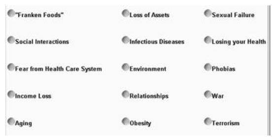
Figure 1: The 15 different studies in the Deal With It! Project

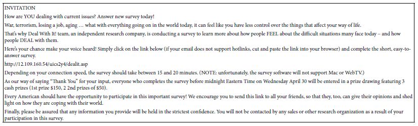
Table 1 presents a screenshot of the structure of the invitation as would be sent to the respondents. The invitation provides enough information about the study to engage respondents who are interested, but has no information about what might be an ‘appropriate answer.’ The invitation provides information about the length of time (15-20 minutes), and about the incentive (a drawing for money prizes).

Table 1: The draft version of the invitation to be sent to respondents.

The Raw Materials for the Study

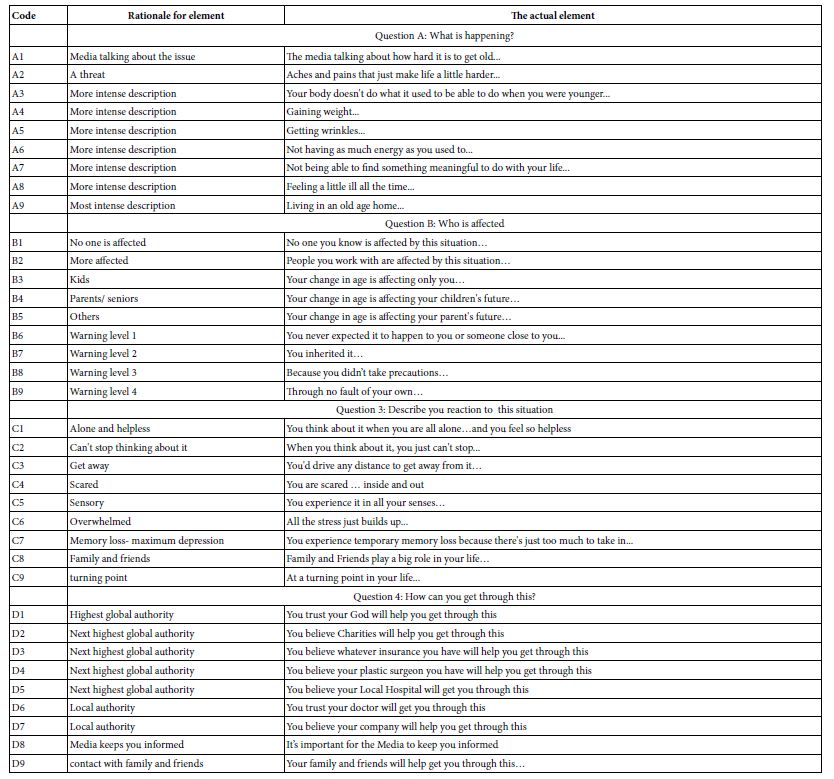
Table 2 presents the elements and the rationale for the elements. The driving force in the It! studies was to create a series of elements which represented different aspects of anxiety. Since the It! studies were to deal with 15 different topics, the elements were slightly modified by topic (e.g., aging vs obesity) in order to make ‘sense’  The elements were kept as parallel as possible across all 15 studies.  The language of the element was made as colloquial as possible while maintaining clarity. Finally, some of the elements presented the information as a description, other elements presented the information as if one were talking to oneself, or describing one’s emotions to another, but always from the point of a third person.

The 36 elements or answers in Table 2 fall by design into four groups, four questions. The purpose of the question is to drive the answer, to make sure that the answer ‘fits’ the question. In the end, however, the question itself is only a bookkeeping device, to make sure that the question does not generate answers which ‘don’t belong’. That bookkeeping property, to keep the ‘meanings’ straight, means that two or more different answers, statements which are of the same type but convey mutually contradictory information, will never appear in the same vignette.  The respondent need not see the questions. Only the response to the answers is important because that is where the relevant information lives.

Table 2: The four questions, the nine answers to each question, and the rationale for each element. The respondent never saw the rationale for the element, but only the element itself.

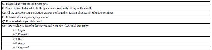
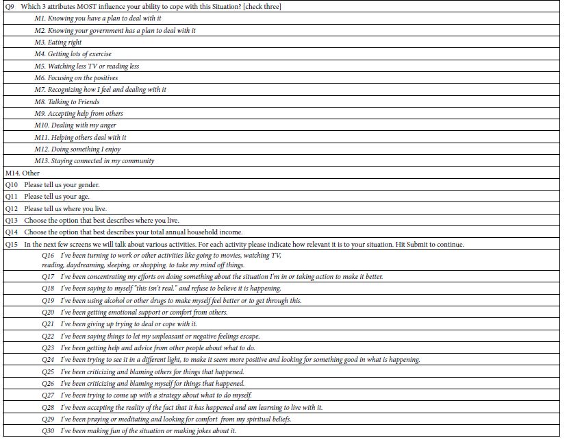
The actual interview required about 15-17 minutes. The interview was structured, beginning with the introduction to the topic shown in Table 1, followed by the presentation of 60 vignettes. The vignettes were absolutely different from one respondent to another, ensured by the ‘permutation’ of the basic experimental design. Finally, the respondent completed an extensive self-profiling  questionnaire shown in Table 3.  The self-profiling questionnaire will permit the correlation between how the respondent describes herself/him and the pattern of reactions to the elements.

Table 3: The self-profiling questionnaire

It is important to emphasize that the respondent cannot possibly ‘game’ the Mind Genomics system, simply because the elements are presented in groups of two, three, and four, respectively, in a way which seems utterly ‘random’ to most respondents. Indeed, when respondents describe their feelings about the study, doing so after the fact in follow-up contacts, many say that they feel that their answers are totally random, and they are guessing

Data Transformation at the Level of the Individual Respondent

A key benefit of Mind Genomics is the ability to create an individual-level model relating the presence/absence of the 36 elements to the ratings or to transforms of the ratings.  The responses themselves may either be the original 1-9 rating or, more typically in Mind Genomics studies, a transform of the 1-9 scale.  The transform changes ratings of 1-6 to 0, and ratings of 7-9 to 100, and afterwards adds a vanishingly small random number to each transformed number. The rationale for doing that is to prevent all 60 ratings from one respondent to be transformed into either 0 (in the case where all ratings lay between 1 and 6), or 100 in the case where all ratings lay between 7 and 9). The vanishingly small random number ensures that the transformed rating has some marginal degree of variability, allowing the OLS (ordinary least-squares) regression to work.

The scientific rationale for the conversion to a binary scale is that very few people really understand what the scale values actually mean. Thus, the typical manager will ask for clarification of the data, when all that is needed is an explanation of what the presented averages ‘really mean!. According to S.S. Stevens, the aforementioned founder of modern-day psychophysics, the hardest thing in science is to move from a continuous function to a discontinuous function, viz., to chop a continuum into meaningful components.

After the conversion is made, the data from each respondent is subject to the statistical procedure of OLS (ordinary least=squares regression), colloquially called ‘curve fitting’ [19]. The objective is to deconstruct the transformed ratings for a given respondent to the contribution of each of the 36 elements. Recall that each respondent rated 60 unique vignettes and that the 36 elements were combined in ways that ensured that the elements would be statistically ‘independent of each other. This effort pays out handsomely, allowing the regression model to describe the relation between the elements and the ratings by the equation:  Binary Rating = k₀ + k₁(A1) + k₂(A2) … k₃₆(D9).

This simple equation, estimated separately for each respondent, produces a matrix of data, one row for each respondent. Each row in the matrix comprises the additive constant, followed by 36 columns of numbers, each column corresponding to one of the 36 elements.  The coefficients tell us the estimated contribution of each element to the binary transformed rating.  One can imagine this column of data multiplied 98 times, to create 98 rows of data, one row for each of the 98 respondents who participated.

Table 4 shows the output of the regression modeling for three respondents, #1,#2 and #3, respectively. The model features an additive constant (estimated binary transformed rating in the absence of elements, a purely theoretical parameter, but a good baseline), and then 36 rows, one row per coefficient.  Table 4 is ‘transposed,’ so that the rows correspond to the 36 elements. The transposition from row to column is made simply to show the large table in an easy-to-read format.

Table 4: Example of coefficients for three respondents< #1, #2, #3, emerging from individual-level regression, and the recoding of those coefficients (0 unless coefficient is greater than 8, in which case it is transformed to 100).

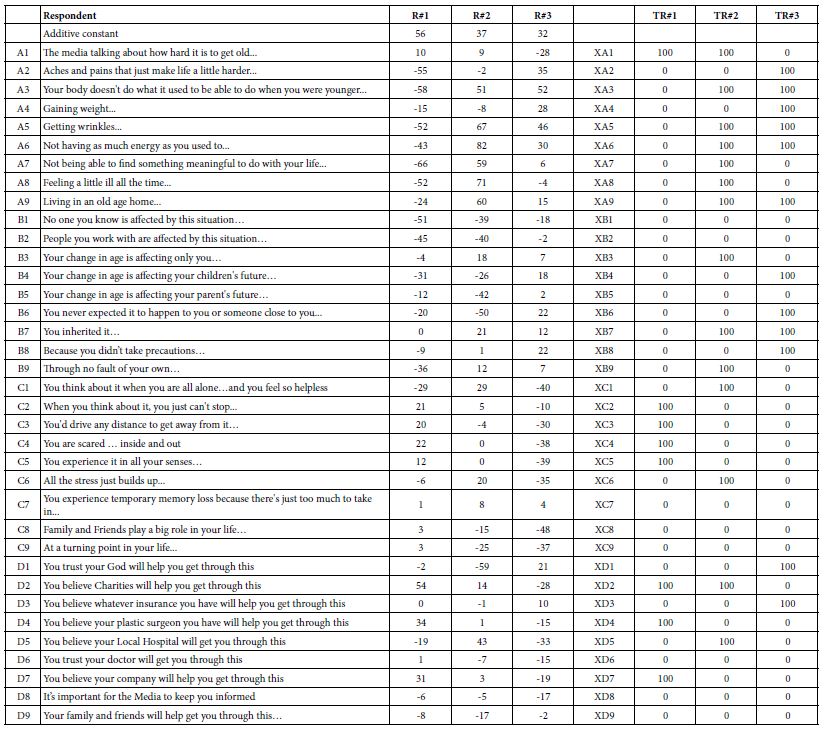
Statistical analysis of the modeling suggests that coefficients of +8 or higher are ‘statistically’ significant, viz., that they are probably not 0. In view of that, we end up learning more by ‘taming’ the wide range of coefficients. The taming consists of replacing all coefficients of 8 or higher by 100 to show that the element drives anxiety (cannot deal with it, viz., rating of 7-9). The transform further replaces all coefficients lower than 8 by 0, to show that the element does not drive anxiety (rating of 1-6 on the 9-point scale, the region where the respondent feels that the vignette does not drive the feeling of anxiety).  In Table 4 the original coefficients for respondents 1-3 are labelled R#1, R#2 and R#3. In turn the transformed coefficients for the same three respondents are shown to the right, and labelled TR#1, TR#2, and TR#3, respectively.  The elements are now renamed to be XA1, to denote that numbers associated with them are the newly transformed 0/100. The foregoing may seem to be a great deal of work, but the analysis will show the patterns far more easily.

Results

We begin with the average transformed coefficients from the total sample of 98 respondents (Table 5). For the total panel, we look at all 36 coefficients, as well as the additive constant, which was not transformed.  The additive constant is 28, meaning that in the absence of anything else except knowing the topic is ‘aging,’ 28% of the respondents would rate a vignette 7-9.  All vignettes comprised 2-4 elements by design, so the additive constant is an estimated parameter.

It is the averages of the transformed coefficients which are of major interest.  In Table 5, as well as in the other tables of averages, those elements are shaded which generate a value of 50 or higher. This cut-off means that across all 98 respondents, 50% or more generate coefficients of +8 or higher for a specific element. We would conclude that this element drives anxiety.

Table 5: The averages of the transformed coefficients for the total panel. The 36 coefficients are sorted in descending order. Averages of 50 or higher are shaded.

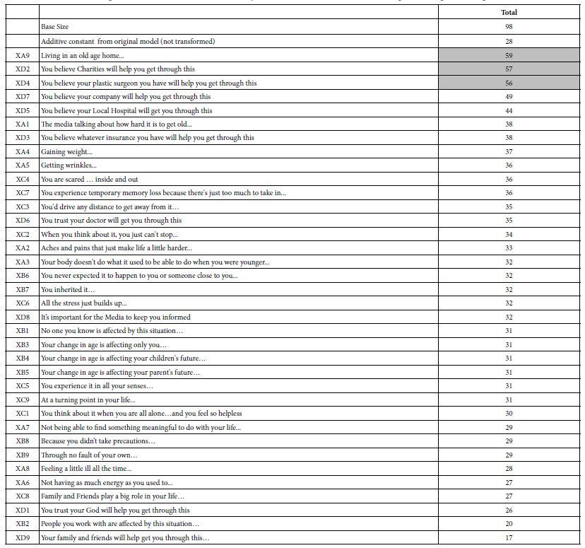
The averaging suggests three major worries:

a. Living in an old age home (viz., loss of independence)

b. You believe Charities will help you get through this (viz., loss of economic independence)

c. You believe your plastic surgeon you have will help you get through this (loss of attractiveness and vitality).

Table 5 suggests that there are some common, but not necessarily universal fears about aging. What is remarkable is that these fears ‘make sense’ and are easy to interpret, even though as noted above, the vignettes seem to be, in the words of Harvard psychologist William James, a ‘blooming, buzzing confusion’, leaving respondents feeling that they were just guessing when their data seems quite reasonable, at least in terms of the average.

Creating Easier to Read Tables of Data

Mind Genomics studies generate large tables of data, especially when the elements are ‘cognitively meaningful’ in and of themselves, rather than being points which make sense only in patterns. With Mind Genomics the individual elements carry with the richness of experience and an invitation to reflection and explanation.

The early Mind Genomics studies, of which this study is an example, comprise four questions, nine answers, and thus 36 elements. Thus, each subgroup to be considered generates 36 averages. That amount of data overwhelms, becoming a ‘wall of numbers.’  The way out of the quandary is to eliminate all data with averages less than 50 and to eliminate all elements which fail to generate an average of 50 for at least one subgroup. This first step, pruning, shortens the data tables, making the patterns easier to discern.

The second step ranks the elements and ranks the subgroups, both in descending order, so that the top element is the one with the strongest performance across the different subgroups (called Row Sum), and the strongest subgroup (is the one with the strongest performance across the different elements (called Column Sum). These two statistics, row sum and column sum allow the strong performing elements to emerge. The pattern is easy to identify since the only data in the table are averages of 50 or higher.

Differences by ‘Time of Day’?

The first question in the self-profiling questionnaire was the time of day in two hour sections. Although we don’t typically think of studies as influenced by when the respondent participated, part of the issue with the Deal With It! series was to search for deep, hitherto unexplored effects.  Following the approach described above, Table 6 shows the strong performing elements by time of day.

Table 6: Average transformed coefficients by ‘time of day’. On strong performing averages of 50 or higher across the appropriate respondents appear in the table.

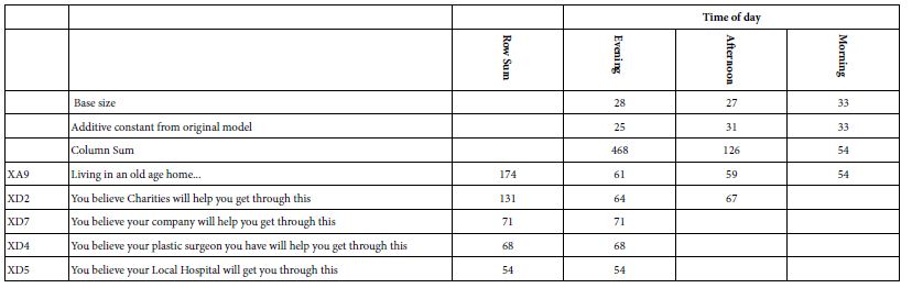
The first thing to notice about the data in Table 6 is that there are only five elements. One element is ‘living in an old age home…’, which will reappear in analysis after analysis. The other four strong performing elements are the response to statements that others (e.g., Charities) ‘will help you get through this.’ Clearly, relying on a second party outside of one’s control causes anxiety, even though the statement is meant to be a statement that there is someone else to help.

The second thing to notice is that the respondents who participate in the evening show far greater anxiety, whereas the respondents who participate in the afternoon and the morning show far less anxiety. We see that from the column sums of strong performing coefficients (468 for evening, 126 for afternoon, and only 54 for morning.

Finally, the additive constant from the original, untransformed model, average around 25-33, suggesting a low predisposition for an anxious response. Recall that the additive constant is an estimated parameter that shows the percent of responses 7-9 to be expected in the absence of elements. In other words, the additive constant is an estimated baseline.

Differences by WHO the Person is (Gender, Age, Income, Where the Person Lives)

The extended self-profiling classification shown in Table 3 allows us to learn a lot about who the respondent is.  The questions, ranging from gender to age, income, and even neighborhood, may produce some new insights into what concerns the respondent. With that in mind, we now look at Tables 7-10.

Gender (Table 7): The respondents comprised primarily females, a distribution which often is corrected for by oversampling males until a balance is reached. In the It! studies, starting back in 2001 and continuing until 2004 for all of the It! studies, no effort was made to balance the genders. With 15 studies in the Deal With It! project, and with a limited budget, gender balancing might be laudable but unaffordable.

Table 7 shows the strong performing elements. Both males and females begin with modest basic anxiety (additive constant 31 vs 28, based on the original model, before transformation).  It is when we get to the performance of the specific elements that we see the dramatic gender differences.  The one element which makes both males and females very nervous is XA9, living in an old age home, with the value for the males 83, and the values for the females 56. We interpret that to mean that 83% of the males feel that living in an old age home is something with which they could not deal. Females were less responsive, with a coefficient of 45, meaning 56% of the females respond that they could not deal with it. Keep in mind once again that the respondents were not directly asked about living in an old age home, but rather than element was part of a set of 2-4 elements combined into a vignette.

Table 7: Average transformed coefficients by ‘gender’. On strong performing averages of 50 or higher across the appropriate respondents appear in the table.

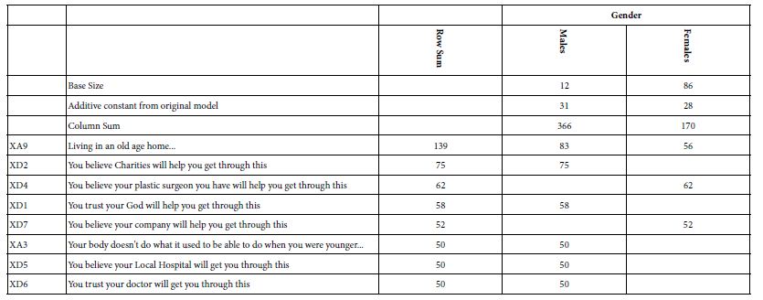
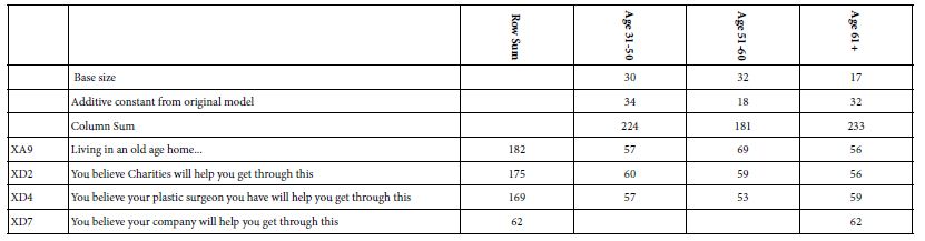
Table 8 shows the strong performing elements by age.  The columns are arranged by age, rather than by column sum to allow any age-related pattern to emerge.  Once again we see the same three elements emerging as most anxiety provoking (living in an old age hold, help from charities, help by plastic surgeon) The one major new entry, not surprisingly, is the response from the older respondents (age 61+) who are most frightened when they read ‘You believe your company will help you get through this.’ Their strong response to this element, even twenty years in 2003, suggests that older people near or past retirement are insecure and nervous when they think of their companies as providing any help to older employees or former employees.

Table 8: Average transformed coefficients by ‘age’. On strong performing averages of 50 or higher across the appropriate respondents appear in the table.

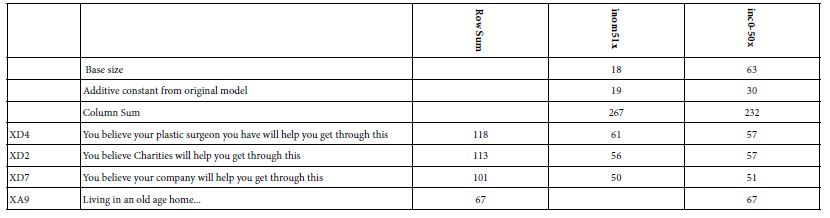
Income tells the same story as age, as shown in Table 9.

Table 9: Average transformed coefficients by ‘income’. On strong performing averages of 50 or higher across the appropriate respondents appear in the table.

Respondents selected the type of neighborhood in which they lived. Table 10 shows that there is a great disparity in the distribution of the strong responses by neighborhood. Those respondents identifying themselves as living in a city, but a suburban (residential) area in the city showed the greatest number of elements which drove anxiety.

Table 10: Average transformed coefficients by ‘type of neighborhood in which the respondent resides’. Only strong performing averages of 50 or higher across the appropriate respondents appear in the table.

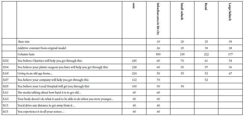
When we look at the data more deeply, however, we find that the strong performance is due to a few anomalies. These elements drive anxiety for only one or two groups of respondents

1. You believe your company will help you get through this -Suburban area, Rural
2. You believe your Local Hospital will get you through this – Suburban area, Small suburb
3. The media talking about how hard it is to get old… – Suburban area
4. Your body doesn’t do what it used to be able to do when you were younger… – Suburban area
5. You’d drive any distance to get away from it… Suburban area
6. You experience it in all your senses… Suburban area

If we discount these six elements are relevant to one subgroup, or at most two, we end up with the same elements which are responsible for the strongest anxiety, namely charities, plastic surgeon, and old age home.

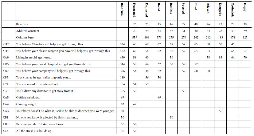
Is There a Relation between What a Respondent ‘Feels’ and the Pattern of Elements Which Drive Anxiety?

Question 6 of the self-profiling questionnaire asked the respondent to introspect about how she or he feels and check all the emotions on a list which apply.  The question did not attempt to link the feelings to the vignettes because the respondent had just evaluated 60 vignettes. Nonetheless, it is instructive to look at the covariation between what a respondent selects as anxiety product (rating 7-9) and what feelings the study leaves with the respondents.

Table 11 shows the table, once again in the standard format. The dynamics of the data remain generally the same. That is, there are the three major aspects driving anxiety (charities, plastic surgeon and old age home, respectively). These generate the highest sum for the three most negative feelings (frustrated, depressed, bored). The other two elements which co-vary most strongly with these emotions deal with the local hospital and one’s own company. Based upon the data from the previous analyses, these strong performing elements do not surprise. Four of the elements deal with being helped, when one needs help (charities, plastic surgeon, hospital, one’s own company). There is once again a sense of being frightened that these presumed ‘allies in life’ will prove actually impotent, or unwilling to help. The fifth one, old age home, speaks to a sense of helplessness.

The right side of Table 11 shows the selected emotions with the lowest column sums, viz., the lowest degree of causing anxiety across the 36 elements. These four emotions/feelings, from the lowest up, happy, optimistic, energetic, and relaxed, four positive emotions. The elements which drive anxiety for people reporting these emotions are the ones that we have to come to expect, namely charities, plastic surgeon and old age home.

Table 11: Average transformed coefficients by selection of up to three emotions experienced by the respondent after having evaluated 60 vignettes. Only strong performing averages of 50 or higher across the appropriate respondents appear in the table.

The ability to cross-reference one’s selected emotions at a given time with the elements driving anxiety creates a new opportunity for Mind Genomics. There is now the possibility of looking at the covariation of emotions and anxiety producers, in a situation where the respondent cannot possibly ‘game’ the system.

Deconstructing the Respondents into Mind-sets Based Upon the Pattern of the Coefficients

A hallmark of Mind Genomics is the ability to cluster the respondents into different groups, so-called mind-sets, based upon the pattern of coefficients. Clustering is a well-defined class of statistical processes which divide a group of objects (e.g., people) into non-overlapping groups, based upon the pattern of measures [20]. For our study clustering is done by dividing our 98 respondents into two and then into three groups, clusters, viz., mind-sets, based upon the pattern of their 36 coefficients.

The regression analysis already provides us with the additive constant and the 36 coefficients for each of our 98 respondents. This within-subjects modeling is feasible because each respondent evaluate the precise combinations needed to create a linear regression equation relating the presence/absence of the 36 elements to the binary transformed response.  The 36 estimated coefficients from the individual-level OLS (ordinary least squares) become the 36 variables on which the k-means clustering is done. The analysis created two and then three clusters, or mind-sets, creating them by assigning each of the 98 respondents to one of the three non-overlapping cluster.

Table 12 shows the results for the two and three mind-sets. To maintain consistency, the mind-sets were created using the estimated coefficients emerging from regression. Afterwards, the coefficients were once again transformed, so that coefficients of 8 or higher were transformed to 100, coefficients below 8 were transformed to 0. In short, the clustering into mind-sets produces new subgroups, not based on who they say they are or what they feel, but rather based on how they respond to the different statements. The power of clustering is that it puts together people with similar points of view, and in effect gets rid of the extraneous material which may seem relevant but is not. As a consequence, the mind-sets are a great deal more focused with almost no extraneous elements.

Table 12: Average transformed coefficients by two and three emergent mind-sets resulting from k-means clustering. Only strong performing averages of 50 or higher across the appropriate respondents appear in the table.

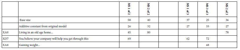
Based upon the strong performing elements we may offer these names to the mid-sets (MS)>

Two mind-sets:

MS 1 of 2 – Betrayal – Worry about being let down by one’s own company

MS 2 of 2 – Loss of freedom – Worry about living in an old age home

Three mind-sets:

MS 1 of 3 –  Betrayal – Worry about being let down by one’s own company

MS 2 of 3 –  Betrayal and Beauty – Worry about being let down by one’s own company AND gaining weight

MS 3 of 3 – Loss of freedom – Worry about living in an old age home

Discussion and Conclusion

The use of a combination of elements (vignettes) and the use of different combinations (‘permutations)’ scheme deserve their own notes because of the contribution that they make to science. In attitude and consumer research quite often the respondent is biased, either with awareness (viz., getting it right) or without awareness. Researchers have been aware of the biases involved when respondents feel that there is an expectation for them to be consistent, or for them to give the right answer, for whatever reason.  Allowing the respondent to answer questions one by one gives the respondent a chance to reframe the criterion each time, to be appropriate to the question. The typical researcher may not even realize that the respondent is reframing, changing the criterion, given the right answer for some questions, and the true answer to others. One need only work with dietitians who, upon working with the client for the first and doing the ‘intake’ find the client to report being a model citizen with no ‘bad stuff’ in the house. That is the ‘correct’ answer, which should make the dietitian happy. Inspection of the house will reveal lots of foods which are never reported, overlooked.  The use of vignettes prevents some of this changing criterion to always give the right answer. To once again quote the words of Harvard psychologist Wm James, the vignettes present a ‘blooming, buzzing confusion’ to the respondent. It is simply impossible with these 2-4 element vignettes to know what is the ‘right answer’. Most respondents end up guessing, or feel that they are guessing. Yet their data suggest just the opposite, viz., that they are consistent, but relaxed, maybe even bored.

The second topic is the permutation. Typically, science works by choosing a promising area, testing in that area, and reducing the error of measurement by making many measurements of the same area. The ingoing but unspoken assumption is that this area is the ‘correct’ area, such assumption rarely eally questioned in terms of its validity because the effort to replicate is too difficult, expensive, and of course discouraging. In the meanwhile, no matter how the area is discovered, usually by prior knowledge and good guesswork, the researcher ends up shoring up the measurement of perhaps a wrong area by reducing the error of measurement. The reduction, not so much by exploring other possible areas in the ‘space,’ but rather piling on more respondents to test the same vignettes. The goal is to get a better measurement, a more precise measurement, but of course with the scarcely acknowledged possibility that the whole enterprise is looking into the ‘wrong’ area. This is the hypothetico-deductive method research [21].

Mind Genomics lies outside the standard realm of hypothetico-deductive research. One can think of Mind Genomics as a mapping exercise, a cartography, to discover information about how we think. One could use the method for hypothesis, but the research strategy is simply to create ideas about a topic, mix them, get reactions and determine how the ideas drive the reaction. There may be theory, or simply a mapping exercise. Like an explorer, one can study areas in which one is an expert or conversely areas in which one is completely ignorant. The data are accretive, as more and more of the topic area is explored by study after study. The end result is a database of the mind, created in what ends up being an efficient inexpensive, possibly results-directed manner or possibly random exploration, all at a lower price.  In other words, the world view of Mind Genomics is to increase knowledge, and create a small or a large database about a specific topic.  The topic may be virtually anything to which a person can respond after reading a description, as long as an underlying experimental design can create alternatives to the basic idea.

The third topic is simple. What did we find?  It’s about old age homes, ineffective plastic surgery, and financial ‘betrayal.’

Acknowledgment

The author acknowledges the original efforts to collect the data though It! Ventures LLC, and is especially grateful to the late Hollis Ashman for her efforts at putting together the study, and doing the preliminary analyses in 2003, when the data were first collected.

References

1. Barrett AE, Robbins C (2008) The multiple sources of women’s aging anxiety and their relationship with psychological distress. Journal of Aging and Health 20: 32-65. [crossref]
2. Ramírez L, Palacios-Espinosa X (2016) Stereotypes about old age, social support, aging anxiety and evaluations of one’s own health. Journal of Social Issues 72: 47-68.
3. Richardson TM, Simning A, He H, Conwell Y (2011) Anxiety and its correlates among older adults accessing aging services. International Journal of Geriatric Psychiatry 26: 31-38. [crossref]
4. Lynch SM (2000) Measurement and prediction of aging anxiety. Research on Aging 22: 533-558.
5. Lasher KP, Faulkender PJ (1993) Measurement of aging anxiety: Development of the anxiety about aging scale. The International Journal of Aging and Human Development 37: 247-259. [crossref]
6. Noh JH, Lim EJ (2014) Factors influencing Rural Elderly Women’ Health Promotion Behavior. Advanced Science and Technology Letters 61: 44-47.
7. Mehta KM, Simonsick EM, Penninx BW, Schulz R, Rubin SM, et al. (2003) Prevalence and correlates of anxiety symptoms in well-functioning older adults: Findings from the health aging and body composition study. Journal of the American Geriatrics Society 51: 499-504.
8. Stevens SS (1966) Personal communication to Howard Moskowitz
9. Green PE, Krieger AM, Wind Y (2004) Thirty years of conjoint analysis: Reflections and prospects. In Marketing research and modeling: Progress and prospects, 117-139, Springer, Boston, MA.
10. Anderson NH (2014) Contributions to Information Integration Theory. Volume 1. Cognition. Imprint Psychology Press.
11. Mead R (1990) The design of experiments: statistical principles for practical applications. Cambridge University Press.
12. Moskowitz HR (2012) ‘Mind genomics’: The experimental, inductive science of the ordinary, and its application to aspects of food and feeding. Physiology & behavior 107: 606-613. [crossref]
13. Moskowitz HR, Gofman A, Beckley J, Ashman H (2006) Founding a new science: Mind genomics. Journal of sensory studies 21: 266-307.
14. Moskowitz HR, Wren J, Papajorgji P (2020) Mind Genomics and the Law. Lambert Academic Publishers, Germany.
15. Gabay G, Moskowitz H, Onufrey S, Rappaport S (2017) Predictive modelling and mind-set segments underlying health plans. In Applying predictive analytics within the service sector, 135-156. IGI Global.
16. Gofman A, Moskowitz H (2010) Isomorphic permuted experimental designs and their application in conjoint analysis. Journal of Sensory Studies 25: 127-145.
17. Rabino S, Moskowitz H, Katz R, Maier A, Paulus K, et al. (2007) Creating databases from cross-national comparisons of food mind-sets. Journal of Sensory Studies 22: 550-586.
18. Moskowitz HR, Beckley J, Ashman H (2009) Beyond anxiety and political correctness’: How experimental design trumps’ gaming it’ and gets more deeply into the mind. Available at SSRN 1438648.
19. Craven BD, Islam SM (2011) Ordinary least-squares regression. The SAGE Dictionary of Quantitative Management Research 224-228.
20. Likas A, Vlassis N, Verbeek JJ (2003) The global k-means clustering algorithm. Pattern Recognition 36: 451-461.
21. Kell DB, Oliver SG (2004) Here is the evidence, now what is the hypothesis? The complementary roles of inductive and hypothesis-driven science in the post-genomic era. Bioessays 26: 99-105.

DOI: 10.31038/ASMHS.2022653

Abstract

The paper presents a new approach to optimizing the shopper experience, combining easy-to-implement tools for understanding shopper mind-sets at the granular, specific level (Mind Genomics; www.BimiLeap.com) with a simple, rapid way which assigns any shopper or prospective shopper to the relevant mind-set for that granular topic (www.PVI360.com). The approach begins with a simple study of the motivating power of relevant messages and thus uncovers mind-sets or groups of respondents showing similar patterns of what motivates them. Then, using the same data, the approach creates a simple questionnaire comprising six questions taken from the original study, the pattern of answers to which assigns a new person to a mind-set. Once the mind-set of the shopper is ‘identified’ for the granular topic using the PVI (personal viewpoint identifier) it is a matter of giving the shopper the appropriate motivating message, either at the time of shopping in brick and mortar store or e-store, or sending the message on the Internet in the form of an advertisement or individualized coupon.

Introduction

The past two decades have seen an explosion of knowledge about the consumer, the knowledge emerging from the speed and affordability of internet-based surveys, the sophisticated analysis of masses of cross-sectional data known as Big Data, and the application of artificial intelligence to uncover patterns. What continues to emerge is that nature is simultaneously tractable and intractable. As the macro level we know what to expect in terms of purchase patterns and expected time to repurchase, some of which knowledge may transfer to the level of the individuals, only for the general pattern just exposed to be disrupted by the idiosyncrasies of each individual.

The world at the time of this writing (Fall, 2022) is quite different from the world of just a decade ago, and most certain far different from the earlier decades. The notion that one could change advertisements is well-accepted, easily and widely done. Outdoor advertisements and LED technology assault us everywhere we go. We are accustomed to see large billboards with attention-grabbing sequences advertisements, the modern day evolution of signage of decades ago, once static, now plastic, and changeable at will. Now technology makes it possible to individualize the messaging for an individual, much as is done on a cell phone. This paper presents one approach.

The organizing nature of this paper is how one might advertise to a single customer, using science to uncover the ‘mind’ of that customer ahead of time. The objective of this study was to understand the different types of messages which might appeal to shoppers of cereal in the middle isle, and shoppers of yogurt in the refrigerated dairy section. Could the technology of 2022 be set up to deliver the proper messages to an individual who is walking along the store? And could the approach be set up to be done at scale, affordably, quickly, with scientific precision rather than with guessing about what the person wants based upon who the person is. This latter condition is important. It means that the messages must be delivered to the person most likely to respond to the specific messages.

The studies reported here were done with the intention of testing out the possibility that one could create a knowledge-based system about messaging for simple, conventional, familiar products. The paper does not deal with new to the world products which have their own mystique, and both positive and negative messaging attached. Rather, the paper deals with what one might call ‘tired, old, utterly familiar’ products that may not be susceptible to the romance of the new and different.

A Short Historical Overview to ‘Messaging the Shopper’

The notion that one can influence the shopper by proper messaging is decades old, and the subject of numerous experiments. Indeed, the real-world behaviors of shoppers and the change in behavior resulting from the proper messaging opens up the topic to anyone interested in messaging, whether the interest be theory such as experimental psychology, to applied science such as consumer psychology, and of course the world of business applications. As a consequence, there have been a number of different studies focusing specifically on shopping.

1. Schumann et al. [1] reported only modest effectiveness of signage in shopping cart. To summarize their results: “Findings from both studies reflect that over 60% of the 2 samples noted the presence of the signs in their carts. When Ss were questioned about their awareness of cart advertising on a specific occasion, only 3.0–6.5% recalled the product. There was no evidence that cart signage acts in a subliminal fashion that results in the purchase of the brand.” It may well be the signage in the cart was general information about the product, not necessarily information that would tug at the heartstrings of the shopper.
2. Dennis et al. [2] confirmed the efficacy of digital signage but argued for emotional content. They noted that the typical content of digital signal is ‘information-based’ whereas digital signage might be more effective if it were to comprise emotional messaging as well, or even instead of simple information. Results are limited as the DS (digital signage) screens content was information based, whereas according to LCM, (Limited Capacity Model of Mediate Messaging) people pay more attention to emotion-eliciting communications. The results have practical implications as DS appeals to active shoppers.
3. Buttner [3] proposed at two types of shopping orientations (mind-sets), task focused and experiential shopping, respectively. They report that “Activating a mindset that matches the shopping orientation increases the monetary value that consumers assign to a product. …. marketers and retailers will benefit from addressing experiential and task-focused shoppers via the mindsets that underlie their shopping orientation.”
4. Chang et al. [4] reported that mind-sets are important, and that the communication should consider the different mind-sets. Their notion was that people may or may not be skeptical to advertising. Those who have a ‘utilitarian orientation’ and an ‘individualistic’ mind-set tend to be skeptical about advertising, and need messages which are different from those individuals who have a ‘hedonic’ and a ‘collectivistic’ mind-set. Chang and Chen bring this topic into discussions about CRM and donating, but their notions can be easily extended to the right type of messaging for digital signage.

The Contribution of Mind Genomics to the Solution

Mind Genomics is an emerging science which grew out of the need to understand how people make decisions about the issues of the ‘everyday’. Mind Genomics rests on the realization that the ‘everyday’ situations are compounds of different stimuli. To study these stimuli requires that the respondent, the test subject, be confronted by compound test stimuli which comprise different aspects of everyday situation, stimuli that the respondent ‘evaluates’, such as rating the combination. Through statistics, applied after the researcher properly sets up the blends, it becomes possible to understand just exactly what features ‘drive’ the rating. Properly executed, this seeming ‘roundabout way’, testing mixtures, ends up dramatically revealing the underlying mind of the respondent [5,6].

The foregoing process, testing systematically created mixtures and deconstructing through statistics, stands in striking opposition to the now-hallowed approach of ‘isolate and study.’ The traditional approach requires that the features of the everyday be identified, and separately evaluated, one feature at a time. Typically the evaluation ends up presenting each of the features separately, getting a rating, analyzing the pattern of ratings across people, and then identifying the key variables which a difference.

Attractive as the traditional methods may be, the one-at-a-time is severely flawed for several reasons:

1. Combinations of features are more natural. It may be that a feature will receive a different score when evaluated alone compared to the evaluation of the feature as part of a mixture. And it may be that the feature will receive different scores when evaluated against backgrounds provided by a variety of other features. Thus, the wrong answer may emerge.
2. People may change their criterion of judgment when presented with an array of different types of features, such as features dealing with product safety versus features dealing with branding, with benefits, and so forth. All too often the researcher AND the respondent fail to recognize the underlying shifts in these criteria.
3. It becomes very difficult to ‘game the system’ when the test stimulus comprise a combination. Often, and perhaps even without knowing it, the respondent tries to assign the ‘correct’ or ‘socially appropriate’ answer. Such effort to ‘be right’ is doomed to failure when the respondent is presented with a combination. Often the respondent asks the researcher or interviewer for ‘help’, such as asking ‘what do I pay attention to in this combination?’

Mind Genomics works with the response to combination of text messages, called vignettes. The vignettes comprise specified combinations of elements, viz., verbal messages. Table 1 below (left part of table) shows these messages. The messages are sparse, to the point, paint a word picture. The vignettes are created according to an underlying plan called an experimental design. The experimental design may be thought of as a set of different combinations, different recipes, combining the same messages, the same elements, in different ways.

Table 1: Positive elements for cereal, viz., and those elements which drive the rating of a vignette towards definitely buy/probably buy). All elements shown have positive coefficients of +2 or higher.

A key difference between Mind Genomics and conventional research is how Mind Genomics considers variability among people and how it deals with that variability. We start the comparison by considering conventional research, which often considers variability in the data to be error, usually unwanted error which masks the ‘signal’. Occasionally the variability can be traced to some clear factor, such as the nature of the respondent, in which case this irritating variation hiding the signal is actually a signal itself. For the most part, however, researchers consider variability to be unwanted, and either suppress it by meticulous control of the test stimulus/situation, or average out the variability by working with a lot of respondents, and assuming that the variability is random, and so will cancel out.

In the world of Mind Genomics variability is considered in a different light. Certainly there is the appreciation of error, but there is also the acceptance of the fact that people differ from each, and that these differences may be important. The differences between people are not necessarily random error, but rather point to potential profound differences among people, albeit differences which exist in a small, granular aspect of daily life. In other words, sometimes the differences are important, and sometimes the differences are merely random noise.

Explicating the Research Process

For the project reported here, the researcher selected two products (cereal, yogurt), asked six questions about the product, questions that could be used to create consumer-relevant messages, and then developed the database of 36 possible consumer messages for each product.

Thus far, the process is quite simple; requiring only that the researcher do a bit of thinking about what types of messages might be relevant to consumers. One of the in-going ‘constraints’ from the perspective of marketing and the trade was that the messages had to be of the type which drive purchase. It was not an issue of building one’s brand through advertising. Rather, the messages were chosen so that they could be put on a coupon, or flashed on an LCD panel as the respondent ‘walked by.’

The actual process of developing the raw materials can be daunting for those who are not professionals. In the two studies reported here, a significant effort was expended to develop the six ideas which tell a ‘product story’. One the six ideas are developed, the most intellectually intense part of the effort, the creation of six messages for each idea becomes much easier. Recently, the creation of these basic ideas (or questions), and the elements (or answers) has been improved by a process called Idea Coach, which provides different options, using artificial intelligence (www.BimiLeap.com). The data reported here were collected before the Idea Coach system was incorporated into Mind Genomics:

1. The actual selection of messages generated six groups of six message, one set of 36 such messages for cereal (Table 1), and another set of comprising different messages, for yogurt (Table 2).When looking at the table, the reader should keep in mind that the elements either pain a simple word picture, or specify a specific a specific claim that could be turned into ‘copy.’
2. When creating the messages and assigning them to groups, the only requirement for the researcher is to ensure that all of the messages in a single idea (viz., all the answers given to a single question) remain together. For example, messages about ‘calories’ must all be put into one group or idea, and not split across two groups or questions. The rationale for this requirement comes from the fact that the underlying experimental design will need to combine elements from different questions (described below). When the researcher puts a calorie message in one group, and another calorie messages in a second group, there is the likelihood that the underlying experimental design may put these mutually incompatible messages into the same combination.
3. Once the elements are created, comprising the question and the six answers, as shown in Tables 1 and 2, the next step is to use the basic experimental design, which specifies 48 combinations, each combination comprising either three or four elements. Each combination or vignette contains at most one element from any question. The vignettes are by design incomplete, since there are six questions, but a vignette can only have three or four answers, one from three or four questions. As noted above, each respondent evaluates a unique set of 48 combinations. The underlying mathematics remains the same. What changes is the assignment of a message to a code. For example, for one person, element A1 may be assigned as A1, whereas for another person a permutation is done, so the former A1 becomes A2, A2 becomes A3, et. the experimental design is maintained, but the combinations change [7].
4. The final steps comprise the introductory message and the rating scale. In Mind Genomics studies most of the judgment must be driven by the individual elements, and not by the introductory statement. It is better to be vague about the product, and let the individual elements drive the reaction, rather than to specify too much in the general introduction. For this study, the introduction was simply ‘Please read this description of cereal and rate it on the 5-point scale below. For yogurt the introductory statement was virtually the same ‘please read this description of yogurt and rate it on the 5-point scale below’
5. The five-point rating of purchase is anchored: 1=definitely not buy, 2 = probably not buy, might not/might buy, 4= probably buy, 5 = definitely buy. The anchored five point purchase intent scale has been used for many decades in the world of consumer research, both because the scale is sensitive to differences and because managers understand the scale, and generally look at the percentage of responses that are 4 and 5 on the 5-point scale. These two rating scale points are probably buy and definitely buy. The scale is often transformed to a binary scale, as was done here. Ratings of 4 and 5 were transformed to 100. Ratings of 1, 2 and 3 were transformed to 0. Managers who use the data more easily understand a yes/no scale, buy/not buy.
6. Following the evaluation of 48 vignettes, the respondent completed a short self-profiling questionnaire, providing information about gender and age.
7. Respondents were sent one of two links, the first appropriate to the cereal study, the second appropriate to yogurt. Approximately 70% of the individuals who were invited ended up participating. The high completion rate can be traced to the professionalism of the on-line research ‘supplier’. As a general point of view, it is almost always better to work with companies specializing in on-line research. Trying to recruit the respondents oneself ends up with a completion rate much low, often lower than 15%.

Table 2: Strong performing elements for cereal, for divisions of respondents into two complementary mind-sets, and then into four complementary mind-sets. All elements shown have positive coefficients of +10 or higher.

Creating the Database and Analyzing the Data for a Study

Each respondent ended up evaluating 48 different combinations, called vignettes, assigning each vignette a rating on an anchored 5-point scale. The next step creates a ‘model’ or equation showing how each of the 36 elements about the product ‘drives’ purchase intent. Recall that all 48 vignettes of a respondent differed from respondent to respondent, although the mathematical structure was the same. This ‘permutation’ strategy allows the research to cover a large percent of the possible combinations [7].

In order to uncover the impact of the elements, the key variables, it is necessary to create an equation relating the presence/absence of the 36 text elements about the product to the rating. This can be easily done. The data are easily analyzed, first by OLS (ordinary least-squares regression) and then by clustering. OLS regression shows how the 36 elements ‘drive’ the response (purchase). Clustering identifies groups of respondents with similar patterns of coefficients groups that we will call ‘mind-sets.’

1. The OLS regression, applied to either the individual data, or to group data, is expressed by the following: Positive Intent to Purchase = k₀ + k₁(A1) + k₂(A2) . k₃₆ (F6).
2. For regression analysis to work, the dependent variable, the transformed variable (either 0 or 100) must show some small variation across the different 48 ratings for each individual respondent. Often, respondents confine their ratings to one part of the scale (e.g. 1-2; 4-5, etc.). To avoid a ‘crash’ of the OLS regression program, and yet not affect the results in a material way, it is a good idea to add a vanishingly small random number (e.g. around 10^-4) to every transformed rating. The random number ensures variation in what will be the dependent variable, but does not affect the magnitude of the coefficients which emerge from the OLS regression.
3. The underlying experimental design for each individual respondent makes it straightforward to quickly estimate the equation, either for individuals or for groups. The coefficient, whether for individual or for group, shows the degree to the element drives the response the rating of ‘definitely or probably purchase.’ The individual coefficients, viz., for the hundreds of respondents, are typically ‘noisy’, but when the coefficients become stable and reproducible when the corresponding coefficients are averaged across dozens of respondents, or when the equation is estimated from the raw data of dozens of respondents.
4. The additive constant (k₀) shows the estimated proportion of responses that will be 4 or 5 (viz., definitely purchase or probably purchase), in the absence of elements. Of course the underlying experimental design dictated that all 48 vignettes evaluated by any respondent would comprise a maximum of four elements (at most one element from a group) and a minimum of three elements (again, at most one element from a group, not more).
5. The 36 individual coefficients (A1-F6) represent the contribution of each element to the expected interest in purchasing. When an element is inserted into a vignette, we can estimate its likely contribution by adding together the additive constant and the coefficient for the element. The sum is the percent of the respondents who would assign a rating of 4 or 5 to that newly constructed vignette.
6. One of the ingoing tenets of Mind Genomics is that there exist groups in the population which think about the same topic, but in different ways. The information to which these respondents react may be the same but these groups use the information in different ways. Some respondents may value the information so that the information appears to covary with their rating of purchase the product. In contrast, other respondents may completely ignore the information. These differences reflect what Mind Genomics calls ‘mind-sets’, viz groups of individuals with clearly defined and different ways of processing the same information.
7. The mind-sets emerge through the well-accepted statistical analysis called clustering [8]. Briefly, the clustering algorithm computes the Pearson correlation between pairs of respondents, based upon their 36 pairs of corresponding coefficients. Respondents with similar patterns (high positive correlation) are assigned to the same mind-set. Respondents with dissimilar patterns (negative or low positive correlations) are assigned to different mind-sets.
8. For this study the ideal number of mind-sets is as few as possible. The paper reports the results emerging from dividing the respondents into two mind-sets, and then into four mind-sets, to show the effect of making the clustering more granular. The focus will be on interpreting the results from the two mind-set solution, and creating a tool to assign a new person to the one of the two mind-sets.

Applying the Learning – Cereal

Our data with 328 respondents provides us a wealth of information about to say, what not to say, and to whom. Table 1 shows the results for cereal. The table is organized with the key subgroups of respondents across the top and the messages down the side. In order to make the table easier to read, and allow the patterns to emerge, the table only shows positive coefficients of 2 or higher. The other coefficients were estimated, but are not relevant to the presentation since they do not drive positive interest in purchase. Furthermore, Table 1 shows strong performing elements as shaded cells. Strong performing is defined as a coefficient of +10 or higher. Table 1 is rich in detail. The table shows the results from running the aforementioned linear equation using the data from all respondents (total), then the data by gender, then by age.

1. The additive constants differ, neither by gender nor age. Again and again Mind Genomics studies reveal that for the most part, conventional methods dividing people fail to show dramatic differences in how these divisions generate groups which think differently. It is eternally tempting to divide people by who they are, and presume that because people are different they think differently.
2. The total panel of 328 respondents shows very few positive elements, and no strong elements. That is, knowing nothing else we cannot find elements which strongly drive purchase intent. Most of the elements are blank, meaning that the coefficients for those elements are either around zero or negative. In effect, ‘doing the experiment,’ viz. evaluating different messages, fails to uncover strong performing elements. No matter what experts might think, there are no apparent ‘magic bullets’ for cereal.
3. A first effort to divide groups looks at gender. The additive constant is the same, but the females have a few more positive than do the males. Yet, none of the elements are strong drivers purchase when evaluated in the body of a vignette.
4. The second effort divides the respondents by age. In terms of the additive constant, the younger respondents (ages 18-39) show a slightly higher additive constant than do the older respondents (age 40+; constants of 58 vs 53). The only strong performer (coefficient >1= 10) is S4 for the younger respondents: The same great taste of cereal only better.
5. The third effort divides the full set of respondents into exactly two mind-set and then into exactly four mind-sets using k-means clustering [8]. To save space and make it easier for patterns to emerge, Table 2 shows the only those elements which perform strongly in at least one mind-set of the six created (two mind-sets + four mind-sets = six mind-sets). ‘Performing strongly’ is again operationally defined as a coefficient of +10 or higher. The groups with fewer strong performing elements will be harder to reach.
6. Focusing just on the two mind-set solution, Mind-Set 2 is more primed than Mind-Set to be interested in buying the cereal (additive constant of 68 for Mind-Set 2, additive constant of 38 for Mind-Set 1). However, Mind-Set 1 shows two elements which excite its members:

O2: A tasty breakfast choice makes it easy to maintain a healthy body weight

O4: Ideal choice for those concerned about eating too much sugar

Applying the Learning – Yogurt

Our second study, this time with 307 respondents, shows similar patterns. Table 3 shows the data for the total panel, gender, and age. Table 4 shows the strong performing elements for the mind-sets, viz., those with coefficients of +10 or higher.

1. The total panel again does not show strong performing elements (coefficient >= +10).
2. The additive constants differ dramatically by gender. Recall that the additive constant is the basic level of purchase intent estimated in the absence of elements. Males shows a higher basic intent, females show a lower basic interest (74 vs 54). This is a dramatic difference.
3. Closer inspection of Table 3 reveals that the coefficients for the males are around 0 or lower whereas there are a number of coefficients for females which are moderately positive. Males have a basic higher acceptance, but do not show any strong performing elements. In contrast, females show the lower basic acceptance, but are more selective. The two elements which drive their purchase intent are:

F4: So flavorful. it will satisfy your sweet taste

F5: Made with natural flavoring

4. The second effort divides the respondents by age. In terms of the additive constant, the younger respondents (ages 18-39) show a lower additive constant, the older respondents show a higher additive constant (50 vs. 62).

The younger respondents find five elements to drive purchase:

E6                    Great taste with none of the guilt 

F4                    So flavorful, it will satisfy your sweet taste

O3                    A refreshing healthy snack the whole family love

C1                    Ready to eat when you are

F6                    Flavor which sweetens

In contrast, the older respondents find only one element to drive purchase

F5                    Made with natural flavoring                    7

5. The results emerging from clustering show the two mind-sets (MS1 of 2, MS2 of 2) to have dramatically different additive constants (39 for MS1 of 2; 72 for MS2 of 2). Mind-Set 2 is prepared to purchase, even without messaging, whereas Mind-Set 1 must be convinced. Fortunately, eight of the 36 elements for yogurt perform strongly, two performing quite strongly (F4, F5):

F5:            Made with natural flavoring

F4:            So flavorful. it will satisfy your sweet taste

C2:            Comes in snack size, great for packed lunches

B2:            Less sugar, less calories

C5:            A hassle free healthy snack – goes where you go

B4:            It’s good because IT’S REAL

C1:            Ready to eat when you are

F2:            Uses flavors to sweeten for a healthier you

Table 3: Positive elements for yogurt, viz., those elements which drive the rating of a vignette towards definitely buy/probably buy). All elements shown have positive coefficients of +2 or higher.

Table 4: Strong performing elements for yogurt, for divisions of respondents into two complementary mind-sets, and then into four complementary mind-sets. All elements shown have positive coefficients of +10 or higher.

Part 2– Messaging the Shopper

One thing we learn from Tables 1 and 3 versus Tables 2 and 4 is that when we look for a strong message for the total panel, we will not find any strong message for Total Panel, for either food. Tables 2 and 4 tell us that when we divide the shoppers in two mind-sets, the one mind-set for each food is ready to buy the food, whereas the other, complementary mind-set can be persuaded to buy, but only when the correct messages are ‘beamed’ to this second group of shoppers. It is to the task of finding this group of shoppers and then sending them the correct messages in the store to which the paper now turns.

One of the perplexing problems of knowing mind-sets is the difficulty of assigning a random individual to a mind-set. The reason is simple, but profound. The mind-sets emerge out of the granularity of experience, and are based on the response of people to small, almost irrelevant pieces of communication. We are not talking about issues which are critical to the shopper, issues such as health, income, and so forth, and the decisions one makes about them. Those topics are sufficiently important to people to merit studies by academics and by interested professionals. A great deal of money is spent defining the preferences of a person, so that the sales effort can be successful. Not so with topics like cereal and yogurt, where there is knowledge, but little in the way of knowing the preferences of a particular shopper. Companies which manufacturer cereal and yogurt ‘know’ what to say, but the revenue to be made by knowing the preferences a randomly selected individual is too little to warrant deep investment.

To understand the preferences of a randomly selected individual may require one of two things. The first is extensive information about that individual, and a way to link that knowledge to one’s preference about what to say about cereal or about yogurt. That exercise could happen, at least for demonstration purposes, although it does not lend itself to being scaled, at least with today’s technology. Another way is to present the person, our shopper, with the right messages for that shopper. This latter approach requires a way to identify the shopper, and to assign the shopper to the proper mind-set, with low investment, in a way that can be done almost automatically. This second approach has to reckon with practicalities, such as the reluctance of the shopper to provide personal information, the potential disruption of the knowledge-gathering step to the shopping experience, and of course the need to find the appropriate motivation. The proposed process has to be simple, quick, easy to implement. Most of all, the process should motivate the shopper to participate.

The answer to the question of ‘how to assign a shopper to a mind-set’ comes from the use of a simple questionnaire called the PVI (personal viewpoint identifier; [5,6]. The PVI uses the data from the tables (2 and 4), to create a set of six questions having two answers (no/yes; not for me/for me, etc.) The questions come from the 16 elements, and are chosen to best differentiate between the two (or among the three) mind-sets. The important thing to keep in mind is that the PVI emerges directly from reanalysis of the data used to create the mind-sets. It will be the pattern of answers to the PVI which will assign a person to one of the mind-sets. With two products, and thus 12 questions, the PVI ‘step’ should take about a minute. The motivation might be lowered price for participants for some products, such as cereal and yogurt.

Figure 1 show the PVI, completed by the shopper at the start of the shopping effort or even ahead of visiting the store. Figure 2 shows a screen shot of the database, in which each shopper who participated is assigned to one of the two mind-sets for cereal, and one of the two mind-sets for yogurt.

Figure 1: The PVI (personal viewpoint identifier) for the cereal and yogurt, completed before the shopper begins, or completed at home. The website used to acquire the information is: https://www.pvi360.com/TypingToolPage.aspx?projectid=2317&userid=2

Figure 2: Example of a database attached to the PVI which records the mind-set to which the respondent belongs and the recommended types of messages for that mind-set

Here is a sequence of four proposed steps to test the approach:

1. At the start of the shopping the individual could be invited to participate, by completing a short questionnaire on a computer, the PVI tool shown in Figure 1. The incentive could a special ‘participant’s pricing’ for the cereal or the yogurt. The objective is to get the shopper to participate, discover the shopper’s membership in a mind-set (in return for the promise of a lower price), and have the shopper interact, with the program assigning the shopper to the correct mind-set for one or several products. The opportunity further remains to engage the shoppers off-line, ‘type’ their preferences for dozens of products, and place ‘intelligent’ signage with the proper message for the two or three mind-sets emerging for each product. Thus the data would be granular, by person, and by product.
2. Once the data has been acquired and put into the database, the shopper should be furnished a device linked to the database, with the shelf location linked both to the database, and to the shopper’s portable device.
3. When the shopper reaches the appropriate store location, an ad for the product should be flashed on to the screen of the device, the ad possibly paid for by a vendor of yogurt or cereal. The ad should be the name of the vendor, the product type, and the appropriate message for the shopper, based upon the shopper’s assignment to the mind-set.
4. The performance of the system can be measured by comparing the purchases of cereals and/or yogurt, comparing those who participated versus those who did not.

Selecting the Specific Messages to Show to the Shopper

Up to now we have focused on the science of the effort, figuring out the existence of mind-sets, the messages about cereal and yogurt to which they are most responsive, and then the creation of a simple tool, the PVI, to assign a person to a mind-set. We now face the most important task, selecting the messages that will be flashed to the shopper at the right time (e.g., when the shopper is passing the specific product and the objective is to get the shopper to select the product).

Keep in mind that up to now the effort to learn about the mind-set of the shopper has been brand-agnostic. That is, the objective has been to identify what messages differentiate the two kinds of cereal shoppers and the two kinds of yogurt shopper. In the real world, it is necessary to drive the shopper towards the appropriate brand, using the appropriate message.

If we remain with two mind-sets, and concentrate on shopping, we need not worry about Mind-Set 2. Mind-Set 2 for cereal has an additive constant of 68. They are ready to buy. They should be directed to the ‘brand’. It is Mind-Set 1 which must be convinced, since Mind-Set 1 has an additive constant of 38. They need motivating messages. Here are the two strongest messages for Mind-Set 1.

O2 A tasty breakfast choice makes it easy to maintain a healthy body weight         15

O4 Ideal choice for those concerned about eating too much sugar                     10

The same dynamics hold for yogurt. The additive constant is 72 for Mind-Set2, and 39 for Mind-Set 1. Mind-Set 2 is already primed to buy yogurt, and again should be directed to the ‘brand’. Mind-Set 1 with a low additive constant of 39 needs motivating messages, along with the brand. They have eight messages which score well in expected motivating power, and of those eight, three which score very well with coefficients 14 or higher.

F5 Made with natural flavoring                                         17

F4 So flavorful. it will satisfy your sweet taste                   16

C2 Comes in snack size.great for packed lunches               14

B2 Less sugar, less calories                                         12

C5 A hassle free healthy snack – goes where you go            12

B4 It’s good because IT’S REAL                                        11

C1 Ready to eat when you are                                         11

F2 Uses flavors to sweeten for a healthier you                   10

Discussion and Conclusions

One need only read the trade magazines about the world of retail to recognize that the world is becoming increasing aware of the potential of ‘knowledge’ to make a difference to growth and to profits. Over the past half century, knowledge of the consumer has burgeoned in all areas of business, with the knowledge often making the difference between failure and success, or more commonly today, the magnitude of success.

We are no longer living in a business world dominated by the opinions of one person in the management of a consumer-facing effort. Whereas decades ago it was common for the key executives to proclaim that they had a ‘golden tongue’ which could predict consumer behavior, today just the opposite occurs. Managers are afraid to decide without the support of consumer researchers, or as they title themselves, ‘insights professionals.’

At the level of shopping, especially when one buys something, ore even searches for something, there are programs which ‘follow’ the individual, selling the data to interested parities that use that information to offer their own version of that for which the individual was shopping. The tracking can be demonstrated by filling out a form or a product or service, not necessarily buying such a product. The outcome is a barrage of advertisements on the web for that product, from a few different vendors offering their special version.

The Mind Genomics approach presented here differs from the current micro-segmentation on the basis of previous behaviors demonstrated on the internet. Rather than watching what a person does to put the person into a specific grouping, or rather than applying artificial intelligence to the text material produced by the person, Mind Genomics moves immediately to granularity. The basic science of the topic (viz., messages for cereal, or messages for yogurt) is established at a convenient time, using language that the product manufacturer selects as appropriate for a customer. The important phrases and the relevant mind-sets are developed inexpensively, and rapidly, perhaps within a day. The PVI is part of that set-up. The next steps involve the shopper herself or himself. What emerges is a system wherein the shopper plays a simple but active role, and through a few keystrokes identifies the relevant group(s) to which she or he belongs. Once the shopper encounters the appropriate location, it is only a matter of sending the shopper the appropriate message. The ‘appropriate location’ can be the store shelf where the product is displayed, or on the web at an e-store, or even when the prospective shopper searches for the item. Both the item and the relevant motivating messages can be sent to the shopper, as long as the shopper’s membership in the appropriate mind-set can be determined.

References

1. Schumann DW, Grayson J, Ault J, Hargrove K (1991) The effectiveness of shopping cart signage: Perceptual measures tell a different story. Journal of Advertising Research 31: 17-22.
2. Dennis C, Michon R, Brakus JJ, Newman A, Alamanos E (2012) New insights into the impact of digital signage as a retail atmospheric tool. Journal of Consumer Behaviour 11: 454-466.
3. Buttner OB, Florack A, Goritz AS (2013) Shopping orientation and mindsets: How motivation influences consumer information processing during shopping. Psychology & Marketing 30: 779-793.
4. Chang CT, Cheng ZH (2015) Tugging on heartstrings: shopping orientation, mindset, and consumer responses to cause-related marketing. Journal of Business Ethics 127: 337-350.
5. Gere A, Harizi A, Bellissimo N, Roberts D, Moskowitz H (2020) Creating a mind genomics wiki for non-meat analogs. Sustainability 12: 5352.
6. Moskowitz H, Gere A, Moskowitz D, Sherman R, Deitel Y (2019) Imbuing the supply chain with the customer’s mind: today’s reality, tomorrow’s opportunity. Edelweiss Applied Sci Tech 3: 44-51.
7. Gofman A, Moskowitz H (2010) Isomorphic permuted experimental designs and their application in conjoint analysis. Journal of Sensory Studies 25: 127-145.
8. Likas A, Vlassis N, Verbeek JJ (2003) The global k-means clustering algorithm. Pattern recognition 36: 451-461.

References

1. Isbister GK, Bawaskar HS (2014) Scorpion Envenomation. N Engl J Med 371: 1557-1560.
2. Dabo A, Golou G, Diarra N, Goyffon N, Doumbo O (2011) Scorpion envenoming in the North of Mali (West Africa): Epidemiological, clinical and therapeutic aspects. Toxicon 58: 154-158. [crossref]
3. Chippaux JP, Goyffon M (2008) Epidemiology of scorpionism: a global appraisal. Acta Trop 107: 71-79. [crossref]
4. Goyffron M, Billiald P (2007) Envenimation VI- Le scorpionisme en Afrique. Med Trop 67: 439-446.
5. Ben Othman A, Ben Abdallah N, Aoun MB (2016) The scorpion envenomation in the region of Faouar-KEBILI at 2010-2012 : study of 421 cases. Tunis Med 94: 102-106. [crossref]
6. Bahloul M, Chabchoub I, Chaari A, Chtara K, Kallel H, et al. (2010) Scorpion Envenomation Among Children: Clinical Manifestations and Outcome (Analysis of 685 Cases). Am J Trop Med Hyg 83: 1084-1092. [crossref]
7. Elatrous S, Besbes-Ouanes L, Fekih Hassen M, et al. (2008) Les Envenimations Scorpionnique Graves. Med Trop 68: 359-366.
8. Chippaux JP (2012) Emerging options for the management of scorpion stings. Drug Design, Development and Therapy 6: 165-173. [crossref]
9. Hamouda C, Ben Salah N (2010) Envenimations scorpioniques en Tunisie. Med Emergency 5: 24-32.
10. Bahloul M, , Regaieg K, Chabchoub I, Kammoun M, Chtara K, et al. (2017) Les envenimations scorpioniques graves: physiopathologie et rôle de l’inflammation dans la défaillance multiviscérale. Médecine et Santé Tropicales 27: 214-221.
11. Bouaziz M, Bahloul M, Hergafi L, Kallel H, Chaari L, et al. (2006) Factors associated with pulmonary edema in severe scorpion sting patients: a multivariate analysis of 428 cases. Clin Toxicol (Phila) 44: 293-300. [crossref]
12. Hajiba A (2015) Epidémiologie et facteurs pronostiques des envenimations scorpioniques dans le service de réanimation pédiatrique du CHU de Marrakech [Thèse]. Marrakech-Safi.
13. Bisbahloul M, Kallel H, Rekik N, Hamida CB, Chelly H, et al. (2005) Atteinte cardiovasculaire lors d’envenimation scorpionique grave: Mécanismes et physiopathologie . La Presse Médicale 34: 115-120.
14. Ndiaye AM, Niang C, Dembele M, et al. (2017) Envénimation scorpionique grave chez un militaire sénégalais en mission de maintien de paix au Darfour. Revue Internationale de Santé des Forces Armées 90: 79-82.
CMT-COVID Survey
DOI: 10.31038/CMCRR.2022211
Abstract
Introduction: Coronavirus disease 2019 (COVID-19) is a pandemic and public health emergency caused by the Severe Acute Respiratory Syndrome Coronavirus 2 (SARS-CoV-2). Our study evaluated the impact of the COVID-19 on patients with Charcot-Marie-Tooth (CMT), the most common genetic neuromuscular disorder.
Methods: A simple online questionnaire for CMT patients diagnosed with COVID-19 was developed to investigate how much the COVID-19 impacted the community of CMT patients and its consequences on the progression of CMT. With the support of the Italian CMT patient Association (ACMT-Rete) and the American CMT Association (CMTA), the survey was distributed electronically through the INC Contact Registry and the web-based Contact Registry in the US, and in Italy through the Italian CMT Registry, ACMT-Rete members newsletter and social networks.
Results: 152 individuals completed the survey. Approximately 59% of completers were female, and the average age was 49.96 (SD 12,65, range 22-76 years). 13.8% of the respondents had a COVID diagnosis and 2% (n=3) of them were health workers. Symptoms of COVID-19 were typically mild and none went to the ICU.
Discussion: These results do not show a clear increased risk of COVID in people with CMT.
Keywords
Charcot Marie Tooth, CMT, COVID-19, Survey
1. Du W, Yu J, Wang H, Zhang X, Zhang S, et al. (2020) Clinical characteristics of COVID-19 in children compared with adults in Shandong Province, China. Infection 48: 445-452. [crossref]
2. Gou FX, Zhang XS, Yao JX, Yu DS, Wei KF, et al. (2020) Epidemiological characteristics of COVID-19 in Gansu province [in Chinese]. Zhonghua Liu Xing Bing Xue Za Zhi 41: E032. [crossref]
3. Jeng MJ (2020) COVID-19 in children: current status. J Chin Med Assoc 83: 527-533. https://doi.org/10.1097/JCMA.0000000000000323.
4. Wan S, Xiang Y, Fang W, Zheng Y, Li B, et al. (2020) Clinical features and treatment of COVID-19 patients in northeast Chongqing. J Med Virol 92: 797-806. [crossref]
5. Zheng Y, Xu H, Yang M, Zeng Y, Chen H, et al. (2020) Epidemiological characteristics and clini- cal features of 32 critical and 67 noncritical cases of COVID-19 in Chengdu. J Clin Virol 127: 104366. [crossref]
6. Veerapandiyan A, Wagner KR, Apkon S, McDonald CM, Mathews KD, et al. (2020) The care of patients with Duchenne, Becker, and other muscular dystrophies in the COVID-19 pandemic. Muscle Nerve 62: 41-45. [crossref]
7. Reilly MM, Murphy SM, Laura M (2011) Charcot-Marie-Tooth disease. J Periph Nerv Syst 16:1–14.
8. Gentile L, Russo M, Fabrizi GM, Taioli F, Ferrarini M, et al. (2020) Charcot-Marie-Tooth disease: experience from a large Italian tertiary neuromuscular center. Neurol Sci 41: 1239-1243. [crossref]
9. Veerapandiyan A, Connolly AM, Finkel RS, Arya K, Mathews KD, et al. (2020) Spinal muscular atrophy care in the COVID‐19 pandemic era. Muscle Nerve 62: 46-49. [crossref]
10. Prada V, Hamedani M, Genovese F, Zuppa A, Benedetti L, et al. (2020) People with Charcot-Marie-Tooth disease and COVID-19: Impaired physical conditions due to the lockdown. An International cross-sectional survey. Ann Phys Rehabil Med 63: 557-559. [crossref]
fig 1
Concern with Aging: A Mind Genomics Cartography
1. Dionysopoulos D, Koliniotou-Koumpia E, Helvatzoglou-Antoniades M, et al. (2016) In Vitro Inhibition of Enamel Demineralisation by Fluoride-releasing Restorative Materials and Dental Adhesives Oral Health Prev Dent 14(4): 371-380. [crossref]
2. Huang WT, Shahid S, Anderson P (2018) Validation of a Real-Time ISE Methodology to Quantify the Influence of Inhibitors of Demineralization Kinetics in vitro Using a Hydroxyapatite Model System Caries Research 52(6): 598-603. [crossref]
3. Sokalski T, Ceresa A, Zwickl T, et al. (1997) Large improvement of the lower detection limit of ion-selective polymer membrane electrodes J Am Chem Soc 119(46): 11347-11348. [crossref]
4. Greenhill JD, Pashley DH (1981) The effects of desensitizing agents on the hydraulic conductance of human dentin in vitro J Dent Res 60(3): 686-698. [crossref]
5. Pashley DH, Galloway SE (1985) The effects of oxalate treatment on the smear layer of ground surfaces of human dentine. Arch Oral Biol 30(10): 731-737. [crossref]
6. Peacock JM, Orchardson R (1995) Effects of potassium ions on action potential conduction in A- and C-fibers of rat spinal nerves. J Dent Res 74(2): 634-641. [crossref]
7. Kim S (1988) Method of desensitizing hypersensitive dentin employing compositions containing potassium chloride. Google Patents.
8. Markowitz K, Bilotto G, Kim S (1991) Decreasing intradental nerve activity in the cat with potassium and divalent cations Arch Oral Biol 36(1): 1-7. [crossref]
9. Miglani S, Aggarwal V, Ahuja B (2010) Dentin hypersensitivity: Recent trends in management J Conserv Dent 13(4): 218-224. [crossref]
10. McCormack K, Davies R (1996) The enigma of potassium ion in the management of dentine hypersensitivity: is nitric oxide the elusive second messenger?. Pain 68(1): 5-11. [crossref]
11. Ajcharanukul O, Kraivaphan P, Wanachantararak S, et al. (2007) Effects of potassium ions on dentine sensitivity in man Arch Oral Biol 52(7): 632-639. [crossref]
12. Markowitz K (2010) Pretty painful: Why does tooth bleaching hurt? Med Hypotheses 74(5): 835-840. [crossref]
13. Noparatkailas S, Wanachantararak S, Vongsavan N, et al. (2009) The effect of applying potassium chloride solutions at atmospheric pressure on the sensitivity of dentine in man Arch Oral Biol 54(1): 50-54. [crossref]
14. Orchardson R, DG Gillam (2000) The efficacy of potassium salts as agents for treating dentin hypersensitivity J Orofac Pain 14(1): 9-19. [crossref]
15. Kim S, (1986) Thermal stimuli in dentinal sensitivity Endod Dent Traumatol 2(4): 138-140. [crossref]
16. Sena FJ, (1990) Dentinal permeability in assessing therapeutic agents Dent Clin North Am 34(3): 475-490. [crossref]
17. Markowitz K, Kim S (1990) Hypersensitive teeth. Experimental studies of dentinal desensitizing agents Dent Clin North Am 34(3): 491-501. [crossref]
18. Pashley DH, (1986) Dentin permeability, dentin sensitivity, and treatment through tubule occlusion J Endod 12(10): 465-474. [crossref]
19. Stead WJ, Orchardson R, Warren PB (1996) A mathematical model of potassium ion diffusion in dentinal tubules Arch Oral Biol 41(7): 679-687. [crossref]
20. Bishop GH (1932) Action of nerve depressants on potential J Cell Physiol 1(2): 177-194. [crossref]
21. Orchardson R (1978) The generation of nerve impulses in mammalian axons by changing the concentrations of the normal constituents of extracellular fluid J Physiol 275: 177-189. [crossref]
22. Orchardson R (1978) An electrophysiological investigation of the sensitivity of intradental nerves in the cat to changes in the ionic composition of extracellular fluid Arch Oral Biol 23(6): 471-475. [crossref]
23. Peacock JM, Orchardson R (1999) Action potential conduction block of nerves in vitro by potassium citrate, potassium tartrate and potassium oxalate J Clin Periodontol 26(1): 33-37. [crossref]
24. Miller S, Gaffar A, Sullivan R, et al. (1994) Evaluation of a new dentifrice for the treatment of sensitive teeth J Clin Dent 5: 71-79. [crossref]
25. Coffey CT, MJ Ingram, AM Bjorndal (1970) Analysis of human dentinal fluid Oral Surg, Oral Med, Oral Pathol 30(6): 835-837. [crossref]
26. Uddin A, Yemenicioglu S, Chen CH, et al. (2013) Integration of solid-state nanopores in a 0.5 mum CMOS foundry process Nanotechnology 24(15): 155501. [crossref]
27. Brannstrom M, Johnson G (1970) Movements of the dentine and pulp liquids on application of thermal stimuli. An in vitro study Acta Odontol Scand 28(1): 59-70. [crossref]
28. Ciucchi B, Bouillaguet S, Holz J, et al. (1995) Dentinal fluid dynamics in human teeth, in vivo J Endod 21(4): 191-194. [crossref]
FIG 2
Mind-Set Based Signage: Applying Mind Genomics to the Shopping Experience
1. Liu W, Zhang X, Liu J, Ma X, Zeng J, et al. (2017) Electrochromic properties of organic-inorganic composite materials. Journal of Alloys and Compounds 718: 379-385.
2. Li M, Wei Y, Zheng J, Zhu D, Xu C (2014)Highly contrasted and stable electrochromic device based on well-matched viologen and triphenylamine. Organic Electronics 15: 428-434.
3. Wang Z, Wang X, Cong S, Geng F, Zhao Z (2020) Fusing electrochromic technology with other advanced technologies: A new roadmap for future development. Materials Science and Engineering: R: Reports 140.
4. Zhang W, Wang X, Wang Y, Yang G, Gu C, et al. (2019) Bio-inspired ultra-high energy efficiency bistable electronic billboard and reader. Nature Communications.10: 1559.[crossref]
5. Song R, Li G, Zhang Y, Rao B, Xiong S, He G (2021) Novel electrochromic materials based on chalcogenoviologens for smart windows, E-price tag and flexible display with improved reversibility and stability. Chemical Engineering Journal 422: 130057.
6. Rosseinsky DR, Mortimer RJ (2001) Electrochromic Systems and the Prospects for Devices. Advanced Materials 13: 783-793.
7. Chen J, Wang Z, Chen Z, Cong S, Zhao Z (2020) Fabry–Perot Cavity-Type Electrochromic Supercapacitors with Exceptionally Versatile Color Tunability. Nano Letters 20: 1915-1922.[crossref]
8. Kim KH, Jeong SJ, Koo BR, Ahn HJ (2021) Surface amending effect of N-doped carbon-embedded NiO films for multirole electrochromic energy-storage devices. Applied Surface Science 537: 147902.
9. Ma D, Shi G, Wang H, Zhang Q, Li Y (2013) Hierarchical NiO microflake films with high coloration efficiency, cyclic stability and low power consumption for applications in a complementary electrochromic device. Nanoscale 5: 4808-4815.[crossref]
10. Novak TG, Kim J, Tiwari AP, Kim J, Lee S, et al. (2020) 2D MoO3 Nanosheets Synthesized by Exfoliation and Oxidation of MoS2 for High Contrast and Fast Response Time Electrochromic Devices. ACS Sustainable Chemistry & Engineering.8: 11276-11282.
11. Santhosh S, Nanda Kumar AK, Kennedy J, Subramanian B (2020)Electrochromic response of pulsed laser deposited oxygen deficient monoclinic β-MoO3 thin films.Electrochimica Acta 354: 136745.
12. Li X, Chu J, Cheng Y, Yang F, Xiong S (2020) Novel prussian blue@Carbon-dots hybrid thin film: The impact of carbon-dots on material structure and electrochromic performance. Electrochimica Acta 355: 136659.
13. Zhang X, Zeng J, Xu Z, Zhu M, Liu P (2021) A fast-response electrochromic device based on a composite gel film comprising triphenylamine derivatives and WO3. New Journal of Chemistry 45: 5503-5508.
14. Wan Z, Zeng J, Li H, Liu P, Deng W (2018) Multicolored, Low-Voltage-Driven, Flexible Organic Electrochromic Devices Based on Oligomers. Macromolecular Rapid Communications 39: 1700886.[crossref]
15. Zeng J, Wan Z, Zhu M, Ai L, Liu P.et al. (2019) Flexible electrochromic energy-saving windows with fast switching and bistability based on a transparent solid-state electrolyte. Materials Chemistry Frontiers 3: 2514-2520.
16. Zeng J, Zhang X, Zhu X, Liu P (2017) Synthesis and Electrochromic Properties of Star-Shaped Oligomers with Phenyl Cores. Chemistry – An Asian Journal 12: 2202-2206.[crossref]
17. Zeng J, Li H, Wan Z, Ai L, Liu P, et al. (2019)Colorless-to-black electrochromic materials and solid-state devices with high optical contrast based on cross-linked Poly(4-vinyltriphenylamine) Solar Energy Materials and Solar Cells 195: 89-98.
18. Zeng J, Wan Z, Li H, Liu P, Deng W (2018) Visible and near-infrared electrochromic properties of polymers based on triphenylamine derivatives with acceptor groups.Solar Energy Materials and Solar Cells 178: 223-233.
19. Zeng J, Yang H, Zhong C, Rajan K, Sagar RUR, et al. (2021)Colorless-to-black electrochromic devices based on ambipolar electrochromic system consisting of cross-linked poly(4-vinyltriphenylamine) and tungsten trioxide with high optical contrast in visible and near-infrared regions. Chemical Engineering Journal 404: 126402.
20. Zhu M, Zeng J, Li H, Zhang X, Liu P (2020) Multicolored and high contrast electrochromic devices based on viologen derivatives with various substituents. Synthetic Metals 270: 116579.
21. Oh H, Seo DG, Yun TY, Kim CY, Moon HC (2017) Voltage-Tunable Multicolor, Sub-1.5 V, Flexible Electrochromic Devices Based on Ion Gels. ACS Applied Materials & Interfaces 9: 7658-7665.[crossref]
22. Kim KW, Oh H, Bae JH, Kim H, Moon HC, et al. (2017) Electrostatic-Force-Assisted Dispensing Printing of Electrochromic Gels for Low-Voltage Displays. ACS Applied Materials & Interfaces 9: 18994-19000.
23. Shah KW, Wang SX, Soo DX, Xu J (2019) Viologen-Based Electrochromic Materials: From Small Molecules, Polymers and Composites to Their Applications. Polymers[crossref]
24. Xiao S, Zhang Y, Ma L, Zhao S, Wu N, et al. (2019) Easy-to-make sulfonatoalkyl viologen/sodium carboxymethylcellulose hydrogel-based electrochromic devices with high coloration efficiency, fast response and excellent cycling stability. Dyes and Pigments.
25. Shi Y, Wang G, Chen Q, Zheng J, Xu C (2020) Electrochromism and electrochromic devices of new extended viologen derivatives with various substituent benzene. Solar Energy Materials and Solar Cells 208: 110413.
26. Shi Y, Liu J, Li M, Zheng J, Xu C (2018) Novel electrochromic-fluorescent bi-functional devices based on aromatic viologen derivates. Electrochimica Acta 285: 415-423.
27. Qian Y, Yang H, Wang Y (2020) A novel bis(terpyridine) with π−conjugated phenyl viologen and its met allo- supramolecular polymers: Synthesis and electrochromism. Dyes and Pigments 176: 108251.
28. Sydam R, Ghosh A, Deepa M (2015) Enhanced electrochromic write–erase efficiency of a device with a novel viologen: 1,1′-bis(2-(1H-indol-3-yl)ethyl)-4,4′-bipyridinium Organic Electronics 17: 33-43.
29. Yu HF, Chen KI, Yeh MH, Ho KC (2019)Effect of trifluoromethyl substituents in benzyl-based viologen on the electrochromic performance: Optical contrast and stability. Solar Energy Materials and Solar Cells 200: 110020.
30. Zhu CR, Long JF, Tang Q, Gong CB, Fu XK (2018) Multi-colored electrochromic devices based on mixed mono- and bi-substituted 4,4′-bipyridine derivatives containing an ester group. Journal of Applied Electrochemistry 48: 1121-1129.
31. Liu S, Huang ZJ, Li F, Zhang WJ, Zhu CR, et al. (2020) Star-shaped monosubstituted 2,6-diphenyl-4,4′-bipyridinium salts with good electrochromic switching stability. Synthetic Metals 262: 116330.
Prevalence and Associated Factors of Bronchial Asthma among Adult Patients in Jigjiga University Sultan Sheikh Hassan Yabere Referral Hospital, Jigjiga, Somali region, Ethiopia 2020
DOI: 10.31038/PEP.2022311
Background: The magnitude of asthma in developing countries increased in 50% per decade for the last 40 years and approximately 250,000 deaths occur in each year. It was the common conditions that affected 5-10% of the population during the past 20 years.
Objectives: The aim of this study was to assess the Prevalence and associated factors of bronchial asthma among adult patients in Jigjiga University Sultan Sheikh Hassan Yabere Referral Hospital, Jigjiga, Somali Region, Ethiopia 2020.
Methods: Hospital based cross sectional study design was conducted at Sultan Hassan yabare referral hospital during May-June 2020. Three hundred fifty two (352) patients who visited adult OPD over two months period were included in the study using simple random sampling. The data was checked for completeness, cleaned and then entered into Epi-data version 3.1 then exported to SPSS version 23 for analysis. Bivariate & multivariate binary logistic regression analysis was used to see the associations between bronchial asthma and factors. Adjusted odd ratios were measured at 95% confidence level and P-Value of less than 0.05 was considered significant.
Result: Prevalence of bronchial asthma among adult patients was 9.4%. Being an urban resident (AOR: 3.425:95% CI 1.036-11.319), having family history of asthma (AOR: 5.796: 95% CI 2.31-, 14.540), and presence of vermin in the house (AOR: 2.999: 95% CI 1.106-8.129) were significantly associated with bronchial asthma. The authors concluded that the prevalence of bronchial asthma among adult patients was high. Therefore, educational program about the risk factors and preventive measures of asthma are highly recommended.
Adult patient, Bronchial asthma, Shiekh Hassan Yabere Referral Hospital, Jigjiga, Ethiopia
1. Adams JY, Sutter ME (2012) The patient with asthma in the emergency department. Bronchial Asthma: Springer 179-202. [crossref]
2. Kirenga J, Okot-Nwang MJAhs (2012) The proportion of asthma and patterns of asthma medications prescriptions among adult patients in the chest, accident and emergency units of a tertiary health care facility in Uganda 12(1): 48-53. [crossref]
3. Lawson JA, Janssen I, Bruner MW, Hossain A, Pickett WJBpm (2014) Asthma incidence and risk factors in a national longitudinal sample of adolescent Canadians: a prospective cohort study; 14(1): 51. [crossref]
4. Adeloye D, Chan KY, Rudan I, Campbell HJCmj (2013) An estimate of asthma prevalence in Africa: a systematic analysis 54(6): 519-31. [crossref]
5. Gupta RS, Weiss KBJP (2009) The 2007 National Asthma Education and Prevention Program asthma guidelines: accelerating their implementation and facilitating their impact on children with asthma. 123(Supplement 3): S193-S8. [crossref]
6. Tefereedgn E, Ayana AJOJA (2018) Prevalence of asthma and its association with daily habits in Jimma Town, Ethiopia 2(1): 011-7.
7. Shine S, Muhamud S, Demelash AJBrn (2019) Prevalence and associated factors of bronchial asthma among adult patients in Debre Berhan Referral Hospital, Ethiopia 2018: a cross-sectional study. 12(1): 608. [crossref]
8. Sharma S, Sood M, Sood AJCPR (2011) Environmental risk factors in relation to childhood asthma in rural area 15(1): 29-32.
9. Elfaki N, Shiby AJJCRDC (2017) Risk factors associated with asthma among Saudi adults in Najran 3(133): 2472-1247.1000133.
10. Mekonnen D, Andualem MJEjohs (2010) Clinical Effects of Yoga on Asthmatic Patients: A Preliminary Clinical Trial, Jimma, Southwest Ethiopia 20(2). [crossref]
11. Asthma GIf. 2018 GINA report, global strategy for asthma management and prevention.
12. Aggarwal A, Chaudhry K, Chhabra S, D Souza G, Gupta D, Jindal S, et al. (2006) Prevalence and risk factors for bronchial asthma in Indian adults: a multicentre study 48(1): 13. [crossref]
13. Mulat T (2015) Assesment of Prevalence and Pattern of Medication Prescription for Bronchial Asthma, at Adult Emergency Department of Tikur Anbesa Specialsed Hospital. Addis Ababa University.
14. Fentahun S (2017) A Study on the Assessement of Prevalance of Asthma and Factors that Lead Patients to Visit Adult Emergency Room Of Zewditu Memmorial Hospital, Addis Ababa. Addis Ababa University.
15. Aït-Khaled N, Enarson D, Bousquet JJBotWHO (2001) Chronic respiratory diseases in developing countries: the burden and strategies for prevention and management 79: 971-9. [crossref]
16. Hamdan Al-Jahdali AAJB, PUL. MED (2012) Salim bathrooms, factors associated with patients visit to the emergency department for asthma therapy 12: 80. [crossref]
17. Amoah AS, Forson AG, Boakye DAJGMJ (2012) A review of epidemiological studies of asthma in Ghana 46(2): 23-8. [crossref]
18. Sa-Sousa A, Morais-Almeida M, Azevedo LF, Carvalho R, Jacinto T, Todo-Bom A, et al. (2012) Prevalence of asthma in Portugal-The Portuguese National Asthma Survey 2(1): 15. [crossref]
19. Al-Mazam A, Mohamed AGJJof medicine c (2001) Risk factors of bronchial asthma in Bahrah, Saudi Arabia 8(1): 33. [crossref]
20. Ngui R, Lim YAL, Chow S, de Bruyne J, Liam CJMJoM (2011) Prevalence of bronchial asthma among Orang Asli in Peninsular Malaysia 66(1): 27-31. [crossref]
21. Barry A, Caesar J, Klein Tank A, Aguilar E, McSweeney C, Cyrille AM, et al. (2018) West Africa climate extremes and climate change indices 38: e921-e38. [crossref]
A Reappraisal of the Foundations of the Special Relativity Theory
DOI: 10.31038/NAMS.2022522
1. Einstein A (1969) Grundzüge der Relativitätstheorie. Springer.
2. Lorentz HA, Einstein A,Minkowski H (1974) Das Relativitätsprinzip. Eine Sammlung von Abhandlungen. Darmstadt: Wissenschaftliche Buchgesellschaft.
3. Euclides (1791) The Elements of Euclid. London, Wingrove.
4. Euclides (1814-1818) Les Oeuvres d’Euclid, en grec, latin et en français. T : 1-3
5. Pascal B(1986) L’esprit de la géométrie. De l’art de persuader.
6. Frege G (1961) Die Grundlagen der Arithmetik. Eine logisch-mathematische Untersuchung über den Begriff der Zahl. Darmstadt: Wissenschaftliche Buchgesellschaft.
7. Frege G (1967) Kleine Schriften, herausgegeben von I. Angelelli. Darmstadt: Wissenschaftliche Buchgesellschaft.
8. Frege G (1969) Nachgelassene Schriften, herausgegeben von H. Hermes, F. Kambartel, F. Kaulbach. Hamburg: Meiner.
9. Finsler P (1966) Finsler Set Theory: Platonism and Circularity.