Monthly Archives: February 2020

Global Photosynthesis is An Instrument in Large Natural Systems Studies

DOI: 10.31038/GEMS.2020211

Abstract

The approximation of photosynthesis equation to describe global photosynthesis is considered. It is shown that the main features of global photosynthesis can be divided into features similar to traditional photosynthesis and features associated with its participation in the global carbon cycle. The global photosynthesis is used to describe interactions of geological and biosphere processes.

Key words

Carbon cycle, Ecological compensation point, Photosynthesis, Photosynthetic and heterotrophic Biomass, Lithospheric plates, Sedimentary organic matter,  Sulfate reduction

Photosynthesis is usually considered in respect to individual organism. Its formal description can be given as follows:

GEMS-2020-101_Ivlev AA_F3

where CO2 and H2O are photosynthetic substrates taken from the environment, (CH2O) is analog of biomass and O2 are photosynthetic products. They are produced in parallel during photosynthesis. In the most of cases CO2 is a rate limiting factor of the reaction. Hence, one can consider photosynthesis as the 1-st order chemical reaction whose kinetics is well examined. It stems from this approximation that changes of CO2 concentration and that of O2 concentration should be antiphase (substrate – product link), whereas biomass growth and O2 concentration (product – product link) should display proportional changes. In large systems, such as the biosphere or the global carbon cycle, which include a large number of individual organisms, photosynthesis should be considered as some generalized characteristic of an ensemble of organisms, which is defined as global. The photosynthesis equation for global photosynthesis should look otherwise as compared with equation (1), since the term “biomass” should be defined differently. At the time, the notable Russian geochemist [1], who investigated interaction of geological and biosphere processes, introduced the concept of “living matter”, defining it as the total biomass of all living organisms on the Earth. The term “living matter” as well as the “global photosynthesis” is a generalized characteristics. We used this term to describe global photosynthesis in the biosphere. As known, “living matter” consists of two parts: photosynthesized and heterotrophic biomass:

GEMS-2020-101_Ivlev AA_F4

The “living matter” as a whole can be taken as a photosynthetic product consisting of the primary photosynthetic product, photosynthesized biomass, and the secondary photosynthetic product, heterotrophic biomass. When considering photosynthesis in the biosphere or in the other large system, it is evident the photosynthesis equation should look otherwise. In case of biosphere the equation should look like that:

GEMS-2020-101_Ivlev AA_F5

Indeed, equation (3) reflects the fact that CO2 and H2O are taken from the natural “atmosphere – hydrosphere” system, while resultant oxygen is released into the atmosphere. Equation (3) can be regarded as the equation of global photosynthesis, since the oxygen, which is released into the atmosphere, includes both the oxygen, produced by primary photosynthesizing organisms, as well as the oxygen, produced by those photosynthesizing organisms, whose biomass had become a source of carbon for the consumers of food chains [2]. Let’s see now, how the photosynthesis equation can be applied to the global carbon cycle. Given the above said and the key role of photosynthesis as well as that getting into the sediment, biomass turns into a sedimentary organic matter, the photosynthetic equation can be presented as follows:

GEMS-2020-101_Ivlev AA_F6

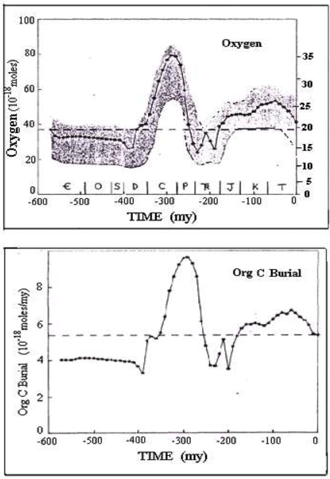
In equation (4) the biomass is presented by two parts. The first part is the biomass of currently living organisms. The corresponding portion of the oxygen released into the atmosphere. The second part of the biomass corresponds to the buried organic matter, which in the past was “living matter”. Oxygen, which corresponds to this part of the biomass converted into sedimentary organic matter, was released in the photosynthesis reaction, when corresponding organisms were alive. This oxygen has accumulated in the atmosphere. The validity of using the photosynthesis equation for the global carbon cycle is confirmed by two correlations of natural parameters. The first corresponds to the “substrate – product” relationship stemmed from photosynthesis equation. One can see the expected counter-phase correlation between time-averaged changes of CO2 and O2 concentrations in the atmosphere, obtained from model calculations in the Phanerozoic (Fig.1). The second correlation corresponds to the “product –product” relationship from photosynthesis equation (Fig.2)

GEMS-2020-101_Ivlev AA_F1

Figure 1. Changes in the atmospheric concentration of CO2 (solid line) and O2 (dashed line) during Phanerozoic eon. Abbreviation of the periods: S – Silurian, D – Devonian, C – Carboniferous, P- Permian (Palaeozoic era); Tr – Triassic, J – Jurassic, K – Cretaceous (Mesozoic era); Pg – Palaeogene and Ng – Neogene (Cenozoic era). Given that the reaction is of the first order, one can expect an antiphase link between CO2 and O2. The first two periods of Palaeozoic era (Cambrian and Ordovician) are not shown because there is some uncertainty around establishing the CO2 and O2 concentrations. CO2 estimates are from the Geocarb III model (Igamberdiev, Lea, 2006).

GEMS-2020-101_Ivlev AA_F2

Figure 2. The in-phase changes of oxygen content in the atmosphere and burial organic matter rates in the sedimentary rocks in Phanerozoic. The shaded zone for oxygen designates the zone of possible errors based on sensitivity analysis (Berner & Canfield, 1989).

One can see the expected syn-phase correlation between oxygen growth in the atmosphere and the increase in the mass of buried carbon (mol/million years) in the same time interval. Moreover, one can conclude that it is possible to neglect the biomass that corresponds to “living matter” as compared with buried organic matter. Following this approximation, the equation of photosynthesis for global carbon cycle can be simplified like that:

GEMS-2020-101_Ivlev AA_F7

To use the term “global photosynthesis” in carbon cycle studies effectively, it is important to understand what properties of traditional photosynthesis could be applied to the global photosynthesis, according its definition [3]. The most important property is the presence of two reciprocally related processes – assimilation of CO2 and photorespiration. Besides, an increase in the concentration of CO2 in the environment strengthens the assimilation function, while an increase in the concentration of O2 in the atmosphere increases photorespiration. Therefore the CO2/O2 ratio is the important characteristic of the global carbon cycle. The growth of this ratio in the atmosphere causes sedimentary organic matter accumulation in the earth’s crust. In periods when the ratio drops, the organic matter content in the crust decreases. Like traditional photosynthesis, global photosynthesis is accompanied by isotopic fractionation. Notably CO2 assimilation and photorespiration are accompanied by the effects of the opposite sign. Increased CO2 assimilation (due to CO2

concentration growth) is accompanied with the enrichment of the biomass in light isotope 12С, while the strengthening of photorespiration (due to growth of O2 concentration) is accompanied by enrichment of the biomass with heavy isotope 13С. Unlike traditional photosynthesis, global photosynthesis does not have the capacity to ontogenetic changes. In addition to the features above mentioned, there are two important features of global photosynthesis, related to its participation in global carbon cycle. First is cyclicity, which is determined due to participation of global photosynthesis in orogenic cycles as their main element. Orogenic cycles, as known, are caused by the periodically recurring movement of lithospheric plates what leads to periodic injections of CO2 into the “atmosphere – hydrosphere” system. The combination of lithosphere plates’ motion with photosynthesis development provides climatic changes. The latter causes biotic turnover. Indeed, each orogenic cycle begins with low oxygen and high CO2 conditions and is completed with the inverse ratio of these parameters. Drastic climatic changes cause biotic turnover. The repetition of these cycles leads to natural selection, consolidation of useful properties and adaptability of organisms in different environment. It was manifested in the structural and chemical features of organic matter and oils observed in the course of evolution. Actually, each photosynthetic cycle begins with low oxygen and high CO2 conditions and completing with the inverse ratio of these parameters. It resulted in drastic climatic change causing mass extinction. The repetition of these cycles leads to natural selection, consolidation of useful properties and adaptability of organisms in different environment. The second important feature of global photosynthesis is spontaneous striving to a stationary state. It is a manifestation of the ability of each individual photosynthesizing organism to enhance the photorespiration in response to the increase of oxygen content in the environment. It goes on until the amount of the evolved carbon becomes equal to the amount of the assimilated carbon. This state is called ecological compensation point. It determines the boundaries of the physical survival of the organisms. It was also shown that a set of plants, placed in the closed camera, where photosynthesis occurs, in some time make the atmosphere in the camera stable [4], [5] conjectured that land plants are responsible for the equilibration of the atmosphere on the Earth. Developing this idea in respect to carbon cycle, we suggested the ecological compensation point concept. Taking into account that from the photosynthesis origin the oxygen content in the atmosphere steadily increased (Table 1) we believed that it went on up to the moment when biomass produced in photosynthesis became equal to the amount of organic matter oxidized to CO2 in the course of carbon turnover. We called this state the ecological compensation point. When the system achieved this state, all the processes in it became stationary and began to oscillate around some steady state level.

Table 1. Estimates of the average concentrations of O2 in the atmosphere during geological time, obtained by different models.

Eon / Era
Numerical age
Ma

Approximate
value

References

Precambrian/ Paleoproterozoic

2200 – 2000

~ 0,2 %

Holland 1998[7,8]; Bjerrum, Canfield, 2004 [9]

Precambrian/ Neoproterozoic

1700 – 570

2 – 3 %

Canfield, Teske, 1996 [10]

Phanerozoic/ Cambrian– Devonian

570 – 350

< 15 – 17 %

Berner, Canfield, 1989 [11]; Berner et al, 2000 [12]; Berner, 2003[13]

Phanerozoic/Carboniferous– Permian

350 – 230

25 – 30 %

Lenton, 2001[14]

Phanerozoic/ Mezozoic Triassic – Cretaceous

 230 – 145

20 %

Lenton, 2001 [14]; Bergman et al., 2004 [15]

Phanerozoic / Cenozoic / Neogene / Miocene

23

23 %

Berner [16], Kothavala, 2001 [17]

It was found this point was achieved in Miocene when new type of CO2 assimilation, called C4-type, has appeared [6]. Since this moments the regulation of the CO2/O2 ratio and the associated processes turned to be under the control and began to realize through the change in the ratio of C3/C4 type plants. The last feature of global photosynthesis has a very deep physical sense. Indeed, when the system became steady state it has become very unstable and dependent even on weak external impacts. Simultaneously many important vital parameters of the system, such as O2 and CO2 concentrations, surface temperatures, sea level, etc., which critical to humanity existence, has become unstable too. It makes people to follow closely variations of parameters to counter threats. From the stationary state of the global carbon cycle one can deduced that the amount of carbon produced in photosynthesis is approximately constant. Hence the amount of hydrocarbons produced by organic matter should be approximately constant too, as well as the amount of generated petroleum. Considering the steady state of oil reproduction and the ever increasing volume of its consumption, the expression that oil is a non-renewable resource acquires obvious sense.

Conclusion

  1. The term “global photosynthesis” is necessary to describe photosynthesis in large systems such as the biosphere or the global carbon cycle. On the basis of the equation of traditional photosynthesis, approximations were obtained that describe the “substrate – product” and “product – product” relationships in photosynthesis for the large systems, like biosphere and global carbon cycle.
  2. It is shown that to study the changes occurred during the evolution of the global carbon cycle, in particular, for the identification of orogenic cycles, it is possible to use such features of traditional photosynthesis as the dependence of photosynthesis products on environmental conditions, as features of carbon isotope fractionation and others features, excepting ontogenetic ones
  3. The features of global photosynthesis associated with participation in the global carbon cycle, such as cyclicality and spontaneous striving to a stationary state with oxygen growth in the environment, are of special interest. The first is responsible for natural selection and fixation of useful properties in the course of evolution, including the ability to adaptation, A spontaneous approach of the system to a stationary state, called ecological compensation point, means that eventually the system will reach it. This state is very unstable and is sensitive to weak external impacts. Therefore, such vital parameters of the system, as the oxygen and carbon dioxide content in the atmosphere, the associated surface temperature on the Earth, sea level and many others are unstable as well and should be monitored. That’s why the numerous environmental problems inevitably arise and humanity needs to solve them to survive.
  4. Following the logic of stationary state one can conclude that in position of ecological compensation point the reproduction of sedimentary organic matter becomes steady state as well. Given that oil generation makes up a certain portion of sedimentary organic matter and taking into account that oil consumption is steadily increases it become evident that it is high time to think what should replace the oil disappearing.

References

  1. Vernadsky VI (1926) Isotopes and “living” matter. Dokl.
  2. Ivlev AA (2019) The Global Carbon Cycle and the Evolution of photosynthesis. Cambridge Scholars Publishing.
  3. Ivlev AA (2019) Functions of Global Photosynthesis. AS Agriculture 3: 23–24.
  4. Jahren AH, Arens NC, Harbeson SA (2008) Prediction of atmospheric δ13CO2 using fossil plant tissues. Rev Geophys 46.
  5. Tolbert NE, Benker C, Beck E (1995) The oxygen and carbon dioxide compensation points of C3 plants: Possible role in regulating atmospheric oxygen. Proc Natl Acad Sci 92: 11230–11233. (Crossref)
  6. Cerling TE, Harris JM, MacFadden BJ, Leakey MJ, Quade J, et al. (1997) Global vegetation change through Miocene/Pliocene boundry. Nature 389: 153–158.
  7. Holland HD (1965) The history of ocean water and its effect on the chemistry of atmosphere. Proc Natl Acad Sci USA 53: 1173–1183. (Crossref)
  8. Igamberdiev AU, Lea PJ (2006) Land plants equilibrate O2 and CO2 concentrations in the atmosphere. Photosynthesis research 87: 177–194. (Crossref)
  9. Bjerrum CJ, Canifield DE (2004) New insight into the burial history of organic carbon on the early Earth. Geochim Geophys Geosyst 5.
  10. Canfield DE, Teske A (1996) Late Proterozoic rise in atmospheric oxygen inferred from phylogenetic and sulphur-isotope studies. Nature 382: 127–132. (Crossref)
  11. Berner RA, Canfield DE (1989) A new model for atmospheric oxygen over Phanerozoic time. Am J Sci 289: 333–361. (Crossref)
  12. Berner RA, Petsch ST, Lake JA, Beerling DJ, Popp BN et al. (2000) Isotope fractionation and atmospheric oxygen: implications for Phanerozoic O2 evolution. Science 287: 1630–1633.
  13. Berner R (2003) The long-term carbon cycle, fossil fuels and atmospheric composition. Nature 426: 323–326. (Crossref)
  14. Lenton TM (2001) The role of land plants, phosphorous weathering and fire in the rise and regulation of atmospheric oxygen. Global Change Biol 7: 613–629.
  15. Bergman MJ, Lenton TM, Watson (2004) AG COPSE: a new model of biogeochemical cycling over Phanerozoic time. Am J Sci 304: 397–437.
  16. Berner RA (1999) Atmospheric oxygen over Phanerozoic time. Proc Natl Acad Sci USA 96: 10955–10957. (Crossref)
  17. Berner RA, Kothavala Z (2001) GEOCARB III: a revised model of atmospheric CO2 over Phanerozoic time Am J Sci 301: 333–361.

Higher Maternal Death Rates Occur in Rural United States and Illinois

DOI: 10.31038/AWHC.2020312

Introduction

Nationally and internationally, maternal mortality is an important indicator of the quality of a nation’s healthcare [1]. Recent statistics reported by the Centers for Disease Control and Prevention (CDC) indicates an increase in the pregnancy-related maternal mortality ratio (MMR) to 17.0 deaths per 100,000 live births from 2011–2013 [2], while  in Europe and maternal death rates are declining [3,4]. When analyzing the demographics of maternal deaths in the U.S., it appears pregnancies in rural environments are more at risk, with some maternal mortality rates in rural areas as high as 28.7 deaths per 100,000 live births [5]. A study by Kozhimannil and colleagues [6] demonstrated a rise in the maternal mortality and morbidity of both rural and urban areas, but rural mothers had a 9% greater chance of an adverse outcome compared to the urban mothers. The WHO has identified several factors that account for 75% of all maternal deaths: severe bleeding and infections after childbirth, pre-eclampsia and eclampsia, complications from delivery, and unsafe abortion [7]. The majority of these conditions could be prevented if recognized and treated by a skilled medical professional and if birth takes place in a sanitary place early enough (e.g. hospital), which can be difficult if the patient lives in an area with a shortage of skilled healthcare providers or a long distance from these professionals, as is often the case in rural settings. The purpose of this article is to examine the differences in maternal death rates between rural and urban Illinois stratified by urbanization level and race/ethnicity from 2007 to 2016.

Methods

Maternal death rates per 100,000 women ages 15 through 54 were obtained from the CDC Wonder website for years 2007 to 2016. This age range was chosen to include a larger sample size who are still capable of child-bearing and whose cause of death was within the pregnancy categories of ICD-10 (O00 to O99). This data was further stratified into six urbanization categories defined by the Office of Management and Budget and National Center for Health Statistics: large central metro, large fringe metro, medium metro, small metro, micropolitan, and non-core. A literature search using PRISMA guidelines was conducted using the term “maternal mortality” and keywords “community” and/or “neighborhood.” Studies were limited to those written in English. Maternal death rates per 100,000 women ages 15 through 54 for the various subgroups were calculated using the CDC Wonder website, and statistical comparison of rates was done using methods described by Dever [8].

Results

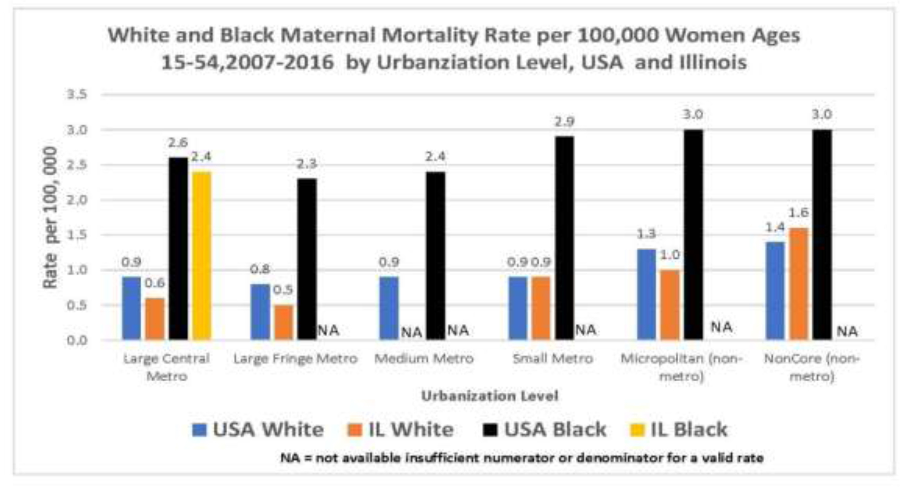
Maternal death rates were first analyzed by urbanization categories for all races for the U.S. compared to Illinois (Graph 1). The only statistically significant difference was found in the large fringe metro category with Illinois having a significantly lower maternal death rate than the U.S. Other than small metro, all other urbanization categories had lower maternal death rates than the U.S. When these urbanization categories were broken down into racial/ethnic subgroups, White mothers in both Illinois and the U.S. as a whole were found to have statistically significant higher maternal death rates in the micropolitan and non-core categories (rural) when compared to the large central metro category. The Illinois white non-core rate was at least twice that of the four most urban areas. Maternal deaths for African American mothers in Illinois were too low to calculate a valid rate for rural areas, but U.S. African American maternal deaths are on average about 2.5 times than that of the U.S. Whites.

AWHC 2020-302-Erin Hinkley_F1

Graph 1

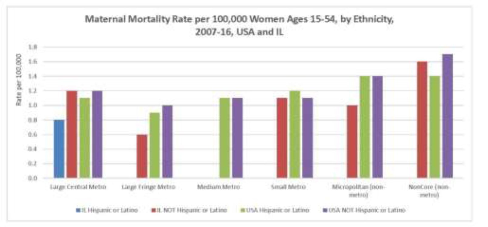
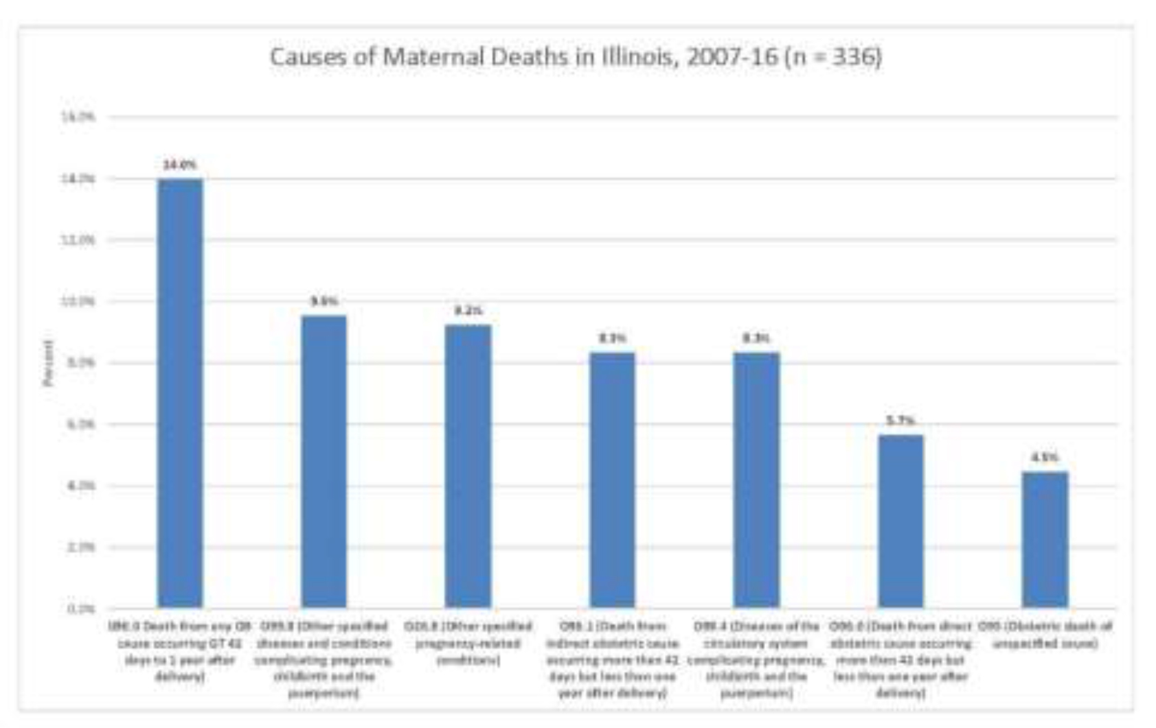
A gradual increase in maternal death rates within both Hispanics and non-Hispanics was observed as urbanization decreased, as the area became more rural (Graph 2). When comparing the large central metro U.S. non-Hispanic mothers to those in non-core areas, the more rural mothers had a statistically significant higher maternal death rate. Regarding the causes of maternal death according to ICD-10 codes. Any obstetrical complication from 42 days to a year postpartum (O90.0) was the most common coded caused of death at 14% (Graph 3). Overall about 28% of maternal deaths, both indirectly and directly related to an obstetrical cause, occur greater than 42 days but less than a year postpartum.

AWHC 2020-302-Erin Hinkley_F2

Graph 2

AWHC 2020-302-Erin Hinkley_F3

Graph 3

Discussion

White mothers residing in rural areas have higher maternal death rates when compared to all other mothers. These maternal deaths negatively impact the health and future outcomes of the infants left motherless in addition to financially impacting the families due to medical costs. About one-third of maternal deaths occur 42 days postpartum; literature suggests these deaths may be due to life-threatening bleeding and infections, blood pressure elevations, complications from childbirth, and unsafe abortions [7]. Kozhimannil and colleagues [9] attribute the patterns seen in rural areas to the loss of obstetrical care in rural settings, requiring mothers to travel in order to safely deliver their babies. Future studies should focus on determining the specific clinical causes of maternal death in rural areas in order to develop interventions to reduce and prevent maternal death. The limitations within this study lie partially in the dataset from the CDC. The data assumes the causes of maternal death are correctly coded on the death certificate; incorrect coding would alter the death rate from its true value. Maternal mortality rates would have been a more precise measure as it uses the number of women who gave birth as the denominator rather than the number of women in that specific subgroup. Some data was limited due to low population numbers in different subgroups; maternal death rates for Hispanic mothers in Illinois could only be calculated in the large central metro area as the numbers were too low in the less urban categories. A future study should aim to investigate the causes of the very elevated Black maternal death rate in Illinois as well as the U.S. Other studies may investigate maternal death patterns according to age, education level, access to pre- and post-natal care, and the experience of the delivering provider in those areas. These findings may help stimulate improvements where shortfalls lie in order to provide the best care to mothers as possible.

In conclusion, this study shows substantially elevated maternal death rates for mothers residing in rural areas relative to urban areas and serves as basis to advocate for systematic changes in those areas whose mothers are at the highest risk.

References

  1. MacDorman MF, Declercq E, Cabral H, Morton C (2016) Recent increases in the U.S. maternal mortality rate: Disentangling trends from measurement issues. Obstet Gynecol 128: 447–455. [crossref]
  2. Creanga AA, Syverson C, Seed K, Callaghan WM (2017) Pregnancy-related mortality in the united states, 2011–2013. Obstet Gynecol 130: 366–373. [crossref]
  3. MacDorman MF, Declercq E, Thoma ME (2017) Trends in maternal mortality by sociodemographic characteristics and cause of death in 27 states and the District of Columbia. Obstet Gynecol 129: 811–818. [crossref]
  4. United nations millennium development goals. http://www.un.org.proxy.cc.uic.edu/millenniumgoals/. Accessed Mar 29, 2018.
  5. Meyer E, Hennink M, Rochat R, et al. (2016) Working towards safe motherhood: Delays and barriers to prenatal care for women in rural and peri-urban areas of georgia. Matern Child Health J 20: 1358–1365. [crossref]
  6. Kozhimannil KB, Interrante JD, Henning-Smith C, Admon LK (2019) Rural-urban differences in severe maternal morbidity and mortality in the US, 2007–15. Health Affairs 38: 2077–2085.
  7. WHO | maternal mortality. WHO Web site. http://www.who.int.proxy.cc.uic.edu/mediacentre/factsheets/fs348/en/. Accessed Mar 29, 2018.
  8. Dever GEA (1991) Community health analysis: Global awareness at the local level. 2nd ed. Gaithersburg, Md: Aspen Publishers.
  9. Kozhimannil KB, Hung P, Henning-Smith C, Casey MM, Prasad S (2018) Association between loss of hospital-based obstetric services and birth outcomes in rural counties in the united states. JAMA 319: 1239–1247.

Experimenting & learning to think critically and competently: Combining 2020 technology with student-driven research

DOI: 10.31038/PSYJ.2020214

Introduction

One might not think that the ubiquitous availability of cheap, easy, powerful computing power combined with storage and retrieval of information would produce in its wake better students, better minds, and the benefits of better education. The opposite is the case. As the increasing penetration of consumer electronics continues apace, it is becoming increasingly obvious that students have neither the patience to pay attention, nor the ability to think critically.  A good measure of that loss of student capability comes from the popular press, where blog after blog decries the loss of thinking and, in turn, the power of education. Not to be outdone, the academic press as signaled by Google Scholar ® provides us with a strong measure of this electronics-driven loss of thinking and withering of education. Table 1 shows the year by year data.

Table 1. Concern with the loss of critical thinking – a 10-year count (Source: Google Scholar®)

Year

Loss of critical thinking

Experiential Learning

2010

9,970

51,300

2011

11,800

53,700

2012

12,300

58,100

2013

13,800

61,400

2014

14,000

62,000

2015

15,800

57,500

2016

15,300

48,000

2017

17,200

47,200

2018

17,100

39,300

2019

9,800

30,100

How then can we make education more interesting?  This paper is not a review of attempts to make education more involving, more interesting, but rather presents a simple, worked approach to making learning more interesting, but really far deeper. It is obvious that children like to talk to each other about what they are doing, to present information about their discoveries, their developments, themselves. Children like experiences which resemble play, in which they are somewhat constrained, but not very much. And when a child discovers something new, something that is his or hers, the fun is all the greater because the discovery can be shared. The ingoing assumption is that if learning can be made fun, a game, with significant outputs of a practical nature, one might stimulate a love of learning which love seems to have disappeared.

Experiential learning and discovery of the new – A proposed approach based upon the emerging science of Mind Genomics

The emerging science of Mind Genomics can be considered as a hybrid of experimental psychology, consumer research, statistics, and mathematical modeling. The objective of Mind Genomics is the study of how people respond to the stimuli of the ordinary, the every day. We know from common experience that people go about their daily business almost without deeply thinking about things, in a way that Nobel Laureate Daniel Kahneman called System 1, or ‘thinking fast’ [1]. We also know that there are many different aspects to the same experience, such as shopping. People differ, consistently so, in when they shop, why they shop, how they get to the place where they will make a purchase, the pattern of shopping, what they shop for, and why.  The variation is dramatic, the topics not so interesting, the exploration of the topics left to mind-numbing tabulations, which list the facts, rather than penetrating below, into the reasons.

Mind Genomics was developed to understand the patterns of decision making, not so much in artificial laboratory situations to develop hypotheses for limited situations, but rather to understand the decision rules of daily life.  Instead of mind-numbing tables of statistics from which one gleans patterns, so-called ‘connecting the dots,’ Mind Genomics attempts to elicit these individual patterns of decision making in easy-to-do experiments.  The output, once explained, fascinates the user, converting that user into an involved explorer, looking for novella, insights, and discoveries that are new to the world, discoveries ‘belonging to the student’. The day to day worlds, the ordinary, quotidian aspects of our existence, become grist for the mill of discovery. The result is that discoveries about the ordinary, discoveries that when harnessed by teachers and appreciated by students, combine experiential learning, and learning how to think critically

As noted above, Mind Genomics derives historically from psychology, consumer research, statistics, and modeling. The objective of Mind Genomics is to uncover the specific criteria by which people assign judgments. The topics are unlimited.

The empirical portion of this paper will show how experiential learning and critical thinking may be at the fingertips, with the use of simple computer programs, specifically BimiLeap, freely accessible at www.BimiLeap.com.  In this paper we look at how a 14-year-old student can learn about laws and ethics, as well as the issues of daily life. The topic is taken from the way young students in a Yeshiva, a rabbinic school, can learn about the issues underlying property, specifically borrowing property and what happens when the property is somehow ‘lost.’

Experiential learning and discovery of the new

A proposed approach based upon the emerging science of Mind Genomics.  Mind Genomics is an emerging science combining experimental psychology, consumer research, experimental design, and statistical modeling. The objective is to explore decision making in the everyday world.

In terms of commercial and social practice, Mind Genomics has been applied in by author HRM to issues as varied as it applies to topics as different as decision making about what we choose to eat, legal cases, and communications in medicine to improve the outcomes during and after hospitalization, respectively. These practical applications along with the ongoing stream of studies suggest Mind Genomics as a simple-to-use but powerful knowledge-creation tool. With Mind Genomics, virtually anyone can become a researcher, explore the world, classify the strategies of decision making, and discover new-to-the-world mind-sets, groups of people who think about the topic in the same way, and who differ from other groups of people thinking about the topic in a different way.

The Mind-Genomics technology has been embedded in easy-to-use computer programs, making the typical Mind Genomics study fast, affordable, and structured. The same simplicity of research, studying what is, may thus find application to educate the non-researcher, the novice, the younger student. Rather than the researcher exploring a topic area with the point of view of a person interested in the specific topic, the notion emerged that the same tool can be used to each a novice how to think, using research as a the tool, and the information and accomplishment as the reward for using the tool.

The Yeshiva approach: Havrutas (groups) studying a topic in depth

This paper presents one of the early attempts to use Mind Genomics to teach legal reasoning to a teenager, helping the teenager to make a specific topic ‘come alive’ as well as imbue experiential learning and critical thinking into the process.  The paper will present the approach step by step, as a ‘vade mecum’ or ‘guide’ for the interested reader.

The objective of Mind Genomics is to understand the decision making in a situation.  The deliverable is a simple table, which one can adorn in different ways, but which at its heart shows questions and answers about a situation.

We take our approach from the way students in Jewish religious schools study the corpus of Jewish law, commentary and discussion.  The notion of using the Bible as a source for teaching modern concepts is not new [3]. created a course on economics, based upon biblical tests, as described in the following paragraph

The author describes a course designed to build the critical thinking skills of undergraduate economics students. The course introduces and uses game theory to study the Bible. Students gain experience using game theory to formalize events and, by drawing parallels between the Bible and common economic concepts, illustrate the pervasiveness of game-theoretic reasoning across topics within economics as well as various fields of study.

We take our source for the course in the way the Talmud is study. The Talmud comprises more than 2700 of pages of explication of basic Jew practice.  The origins of the Talmud are, according to Jewish sources, founded in the Oral Law, the law of Jewish practice based in the Old Testament, the Jewish Bible, but expanded considerably.  For the reader, the important thing to know is that the Talmud comprises two portions, the Mishna, a short, accessible compilation of Jewish Law and practice, finalized by Rabbi Judah the Prince around the second century CE, and then discussions of that compilations, attempting to find discrepancies to reconcile them, done by Rabbis and their students for about 300–400 years hundred years after the Mishna was finished. This section, discussion and reconciliation among sources, is embodied in difficult, occasionally tortuous material known as the Gemara, the word in Aramaic for‘completing.’

Talmud students who spend years learning the Talmud end up thinking critically [4]. The method is to pair off students with each other, havrutas, usually comprising two students, who read, decipher, debate, and struggle to understand the section together. The approach leads, when successful, to logical thinking, and ability to formulate problems ina way worthy of a lawyer.  In the words of [5].

when examined closely, havruta study is a complex interaction which includes steps, moves, norms and identifiable modes of interpretative discussion [5].

Havruta learning or paired study is a traditional mode of Jewish text study. The term itself captures two simultaneous learning activities in which the Havruta partners engage: the study of a text and learning with a partner. Confined in the past to traditional yeshivot and limited to the study of Talmud, Havruta learning has recently made its way into a variety of professional and lay learning contexts that reflect new social realities in the world of Jewish learning [6].

With this very short introduction, the notion emerged from a number of discussions with psychology researchers and with students of the Talmud that perhaps one might use technology inspired by Talmudic style thinking and discussion to teach students to think critically, whether these be Talmud students embedded in the Jewish tradition, or students who could take a topic of the Talmud in an ‘edited’ form, and work with that topic in the way a yeshivastudent might.

Adapting the approach, making it accessible, challenging, interactive, and fun

The situation for this study is simple, based upon a legal case well known to many students of the Talmud, but presented in secular terms. The case concerns an item, the nature of which is unstated but the implication is that the item is something portable.  The information available is:

  1. Who initiated the interaction?
  2. Why was the interaction initiated?
  3. Where was the interactioninitiated (viz., request made)?
  4. What happened to the item?

In order to make the system easy, but keep the tone serious, the design for the computer interface was created to be simple. 

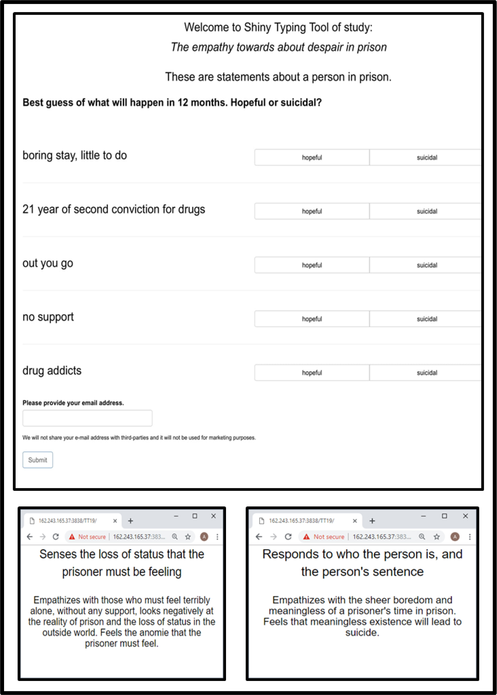
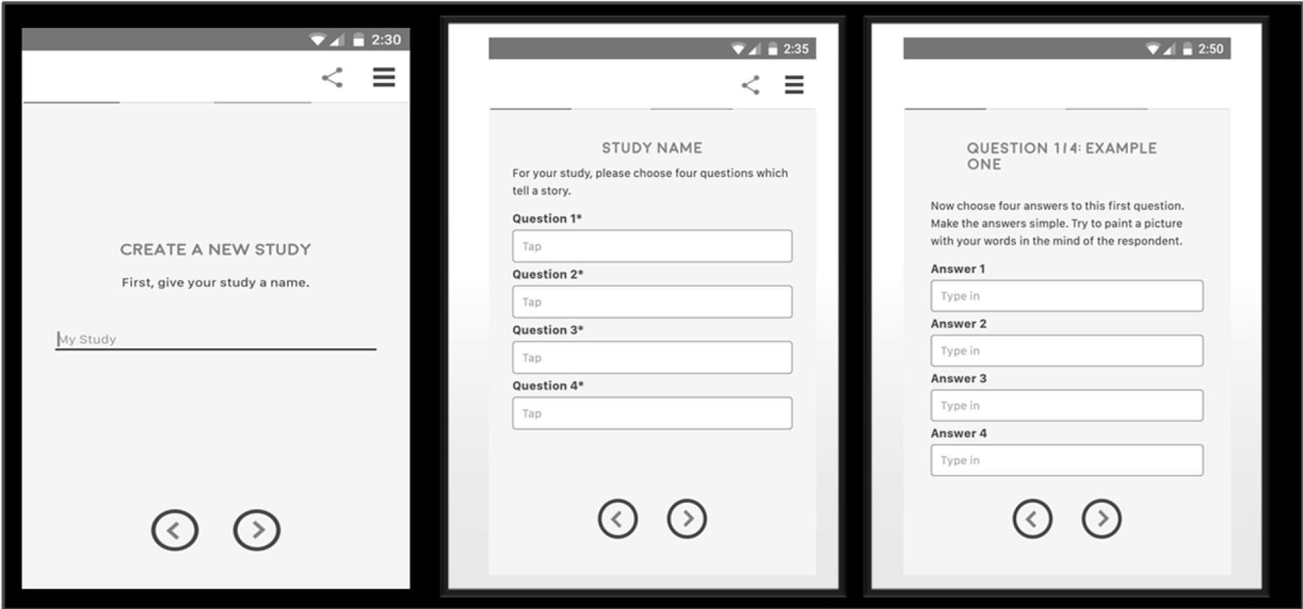
Figure 1 shows the three key screen shots.
Mind Genomics-039_F1

Figure 1. The setup showing the three panels which force the student to think in an analytic yet creative and participatory fashion

The left panel shows the requirement that the student(s) select a name for the study. It may seem simple, but it will be the name of the study which drives much of the thinking.

The middle panel shows the requirement to create four questions dealing with the topic, with the questions ‘telling a story.’ It is here, at this second stage, beyond the name of the topic, where students encounter problems, and must ‘rewire’ their thinking. Students are taught to understand, to remember, to regurgitate. Students are not taught to ask a series of questions to elucidate a topic.  Eventually, the students will learn how to ask these questions, but it will be much later, when the student is introduced to research in the upper grades, and when the student becomes a professional, especially a lawyer.  We are creating the opportunity to bring that disciplined thinking to the junior high school or even to grade school.

The right panel shows the requirement to provide four answers to one of the questions. There is no hint, no guidance, about what the answers should be, but simply the question repeated to guide the student.  Typically, this third panel is easy to complete once the student has gone through the pain of thinking through the four questions. That is, the questions are hard to formulate; the answers are easy to come by after the hard thinking has been done.

Engaging the student in the creation of questions and answers

The key to the approach is the set of questions, and secondarily the set of answers. As noted above, the demand on the participant is to conceptualize the topic at the start, rather than being trained to deconstruct the topic when it is fully presented.  The approach thus is synthetic, requiring imagination on the part of the student. 

Table 2 presents the four questions and the four answers to each question.  The questions and the answers do not emerge simply from the mind of the student, at least not at first. There are the inevitable false steps, the recognition that that the questions do not make sense, do not tell a story, do not flow to create a sequence, etc.  These false steps are not problems, but rather part of the back and forth learning how to reason, how to tell a coherent story, and how to discard false leads.

Table 2. The four questions, and the four answers to each question

Question 1 – Who initiated?

A1

Initiated by:  Young neighbor (14 years old)

A2

Initiated by: Older neighbor (29 years old)

A3

Initiated by: School friend in high school

A4

Initiated by:  Uncle of person

Question 2 – What was the action

B1

Action: To borrow item for use in project

B2

Action: To use item as part of a charity event

B3

Action: To guard item while the owner went away

B4

Action: To try to sell the item at a garage sale

Question 3 – How or where was the request made?

C1

Request made: On telephone

C2

Request made: In a group meeting

C3

Request made: In a house of worship

C4

Request made: At a dinner party

Question 4 – What eventually happened?

D1

What eventually happened: Item lost

D2

What eventually happened: It destroyed in accident

D3

What eventually happened: Item stolen on bus

D4

What eventually happened: Item given away by error

The answers in Table 2 are simple phrases, with the introduction to the answer being a phrase to reinforce the story.  Various efforts at making the approach simply continue to reveal that for those who are beginning a topic, it is helpful to consider the answers as continuations of the questions. That specification, such as ‘initiated by’ will also make the respondent’s effort easier.

It is important to keep in mind that the process of topic/question/answer will become smoother with practice, the topics will become more interesting, the questions will move beyond simple recitation of the order of events, and the answers will become more like a literary sentence, and less like a menu item.

In the various experiences with this system, it is at this point, the four questions, that most people have difficulties. Indeed, even with practice, people find it hard to organize their thinking to bring a problem into sufficiently clear focus that they can make it into a story. When the researcher finally ‘understands the task’ the response is often a statement about ow they feel their ‘brains have been rewired.’ Never before did the researcher have to think in such a structured, analytic way, yet with no guidance about ‘what is right.’

One of the more frequent questions asked at this point is ‘Did I do this right?’  Most people are unaccustomed to structured thinking.  After creating the questions, and on the second or third effort, after the first experiment, the researcher begins to feel more comfortable, and is able to move around the order of questions, changing them to make more sense. This flexibility occurs only after the researcher feels comfortable with the process.

Creating ‘meaningful’ stimuli by means of an underlying experimental design

As students, we are typically taught the ‘scientific method,’ namely to isolate a variable, and understand it.  Our mind is attuned to dissecting a situation, focusing on one aspect.  We lose sight of the fact that the real world comprises mixtures, and that an understanding of the real world requires us to deal with the way mixtures behave.  An observation of our daily actions quickly reveals that virtually all of the situations in which we mind ourselves comprises many variables, acting simultaneously.  Indeed, much of the problem of learners is their experienced difficulties in organizing the multi-modal stimuli impinging on themand learning to focus and to prioritize.  It is to this skill we now turn as we look at the student experience.

The computer program combines alternative answers to these four questions, creating short vignettes, presents them to respondents, gets a rating of ‘must repay’ vs ‘does not need to repay’.’

The above-mentioned approach seems, at first glance, to be dry, almost overly academic. Yet, the Mind Genomics approach makes the ‘case’ into something that the students themselves can create, investigated, and report, with a PowerPoint® presentation of the study, something that will be part of their portfolio for life, and can be replicated on many different topics.

Each respondent evaluates a unique set of vignettes, created by a systematic permutation of the combinations. The mathematical rigor of the underlying experimental design is maintained, but the different combinations ensure that across all the respondents a wide number of potential combinations are evaluated.

The underlying experimental design and indeed all of the mathematics for the analysis are shielded from the respondent, who is forced to ‘think’ about the topic, and the meaning of the data, rather than getting lost in deep statistics. 

The composition of the vignettes is strictly determined by an underlying specification known as an experimental design [7]. Each vignette comprises either two, or three or four answers, at most one answer from a question, but sometimes no answer from a question.  The experimental design ensures that the 16 elements appear as statistically ‘independent of each other,’ so knowing that one answer appears in a vignette does not automatically tell us whether another answer will appear or not appear.

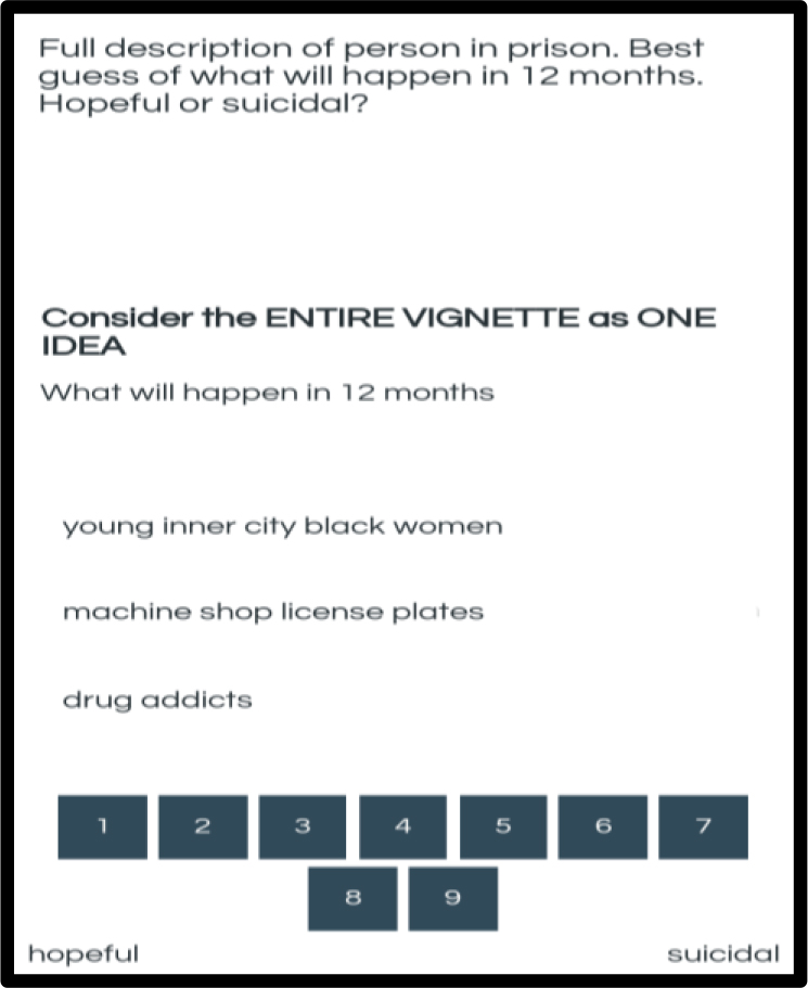
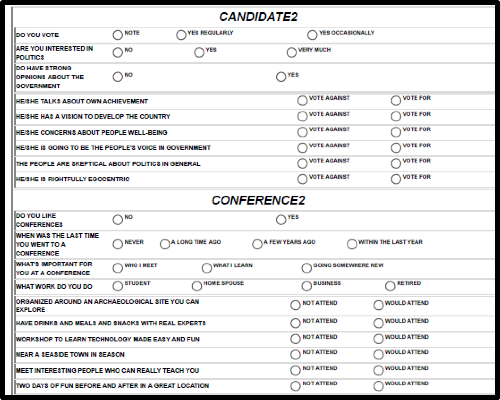
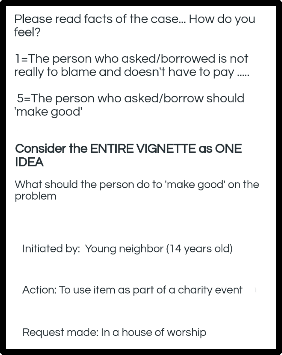
Figure 2 shows an example of a vignette created according to the underlying design.  The respondent does not know that the computer has systematically varied the combinations.The vignette is created by an underlying experimental design which prescribes the composition of each vignette.  Each respondent evaluates 24 different vignettes, or combinations of answers, and answers only. No questions leading to the answers are presented directly, although for this case the question is embodied at the beginning of the answer.
Mind Genomics-039_F2

Figure 2. Example of a vignette comprising three answers or elements, one answer from three of the four questions. Most vignettes comprise four answers, some comprise three answers, and a few comprise two answers.

An important challenge in Mind Genomics is to come up with a meaningful rating question. The rating question links the test stimuli, our vignettes, and the mind of the respondent.  Without a meaningful test question all we have are a set of combinations of messages.  The test question focuses the respondent’s mind on how to interpret the information in the vignette.

The test question is posed simply as either a unipolar scale (none vs a lot) or a bipolar scale (strong on one dimension vs strong on the opposite dimension, such as hate/love).  To the degree that the researcher can make the rating question meaningful, the researcher will have added to the power of the Mind Genomics exercise.

Our topic here concerns the loss of property occasioned by one person giving property to another person, after being asked to do so, or after being motivated to do so, that motivation coming from within.  A reasonable rating question is whether the person in whom the property is placed, for whatever reason, is required to ‘make good byreplacing the property’ or ‘not required to replace the property.’  Rather than requiring a yes/no answer, we allow the respondent to assign a graded value, using a Likert Scale:

1  =   The person who asked/borrow is not really to blame and doesn’t
          have to pay ….

5  =   The person who asked/borrowed should ‘make good.’

The phrasing of the question and the simple 5-point rating scale make the evaluation easy, and remove the stress from the respondent. By allowing the student a chance to assign a graded rating, the student can begin to understand gradations of guilt and innocence. Furthermore, the answers are not so clear cut, so straightforward that they prevent the student from thinking.  The requirement to take the facts of the case into account and rate the feeling of guilt vs innocence on a graded scale forces the student to think.  The very ‘ordinariness’ of the case encourages the student to become engaged, since the case is something that no doubt the student has either experienced personally, or at least has heard about at one or another time.

Obtaining additional information from the respondent

Quite often, those who teach do not pay much attention to WHO the respondent actually is, or even the different ways that people think. The academies where the Talmud was created did pay attention to the way people think, coming up with different opinion about the same topic. These different opinions were enshrined in discussions. The intellectual growth coming from thinking about the problem was maintained over the millennium and a half through the discussions of students about different points of a topic, and the study of those who commented on the law, and gave legal opinions about cases. The back and forth discussions about why the same ‘facts on the ground’ would lead to different opinions became a wonderful intellectual springboard for better thinking.  Few people, however, went beyond that to think, in a structured way about how ordinary people might think of the problem, people who were not trained as legal scholars, nor empaneled in a judicial panel.

Part of the effort of the Mind Genomics project is to show to the student the way different people think about the topic, and how there is not necessarily ‘one right answer.’  Thus, at the start of the experiment, before the evaluation of the 24 vignettes by the respondent, the respondent is asked three questions:

  1. Year of birth, to establish age
  2. Gender
  3. A third question, chosen by the researcher. Here is the third question for this study.

How do you feel about mistakes that are made in everyday life, by ‘accident’

1=I believe that the law is the law 2=I believe in being lenient 3=I want to know the facts of the case more

Running the study for educational purpose – Mechanics

During the past several decades, and as the Mind Genomics technology evolved and was refined, a key stumbling point, i.e., a ‘friction point’ in today’s language, continued to emerge. This was the deployment of the study in a way that could be quick, inexpensive, and thus have an effect within a short time. Two decades ago as the Internet was being developed, a great deal of the effort of a Mind Genomics study was expended getting the respondents to participate, typically by having them come into a central location, such as a shopping mall, and spending ten or 15 minutes.  The result was slow, and the pace was such that it would not serve the purposes of education. The process was slow, tedious, expensive, and not at all exciting to anyone but a serious researcher.

During the formative years of the technology, 2010–2015, efforts were put against making the system fast, with very fast feedback.  The upshot was that a study could be set up in 30 minutes or faster and deployed on the internet with simply a credit card to pay for the cost of respondents, usually about 3.00$ per respondent for what turned out to be a 4 minute study.  A field service, specializing in on-line ‘recruiting’ would provide the appropriate respondents, sending them to the link, and obtaining their completed, and motivated answers. The respondent motivation was there because they were part of the panel.

The mechanics were such that the entire study in the field would come back in less than one hour and one minute. The total analysis, including the preparation of the report in PowerPoint(r), ready for the student presentation, took less than one minute from the end of the field.  Figure 3 shows an example of the PowerPoint(r), expanded to the slide sort format, showing the systematic presentation of the results.

Mind Genomics-039_F3

Figure 3. Example of the PowerPoint® report for the study, shown inlide-sort format. The respondent receives the PowerPoint® report and the accompany Excel® data sheet one minute after the end of the data acquisition.The report is in color, and ‘editable.’

  1. The title page, showing the study name, the researcher, the date
  2. Information about the BimiLeap vision
  3. The raw material – elements, rating question
  4. How the data are analyzed, showing the transformation from a rating scale to a binary rating, as well as introducing the concept of ‘regression modeling’ …. This explanatory information is presented in a short, simplistic manner, yet sufficient to show the nature of mathematical (STEM) thinking
  5. Tables of data showing the results from the total panel, key subgroups
  6. Mind Sets – a short introduction to how people can think differently about the topic, and a short introduction to the calculations. Once again, the focus is on the findings, not on the method
  7. Results from dividing the respondents into two mind-sets and three mind-sets
  8. IDT – Index of Divergent Thought – showing how many elements have strong positive coefficients,   when the data are considered in terms of total panel, two mind-sets and three mind-sets, respectively. The IDT can be used to understand how well the researcher has ‘dived in’ to the topic, to uncover different ways of thinking about the topic. The IDT can be used to ‘gamify’ the research process, by providing an operationally defined, objective measure, of ‘winning ideas.’
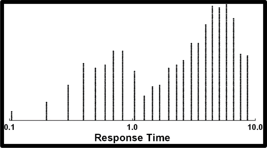
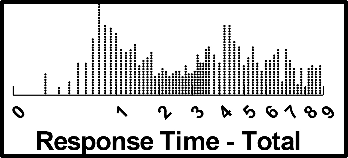
  9. Introduction to ‘response time’ – how long it takes the respondent to ‘process’ the ideas
  10. Tables of data showing the results from the total panel, key subgroups, and mind-sets
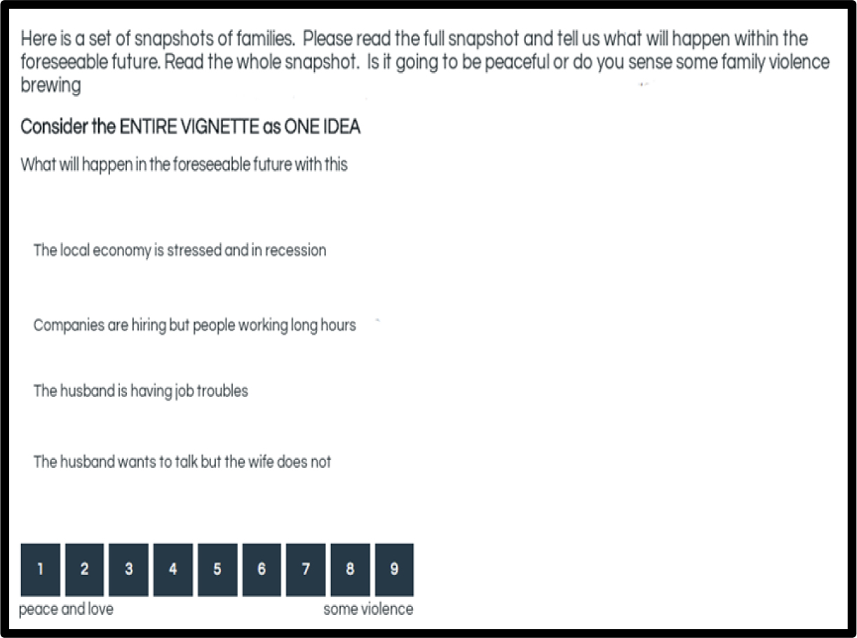
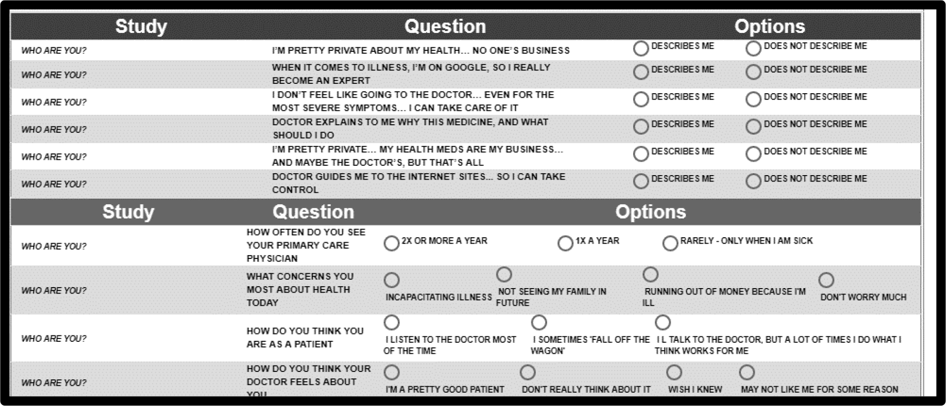
  11. Screen shots of the respondent experience

The report is accompanied by an Excel book with the data, set up for further analysis, if the student wishes.

The results, embedded in a pre-formatted PowerPoint® presentation, and with supporting full data in Excel®, are immediately dispatched by email and can always be retrieved from the researcher’s account, when, for example, the data are ‘updated’ with the ratings assigned by new panel participants. This process compresses the entire time, from set-up to data reporting, so that the results can be discussed within 1–3 hours after the official start the entire process, viz., entering the questions and answers into the BimiLeap programming and getting the panel provider to provide respondents.

The vision behind the PowerPoint® report is that it provides a tangible record of the student’s effort, a measure of what the student has achieved in the growth to learning.  By creating different groups of students who work together, and working together for 90 minutes in the afternoon, once per week, the typical student can generate 20–30 or so PowerPoint® in a year, a collection the quality of whose contents, study by study, will demonstrably improve as each study is designed, and executed with real people, the respondents.

What the student receives and how the student learns

Table 3 presents the unadorned results, a table.  To interpret the table is straightforward, despite the fact that it has simply numbers.  The researcher who is doing the study need not know the mechanics of how the numbers are computed, at least not in the beginning, in order to enjoy the benefits of Mind Genomics, and in order to participate in experiential learning.

Table 3. Output from a Mind Genomics on a simple legal case. The data is from the total panel


Found responsible and must make good

Total


Base Size

30


Additive Constant (Estimated percent of the times the initiator must repay in the absence of any information)

60


Question A: Who initiated


A2

Initiated by: Older neighbor (29 years old)

0

A4

Initiated by:  Uncle of person

-8

A1

Initiated by:  Young neighbor (14 years old)

-10

A3

Initiated by: School friend in high school

-10


Question B: What was the action


B2

Action: To use item as part of a charity event

5

B4

Action: To try to sell the item at a garage sale

-5

B1

Action: To borrow item for use in project

-6

B3

Action: To guard item while the owner went away

-11


Question C: Where was the request made


C1

Request made: On telephone

4

C2

Request made: In a group meeting

3

C3

Request made: In a house of worship

2

C4

Request made: At a dinner party

-2


Question D: What happened


D2

What eventually happened: It was destroyed in accident

6

D3

What eventually happened: Item stolen on bus

-8

D1

What eventually happened: Item lost

-10

D4

What eventually happened: Item given away by error

-10

The question what is the initiator (Question A) required to do.  At the low end, the initiator does not have to ‘make good’ (innocent, i.e., not pay.)  At the top end, the initiator has ‘make’ good (guilty, i.e., pay.)

Base Size: The table shows us that there are 30 different people who participated in the study. This is the base size.

Additive Constant: This is the expected number of times out of 100 people that the verdict will be ‘guilty’, i.e., must repay. What is special is that the additive constant is a baseline, corresponding to the likelihood that a person will say ‘guilty’ even in the absence of information. Our additive constant is 60. It means that when someone requests from another to do something with the item, 3 out of 5 (60%) the onus is on the person who does the requesting to take responsibility and pay if something happens to the item.

Coefficient: Ability of Each Element to drive Guilty (must repay). Let’s look at the power of Question A: Who initiated.  The four answers or alternatives, which appeared in the vignette, are either 0 (nothing) or negative. The negative means that when we know who initiated, we are likely to forgive. We forgive most when the action is initiated by a young neighbor or, or school friend in high school. The value is -10. That value -10 means the likelihood of guilty (must make good) goes from 60 (no information about the initiator) to 50, when the one piece of information about the initiator is presented as part of the case (specifically,  initiated by: School friend in high school.)  Of course, when the initiator is an older neighbor (29 years old), the coefficient is no longer -10 as it was before, but now 0. We (and of the course the student) have just discovered that it makes a difference WHO the initiator is. 

The same thinking can be done for the other questions and answers. Some, like D2 (What eventually happened: It was destroyed in accident) increase the likelihood of being judged responsible, and forced to make good, i.e., to repay.

The process from the vantage point of the researcher (e.g., the student)

As presented above, the process is simple, although quite uninteresting, except perhaps to the subject matter expert interested in lawor in thinking processes. How can the student be engaged to participate?  Otherwise, what we have here is simply another ‘dry process’ with some interesting but unexciting results.

The three aspects of the process are involvement, ease, and fast/clear results.  Absent those, and the process will remain in the domain of the expert, to be used occasionally when relevant, and otherwise to be relegated to process. The excitement of thinking and learning will not be experienced.

Let us proceed with the process.  The process follows a series of steps designed to make the researcher think. The process is structured, not particular hard after the first few experienced, but sufficiently challenging at the start so that the researcher realizes the intellectual growth which is taking place at the time of the research set up.

Experimental Designs – mixtures of answers

The actual test stimuli comprise mixtures of answer, without the questions. One can go to Table 2, and randomly pick out one answer from each of the four questions, present these answers together, on separate lines, and instruct the respondent to read the vignette, the combination, and rate the combination as a single entity.  The task may seem ‘strange’ to those who are accustomed to reading properly constructed paragraphs in their native language, but to those who are selected from random individuals to be study participants, there is no problem whatsoever. People follow instructions.   The problem with evaluating a few unconnected combinations is that there are no explicit patterns waiting to be discovery, and a discovery in turn which can teach systematic and critical thinking.

As noted above several times, the Mind Genomics paradigms works with an explicitly developed experimental design, which makes it easy for the equipped research to discover the pattern. Table 4 shows an example of the experimental design for a single respondent. There is a total of 16 answers and 24 vignettes, or combinations. The number and arrangement of the vignettes are not accidental, nor haphazard, and certainly not random, although it is tempting to say that the combinations are randomly arranged. Nothing could be further from the truth. The design, i.e., the combinations are precisely defined ahead of time , so that each of the 16 elements or answers appears exactly five time, that any vignette of combination has at most four answers (without their questions), that some combinations comprises two, others comprise three answers, and that the answers are systematically varied.  Finally, each of the experimental design is mathematically identical to every other design, but the specific combinations are different.

Table 4. The experimental design for 7 of the 24 vignettes for a respondent, as well as the rating, the binary expansion of the rating, and the consideration time

Order

A1

A2

A3

A4

B1

B2

B3

B4

C1

C2

C3

C4

D1

D2

D3

D4

Rating

Top2

7

1

0

0

0

0

0

0

1

0

0

0

1

0

0

0

0

4

100

8

0

0

1

0

0

0

0

1

0

0

1

0

0

1

0

0

1

0

9

1

0

0

0

0

0

1

0

1

0

0

0

0

0

0

1

3

0

10

0

1

0

0

1

0

0

0

0

0

1

0

0

0

0

1

5

100

11

0

1

0

0

0

1

0

0

0

1

0

0

0

0

1

0

3

0

12

0

0

1

0

0

0

0

0

0

0

0

1

0

0

1

0

3

0

13

0

0

0

1

0

0

0

1

0

0

1

0

0

0

0

0

3

0

Different points of view for the same argument – Mind-Sets and exciting discoveries

Students who ask questions to engage discussion are generally appreciated by their teachers. The questions show involvement.  Sometimes the questions spark lively discussions, especially when they are offered in the spirit of ‘looking at the problem in different ways.’

A foundation stone of Mind Genomics is the recognition and elicitation of different points of view about the same topic. The ingoing rationale is that in matters of everyday life there are facts, but often radically different opinions. Sometimes more learning emerges from the discussion of the topic from these different viewpoints than could ever emerge from rote learning of the ‘facts.’

One of the computations of Mind Genomics is the discovery of different mind-sets, groups of people with these individuals in one group looking at the topic differently from individuals in another group. The computational machinery of Mind Genomics enables these mind-sets to be discovered rapidly and inserted into the PowerPoint® report as simply new groups to consider and to discuss.

Table 5 shows the additive constant and coefficients for total (already discussed), gender, age, and two mind-sets. The students who participate in the study, indeed those who may have come up with the elements, can now see how the simplest of facts can be interpreted in different ways.

Table 5. The pattern of coefficients for ‘make good’, generated by key demographic groups (total, gender, age) and newly uncovered mind-sets.


Gender

Age

Mind-Set


Rating 4–5 transformed to 100;

Ratings 1–3 transformed to 0

Focus on ‘make good’ (guilty)

Tot

Male

Female

A16–19

A20–23

MS1

MS2


Additive constant (percent of times a rating will be 4–5 in the absence of any elements (i.e., a baseline)

51

53

66

40

63

56

48


Elements driving ‘guilty’ – Mind-Set 1

(Focus on action)


B2

Action: To use item as part of a charity event

10

-15

10

17

1

20

-5

B1

Action: To borrow item for use in project

5

-13

5

11

-4

16

-15

C1

Request made: On telephone

-2

0

-6

1

-6

11

-18

B4

Action: To try to sell the item at a garage sale

0

-25

-11

14

-16

10

-17

C4

Request made: At a dinner party

-3

-12

-6

-5

-2

8

-18


Elements driving ‘guilty’ – Mind-Set 2

(Focus on what happened, and who, specifically, initiated)


D2

What eventually happened: It destroyed in accident

1

-6

-7

1

3

-6

14

D1

What eventually happened: Item lost

-4

-4

-9

-10

0

-14

14

D4

What eventually happened: Item given away by error

-5

-10

-10

-9

0

-17

13

A1

Initiated by:  Young neighbor (14 years old)

-1

-2

-6

-5

2

-12

10

A2

Initiated by: Older neighbor (29 years old)

0

-3

5

1

1

-10

9

A4

Initiated by:  Uncle of person

-4

-4

-7

0

-5

-14

8


Elements not driving guilty for any key group


D3

What eventually happened: Item stolen on bus

-5

-6

-10

-10

-2

-13

7

A3

Initiated by: School friend in high school

-5

0

-8

-3

-6

-14

6

C3

Request made: In a house of worship

-2

-9

-8

1

-4

1

-6

C2

Request made: In a group meeting

-1

6

-1

-6

4

4

-9

B3

Action: To guard item while the owner went away

-5

-4

-5

3

-13

4

-22

What should emerge from Table 5 is the charge to the students to ‘tell a story about the mind of each group,’ about whether the mind of the group seems to hold strong views or weak views about what makes a person guilty.  There is no right nor wrong answer, but simply the requirement that the student abstract from these data some narrative of how the group thinks.  The difference in coefficient is most dramatic for the two mind-sets, but what is the MEANING of the difference?  In that short question lies a great deal of opportunity for the students to think creatively, to see patterns, and indeed perhaps even to make new-to-the-world discoveries.  Furthermore, the excitement can be maintained by challenges to the students to create personas of the mind-sets, and to suggest and executed follow-up experiments with Mind Genomics to explore hypotheses about these mind-sets.

Learning to think even more deeply – Is justice blind, and how can the student prove or disprove it?

We finish off the data section by a new way of thinking, and two exercises can be done manually with available statistical programs, planned to be programmed into the next generation of the Mind Genomics report.  These are called ‘scenario analyses.’ The logic behind them is simple. The thinking emerging from them is far from simplistic, however. The struggle to understand the new patterns from this level of analysis helps to move the motivated student into a more profound way of thinking, in a subtle, easy, virtually painless way.

When people look at the ‘facts of the case’ they are often cautioned not to pay attention to the nature of the individuals, but simply the ‘facts on the ground,’ on what happened.  Such caution is easy to givebut may or may not be followed.   One of the opportunities afforded to the student of Mind Genomics is to understand clearly the interaction between WHO the person IS in the case, and the response.  For example, in our case we have four people who initiate the request, ranging from a young neighbor, an old neighbor, the uncle, school friend in high school.

We can learn a lot by sorting the data into five different strata, depending upon who does the requesting, and ten building the model. We don’t know what exactly happened to the item, but we do know who did the requesting.  We build the model based upon the five strata. Each stratum corresponds to one person who requested.  The independent variables are the three other aspects (action: where request was made; what happened.).

The original set up of the Mind Genomics process was to create four questions, and for each question develop four answers.  As described above, the underlying experimental design mixed and matched the combinations according to a plan. Each respondent, i.e., test participant, evaluated 24 different vignettes. Furthermore, unknown to the respondents, an underlying system created different sets of 24 vignettes, a unique set of combinations for each respondent.

It makes no difference to the respondent about the way the combinations are created. Whether the same 24 combinations are tested by 30 different people (the ordinary way), or whether the systemic variation produces 720 different combinations (24 different combinations x 30 different people), is irrelevant to the individual respondent. What happens, however, to the judgments when we look at five different groups of vignettes, varying, say, by WHO DOES THE INITIATION.  We have vignettes with no mention of who does the initiation, as well as vignettes specifying the initiation by the younger neighbor (14 years old), the older neighbor (29 years old), by a school friend in high school, and by the person uncle.

The question which emerges, one provoking a great of discussion, is whether justice is blind.  That is, the intended actions can be the same, the place where the request was made can be the same, and the outcome can be the same. Presumably, it does not matter WHO initiates the request. Justice should be blind. Is it?

We can sort the data into five strata, five groups, with each group comprising one of the five alternatives of ‘initiated by.’  There are five groups or strata because on group has NO mentionof ‘Initiated by:’ The next step is to estimate the coefficients, this time using only the remaining 12 elements. A1-A4 are absent from the regression because the regression is done on a stratum-by-stratum basis, where the element ‘Initiated by:’ is held constant.

After this effort the excitement increases when the students realize how strongly the initiator ‘drives’ the rating of ‘make good’ (i.e., rating of 4–5 converted to 100.)  Table 6 shows this analysis when the strata are based upon Question A (Who Initiated?). Table 7 shows the comparable analysis when the strata are based upon Question B (Action or Purpose).  In both cases there is plenty of space for discovery and for an ah ha experience, as the student uncovers truly new findings, itself motivating, and struggles to explain what she or he has revealed to the world.

Table 6. Coefficients for the models relating presence/absence of elements to the binary transformed rating ‘make good’ (i.e., guilty). The table shows the contribution of each of the elements to ‘make good’ when the ‘Initiated by’ was constant.


Rating 4–5 transformed to 100;

Ratings 1–3 transformed to 0

Focus on ‘make good’ (guilty)

No mention of Initiated

Initiated by: Older neighbor (29 years old)

Initiated by:  Young neighbor (14 years old)

Initiated by:  Uncle of person

Initiated by: School friend in high school


A0

A2

A1

A4

A3


Additive constant (percent of times a rating will be 4–5 when the ‘initiated by’ is the text at the head of each column

74

66

41

39

34

B2

Action: To try to sell the item at a garage sale

23

8

20

-10

7

B3

Action: To guard item while the owner went away

17

9

-11

-24

-11

B1

Action: To borrow item for use in project

4

8

19

-12

14

D1

What eventually happened: Item lost

-1

-9

7

0

4

B4

Action: To use item as part of a charity event

-4

9

-3

-3

-2

D3

What eventually happened: Item stolen on bus

-5

-10

-5

-3

-5

D4

What eventually happened: Item given away by error

-9

-16

-13

2

17

D2

What eventually happened: It destroyed in accident

-14

-6

6

3

7

C4

Request made: At a dinner party

-22

-17

-6

19

7

C3

Request made: In a house of worship

-28

-17

0

10

2

C2

Request made: In a group meeting

-33

-29

-1

26

8

C1

Request made: On telephone

-39

-16

19

28

-8

Table 7. Coefficients for the models relating presence/absence of elements to the binary transformed rating ‘make good’ (i.e., guilty). The table shows the contribution of each of the elements to ‘make good’ when the ‘Action’ or purpose was constant.


Rating 4–5 transformed to 100;

Ratings 1–3 transformed to 0

Focus on ‘make good’ (guilty)

Action: Not mentioned

Action: To borrow item for use in project

Action: To try to sell the item at a garage sale

Action: To guard item while the owner went away

Action: To use item as part of a charity event


B0

B1

B4

B3

B2


Additive constant (percent of times a rating will be 4–5 when the ‘initiated by’ is the text at the head of each column

-11

32

41

68

80

C2

Request made: In a group meeting

46

1

-16

10

-24

C4

Request made: At a dinner party

41

7

-7

-3

-12

C3

Request made: In a house of worship

38

16

-19

-5

-15

C1

Request made: On telephone

37

7

15

-14

-19

A4

Initiated by:  Uncle of person

24

0

19

-27

-22

A1

Initiated by:  Young neighbor (14 years old)

9

17

0

-29

1

D3

What eventually happened: Item stolen on bus

7

-4

-1

-15

-3

A3

Initiated by: School friend in high school

7

14

-2

-23

-15

D2

What eventually happened: It destroyed in accident

6

12

5

-7

1

D1

What eventually happened: Item lost

5

7

5

-19

7

A2

Initiated by: Older neighbor (29 years old)

5

11

12

-3

-17

D4

What eventually happened: Item given away by error

2

-2

6

-7

-6

IDT – Index of Divergent Thinking: Making the Mind Genomics into a game

As of this writing (early 2020), the world of students is awash with games, with fun, with a shortened attention span, and with the competition of different forms of entertainment. How do we convert Mind Genomics to entertainment or at least to that over-used neologism ‘edu-tainment?’

The notion of converting critical thinking to ‘games’ requires that there be criteria on which people can complete, and that these criteria be objective, rather than subjective.  That is, to make Mind Genomics into a ‘game’ with points means to create an easy-to-understand scoring system, and specifically a system within which everyone can compete.  Furthermore, in the spirit of critical thinking and experiential learning, the system should reward creative thought.

During the past three years author H Moskowitz has worked on criteria to ‘measure’ critical and creative thought within the framework of Mind Genomics. A key aspect of Mind Genomics is that it automatically estimates the degree of linkage between each of the 16 elements and the rating scale, after the rating is converted to a binary score, 0 or 100.  This linkage is the coefficient from the model relating the presence/absence of the elements to the binary transformed rating.  It will be the linkage, the coefficient, which provides the necessary data to create a gaming aspect to the Mind Genomics exercise.

Consider the tabulation of coefficients in Table 8. Table 8 presents the distribution of POSITIVE coefficients for six different groups which always appear in the Mind Genomics reports. The six groups are total panel, Mind Sets 1 and 2 from the two Mind-Set solutions, and then Mind Sets 1, 2 and 3 from the three Mind-Set solution.  We saw the total panel and the results from the two mind-sets, but not from the three mind-sets.

We tabulate the frequencies of coefficients between 0 and 5, 5 and 10, 10 and 15, 15 and 20, and finally higher than 20.  This tabulation generates a distribution of coefficients. We can either work with the absolute number of coefficients of a certain size (Computation 1) or weight the number of coefficients by the relative size of the subgroupsshowing the particular magnitude of coefficients (Computation 2.)

The summaries in Table 8 provide a quantitative, objective measure of ‘how good the elements are’ as they drive the response. When a student produces elements that score well across the different mind-sets, this is evidence of good thinking on the part of the study, thinking which is sufficiently powerful and expansive as to appeal to different-minded groups,

Table 8. Computation for the IDT, Index of Divergent Thought, a prospective gamifying metric to make Mind Genomics more interesting by being ‘gamified.’

Computation 1 – count the number of coefficients within the defined ‘range’, without accounting for the number of respondents showing the coefficient in their mind-set

Computation 1 does not account for the size of the mind-set

Group

Total


MS 1 of 2

MS 2 of 2


MS 1 of 3

MS 2 of 3

MS 3 of 3


Summary

Weight

1.0


0.6

0.4


0.4

0.3

0.3


Base

30


17

13


12

8

10


Regression Coefficient 0–9.99

6


3

4


3

1

1


18

Regression Coefficient 10–14.99

0


3

0


1

0

4


8

Regression Coefficient 15–19.99

0


0

3


3

1

0


7

Regression Coefficient 20+

0


2

2


1

4

3


12

Computation 2 – count the number of coefficients within the defined ‘range’, but weight each counted value by the proportion of all respondents (3xTotal) showing that coefficient.  Computation 2 accounts for the size of the mind-set. 

Group

Total


MS 1 of 2

MS 2 of 2


MS 1 of 3

MS 2 of 3

MS 3 0f 3


Summary

Weight (Base/Total)

0.33


0.19

0.14


0.13

0.09

0.11


Regression Coefficient 0–9.99

2.00


0.60

0.60


0.40

0.10

0.10


3.80

Regression Coefficient 10–14.99

0.00


0.60

0.00


0.10

0.00

0.40


1.10

Regression Coefficient 15–19.99

0.00


0.00

0.40


0.40

0.10

0.00


0.90

Regression Coefficient 20+

0.00


0.40

0.30


0.10

0.40

0.30


1.50

A one-year educational plan for Mind-Genomics to develop the student mind

  1. Goal: A one-year plan to create massive intellectual development among students through a once/week exercise using Mind Genomics through the BimiLeap program. The outcome… for each person, an individual portfolio of 20–30 studies showing topics investigated by the student … a portfolio to be shown proudly at interviews, and in school to be shared with fellow students, creating a virtuous circle of learning & knowledge
  2. The benefit to the education system: Create a school system which produces first rate creative thinking in younger students ages 7–13, high school students, and university students, each developing far beyond who they are today. Use the BiMiLeap program in the classroom or after school, once/week, to do a study in a topic area of intellectual interest, making it a social process which combines learning, true discovery, and competition,
  3. Process:  Four students work together. The younger students work with an older ‘docent.’ The docent records the material, prepares input for BimiLeap, ensures that the input is correctly submitted to the APP, and reviews the automated report with the students in the group after the data are obtained.  Each week, the composition of the group changes, allowing different students to collaborate.
  4. Mechanics:  The actual mechanics of the approach are presented in this paper. Mind Genomics studies concern a single topic area and collects data by obtaining reactions through an experiment, albeit an experiment which looks like a survey, but is not. Each group will get a topic from school, create the materials, run the study, get the PowerPoint® report, discuss, add insights to the PowerPoint,  present it in class to the other groups, incorporate the report into one’s personalized portfolio, and then repeat the process the following week with a reconstituted group.
  5. Specifics – Number of topics:  We believe that one good policy is to select a set of 10 topic areas, so each topic is treated 2–3 times a year by the students. Each time, the group addresses one of the topics afresh, encouraged to think critically about it and not just accept or replicate prior knowledge. They are freed to create new knowledge on the topic by re-using, updating, or adding new content.
  6. Specifics – The ‘sweet spot’ for users: The older students focus on different aspects of a single general topic, with each student creating 8–12 reports on research about the mind of people responding to different aspects of the topic …  Worthy of a PhD at the age of say 15, all while having fun, learning to think, collaborate, present.
  7. The BimiLeap program can be found at www.BimiLeap.com

References

  1. Kahneman D (2011) Thinking, Fast and Slow. Macmillan.
  2. Moskowitz HR, Gofman A, Beckley J, Ashman H (2006) Founding a new science: Mind genomics. Journal of sensory studies 2: 266–307.
  3. Mc Cannon BC (2007) Using game theory and the Bible to build critical thinking skills. The Journal of Economic Education 38: 160–164.
  4. Lehman M, Kanarek J (2011) Talmud: Making a case for Talmud pedagogy—the Talmud as an educational model. In International Handbook of Jewish Education, Springer, Dordrecht, 581–596.
  5. Kent O (2006) Interactive text study: A case of havruta learning. Journal of Jewish Education 72: 205–232.
  6. Holzer E, 7 Kent O, (2011) Havruta: What do we know and what can we hope to learn from studying in havruta? In International handbook of Jewish education, Springer, Dordrecht, 404–417.
  7. Box GE, Hunter WG, Hunter JS (1978) Statistics for Experimenters, New York, John Wiley

The Perceived Likelihood of Spousal Violence: A Mind Genomics Exploration

DOI: 10.31038/PSYJ.2020213

Abstract

We present a new way to understand how people perceive situations involving other people, situations that could be considered part of the everyday. The approach is Mind Genomics, which assesses the response of people to short, systematically varied vignettes about situations and other people. The responses to these vignettes are deconstructed into the part-worth contribution of the component elements that the vignette comprises, showing the ‘algebra of the mind.’ The deconstruction also is done on response time to the vignettes, showing the ability of the elements to engage attention when the respondent makes a judgment. When Mind Genomics is applied to descriptions of family life under stress, the data suggest that some elements are linked to predicted violence, others are not. Women appear to be more sensitive than men to the individual elements. Three different mind-sets emerged with different perceived ‘triggers’ to predicted family violence, with each mind-set encompassing both men and women: Mind-Set 1 – no specific warning; Mind-Set 2 – Sensitive to the economy; Mind-Set 3 – Family has problems. We present the PVI (personal viewpoint identifier) as a technique to assign new people to these mind-sets.

Introduction

Violence against the other sex, especially in marriage, is not new. Stories of murder and abuse fill the newspapers, the magazines, and the Internet news of today (late 2019.) Before today’s overwhelming plethora of news, violence by males against females, especially spouses and other family members, occupied a great deal of attention, from those in the news, but of course even more telling, from writers and poets. One cannot read the famous poem, My Last Duchess, by the 19th Century British poet, Robert Browning without a shudder when one realizes how easy it was to kill one’s spouse. And of course, the popular 1965 Rock n Roll song by Herman’s Hermits, hints at England’s royal lady-killer, King Henry VIII, transformed to a 1960’s idiom of a man with a broken heart.

What is popular in literature only reflects what is the common situation in everyday life. The literature in sociology and psychology is replete with studies about violence and anger. Violence against one’s spouse is dealt with in many publications, with the aspects dissected, studied, statistically analyzed and reports issued. Violence seems to be endemic to the relations, starting even in courtship [1]. The spousal violence continues, even into the 60’s [2]. Violence emerges when the woman ends up supporting the man [3]. Of course, alcoholism plays a role [4], but so does religion [5]. Violence comes from many quarters, but many studies have focused on gender and marriage [6, 7, 8].

The foregoing represents just a bit of the available material on violence in the home. These studies focus on both surveys and discussions with individuals. What is lacking is a sense of the richness of the family life through discussion, an absence promoted by the rigidity of the scientific method, but the absence filled by clinicians and social workers. The key issue is to make this topic come alive by merging the rigor of science with the immediacy of storytelling.

 Violence in the home is especially relevant because it is common and riveting to those involved. Although there seems to be very little academically oriented literature recounting the actual ‘story’ of the abuse, the Internet provides a repository of such personal studies in a number of websites, such as:

  1. https://www.getdomesticviolencehelp.com/domestic-violence-stories
  2. www.hiddenhurt.co.uk/domestic_violence_stories.html
  3. https://www.domesticshelters.org/articles/true-survivor-stories

It may be that websites are more conducive to people ‘telling their story’ in their own language. In contrast, the scientific community has made its information almost unobtainable, except to those schooled in the scholastic tradition, and able to cut through the jargon and statistics to understand what exactly is happening

Exploratory studies through Mind Genomics

This study explores the mind of ‘people’ by having them evaluate different vignettes about violence, vignettes that have been systematically varied, with the components of the vignette, the element, having a richness that is missing from surveys

A review of the scientific literature suggests that many of the studies involving human judgment are done in a manner which is slow, expensive, requiring teams of researchers, and extensive, rigorous statistical analysis. The statistical analysis is often of the type known as ‘inferential,’ with the objective to confirm or to falsify an ingoing hypothesis, with the hypothesis developed from theory.

Mind Genomics presents to the world of science a different approach, not grounded in theory and confirming or falsifying hypotheses [9]. Rather, Mind Genomics can be liked to an exploration of decisions, using cognitively meaningful stimuli, and dealing with issues of the every day. Mind Genomics can be likened to a new cartographical exercise of a land. Mind Genomics works by presenting vignettes to the respondents, with these vignettes comprising combinations of elements or messages to which a respondent can relate. The respondent reads the vignette and responds to the combination. The research approach is analogous to the MRI, which takes multiple pictures of tissue from different vantage points, and then combines these into a picture of the tissue.

The research in this study embodies the Mind Genomics paradigm, dealing with the very important issue of family violence. The objective is to understand a third-party’s estimate of either violence or peace at home occurring when a specific situation is presented, and then to assess the likelihood that each specific element is correlated either with violence or with a peaceful home, respectively, two opposite sides of the scale.

Mind Genomics combines the person with emotion and meaningful description of behavior, i.e., cognitively rich test stimuli. Mind Genomics obtains ratings from the response of people to vignettes about a situation, similar that presented in literature, storytelling, or song. The vignette paints a picture of a situation. The respondent is then asked to judge some aspect of the situation, such as projected violence or projected happiness, based upon what is read. Through this approach it now becomes possible to understand the mind of the person, either the one who is undergoing the experience, or the one who is hearing/reading about the experience. Both points of view differ dramatically from the almost lifeless array of statistics describing a situation. Mind Genomics combines the vividness of experience with numbers, probing the inner mind of the person exposed to the situation, first-hand or second-hand.

The Mind Genomics approach

The Mind Genomics approach is designed to be exploratory, affordable, iterative, and scalable. This set of objectives in the design means that there are certain simple aspects of the study:

  1. Exploratory. As suggested above, Mind Genomics does not work by confirming or disconfirming a hypothesis extant in the scientific literature. Rather, the exploration means taking new ideas from every-day experience and exploring them to find out the degree to which people respond positively or negatively to them.
  2. Affordable. Mind Genomics is set up to be a so-called DIY, Do it yourself system. The researcher needs access to an APP on the proper machine (Android or Kindle), the ideas (for the researcher), and a convenient source of respondents.
  3. Iterative. Mind Genomics is set up to return the data in easy-to-read formats (PowerPoint® for presentation, Excel® for data analysis. The data return in a matter of a few hours. A new study can be launched a few hours later, after the results from the first study are digested. Furthermore, the results are easy to understand, and set up to promote further exploration with the same tool. With the iterative approach the researcher can do as many as 4–6 studies in a 24-hour period, each study building upon the previous study.
  4. Scalable. Almost anyone can use Mind Genomics to explore problems. The system is scalable across people, but also across different aspects of a topic, by the same researcher. Within a matter of a week or two, the enterprising researcher can conduct 10–20 studies, exploring the different facets of a topic.

Raw materials

The origin of this study was the focus by author Peer on the causes of violence against women, the fact that so much is known, yet so little. When random people were asked by author Moskowitz about the topic ‘What do you think causes spousal violence,’ very few people could provide an answer quickly. There was no sense of a well-recognized phenomenon, violence, connected with the daily life of people, other than general statistical compilations, available in the literature.

The benefit of a Mind Genomics study is the degree to which it takes any topic and reduces that topic to a set of common aspects, experienced in the everyday. Thus, the elements shown in Table 1 represent the way a person might conceive of the nature of spousal violence. A Mind Genomics is not meant to be exhaustive, but rather introductory, approachable, and in some ways focuses on a very specific topic. When this notion of ‘cartography’ is recognized and accepted, the position of Mind Genomics advances to a useful, early-stage way of understanding a topic from the mind of people.

Table 1. The raw materials for the study, comprising four questions about the conditions of a family, and the four answers to each question.


Question A: What is the current situation of the person

A1

The local economy is stressed and in recession

A2

The local economy is growing

A3

The children are having problems

A4

The couple are having long term problems


Question B: What is the local situation

B1

Companies are firing employees

B2

Companies are hiring but people working long hours

B3

It’s in middle of winter … Christmas

B4

It’s summer time


Question C: What does the woman do

C1

The lady starts searching for a job to help out

C2

The lady is having problems with finances

C3

The husband is having job troubles

C4

The husband is sad and depressed


Question D: What happens afterward

D1

The family time is shorter together

D2

The family all eat at different times

D3

The wife wants to talk but the husband does not

D4

The husband wants to talk but the wife does not

The reader will see the approach in Table 1, showing the four questions (which tell a story), and the four answers to each question. As we read the answers or elements, we should keep in mind that the answers are concrete and simple. When exploring a topic, we can learn a great deal from four simple questions which tell a story, and from the pattern of responses to the 16 answers. The results in this study should reveal a variety of new-to-the-world patterns about domestic violence, based simply on the different ways that people respond to these unambiguous stimuli.

With the inputs shown in Table 1, Mind Genomics creates combinations of answers, so-called vignettes. An example of a vignette appears in Figure 1.

Mind Genomics-038_f1

Figure 1. Example of a vignette as presented to the respondent.

Each respondent evaluated 24 vignettes. The vignettes were constructed according to an experimental design, with the property that a vignette comprised at most one answer from each question, but often had no answers from either one or two of the questions. Thus, the vignettes comprised either two, three, or four answers, the so-called elements. Furthermore, each respondent evaluated a unique set of combinations. The underlying structure of the combinations was maintained, but the specific combinations differed from one respondent to another.

To the respondent, the combinations might seem to be random, but the reality is the exact opposite. The experimental design prescribes the combinations. The objective is to present combinations of elements or answers (without the questions), obtain ratings from the respondents who evaluate these combinations, and then deconstruct the ratings into the separate contribution from each element. In this way the respondent is unable to ‘game’ the system by providing politically correct answers. It is virtually impossible to detect the underlying pattern. As a result, the respondent simply relaxes, and gives responses which are more intuitive, and fundamentally less ‘edited.’ In the words of experimental psychologist Daniel Kahneman, the Mind Genomics approach calls into play ‘System 1’ thinking, the fast, almost automatic thinking that we use daily in our lives, when we don’t have to make rational calculations [10].

A sense of the underlying experimental design can be gotten from looking at the schematic in Table 2, which presents the structure of the first eight vignettes for Respondent #1. The respondent does not, of course, see the underlying structure, but rather the actual combinations, presented on the computer as in Figure 1, or restructured to fit on the screen of a smartphone.

Table 2. Structure of the first eight vignettes for Respondent #1, the conversion to binary for statistical analysis, and the deconstruction of the ratings and response time.

Vignette

Vig1

Vig2

Vig3

Vig4

Vig5

Vig6

Vig7

Vig8

Design


A

4

4

2

2

0

1

1

0

B

4

3

2

1

1

3

4

4

C

2

2

4

1

3

0

1

4

D

1

2

2

2

4

1

2

1

Binary


A1

0

0

0

0

0

1

1

0

A2

0

0

1

1

0

0

0

0

A3

0

0

0

0

0

0

0

0

A4

1

1

0

0

0

0

0

0

B1

0

0

0

1

1

0

0

0

B2

0

0

1

0

0

0

0

0

B3

0

1

0

0

0

1

0

0

B4

1

0

0

0

0

0

1

1

C1

0

0

0

1

0

0

1

0

C2

1

1

0

0

0

0

0

0

C3

0

0

0

0

1

0

0

0

C4

0

0

1

0

0

0

0

1

D1

1

0

0

0

0

1

0

1

D2

0

1

1

1

0

0

1

0

D3

0

0

0

0

0

0

0

0

D4

0

0

0

0

1

0

0

0

Rating


9-Point Rating

1

5

7

9

7

5

3

7

Binary – Violence

1

0

101

100

100

0

0

100

Binary – Happy

100

0

0

0

0

0

100

0

Response time

9.0

3.3

3.3

2.3

2.8

3.0

2.4

2.3

Executing the study

Each respondent receives the invitation to participate, and is instructed to read the vignette, and to rate it on the 9-point scale.

Here is a set of snapshots of families. Please read the full snapshot and tell us what will happen within the foreseeable future. Read the whole snapshot. Is it going to be peaceful or do you sense some family violence brewing?

What will happen in the foreseeable future with this family?

1=peace and love … 9=some violence

The respondent then read each of 24 unique vignettes. The respondent rated vignette on the above 9-point scale. The respondent was then instructed to fill out an open-ended question about violence (results not presented here.) The entire process took approximately 4–5 minutes.

Basic data transformation

The experimental design itself must be transformed to a binary no/yes, as shown in Table 2. Only with a binary scale (absent/present) is it feasible to understand the part-worth contribution of every element. In turn, the 9-point scale can be used as a dependent variable, but experience has shown that most people, researchers included, have a difficult time understanding what the scale points mean. Sometimes this difficulty in understand is addressed by labelling each of the nine scale points, a task which itself is fraught with difficulties. An easier way, taken from the world of consumer research, converts the nine-point scale to a binary scale, 0 or 100. Managers find it easy to understand the binary scale and know what to do with a ‘no’ or a ‘yes’ answer.

The conventional way to divide the scale creates three regions for the scale; 1–3, 4–6, and 7–9, respectively. Then the following conventions is invoked:

Ratings of 7–9 are assumed to represent ‘violence,’ and ratings 1–6 are assumed to reflect the lack of violence. For this new variable, ‘violence’, we convert ratings of 1–6 to 0, and ratings of 7–9 to 100. We then add a small random number (<10–5). The small random number ensures that that the regression analysis will ‘run’ on the binary-transformed data, even when the respondent confines all of the ratings either to the lower portion of the scale (1–6, transformed to 0), or confines all of the ratings to the upper portion of the scale (7–9 transformed to 100, 1–6 transformed to 0). The small random number provides just enough variability in the dependent to ensure that the OLS (ordinary least=squares) regression ‘does not crash,’

Analysis – What drives violence versus happiness – total panel?

The basic analysis in Mind Genomics is OLS (ordinary least-squares) regression, made possible by the ingoing structure of the vignettes for each individual respondent. Every respondent evaluated 24 carefully constructed vignettes, ensuring that at the individual level all 16 elements or answers to the questions, are statistically independent of each other. Most of the vignettes are different from each other, so that the combination of all the vignettes covers a great deal of the ‘design space.’

We combine all the data from the 50 respondents, creating a database of 1200 vignettes (50 × 24 = 1200). We run two OLS regressions. The first relates the presence/absence of all 16 variables to the binary value of ‘violence’, corresponding to the ratings 7–9 on the original 9-point scale, but now becoming the value 100 on the binary scale for violence. The second OLS regression relates the presence/absence of all 16 variables to the violence of ‘happiness’ corresponding to the ratings of 1–3 on the original 9-point scale.

Table 3 shows the coefficients for the two equations. The equation is expressed as (Binary Rating) = k0 + k1(A1) + k2(A2) + … k16(D4).

Table 3. Parameters of the model for the Total Panel relating the presence / absence of the 16 elements to predicted violence (Ratings of 7–9 converted to 100), and to predicted happiness (Ratings of 1–3 converted to 100).


Violence

Happiness


Additive constant

27

12

C4

The husband is sad and depressed

6

-3

B1

Companies are firing employees

5

4

A1

The local economy is stressed and in recession

4

-2

D3

The wife wants to talk but the husband does not

3

-4

B3

It’s in middle of winter .. Christmas

3

9

A4

The couple are having long term problems

1

0

C3

The husband is having job troubles

1

-3

A3

The children are having problems

1

1

D1

The family time is shorter together

-1

-2

D2

The family all eat at different times

-1

-2

D4

The husband wants to talk but the wife does not

-1

-2

B2

Companies are hiring but people working long hours

-1

5

C2

The lady is having problems with finances

-2

2

B4

It’s summer time

-4

10

A2

The local economy is growing

-5

6

C1

The lady starts searching for a job to help out

-11

4

The additive constant, k0, is the estimated value of the binary response in the absence of elements. All vignettes comprised a minimum of two and a maximum of four elements. Consequently, the additive constant is an estimated parameter. Nonetheless, the additive constant has value in because it gives a sense of baseline interest or baseline feeling, in the absence of elements.

As noted above, the experimental designs ensure that all 16 elements or answers are statistically independent of each other, allowing the absolute coefficients to be estimated. That is, the values of the coefficients are all relative to 0. A coefficient of 10 is twice as high as a coefficient of 5. Furthermore, the transformation of the scale to binary strengthens the mathematic property. The coefficient of 10 means that in the absence of elements, 10% of the responses will be suggest ‘violence’ (7–9). The coefficient of 5 means that in the absence of elements, 5% of the responses, half the number as before, will suggest ‘violence.’ The absolute value of the coefficient means that the coefficients can be compared from study to study, with different topics and different respondents. The ratio scale properties generated by the binary transformation means that one can relate ratio changes in the coefficients (or properly coefficient + additive constant) to external behaviors. The negative coefficient means that when the element is added to the vignette, the percent of response suggesting ‘violence’ will be removed. Thus, when the coefficient is -10, then adding the element to a vignette will decrease the percent suggesting ‘violence’ by 10%. The coefficients are additive and subtractive.

From thousands of such experiments, a set of rules of thumb have emerged about the value of the coefficients, based upon observations of the data, and knowledge about what happens in the external world. The table below provides these guidelines, which are qualitative in nature. There are no fixed values, but rather a shading of importance, so that the higher the positive number the more important the element.

  1. Coefficient of 15 or higher             Extremely important, major signal
  2. Coefficient 8–15                           Important to very important
  3. Coefficient of 0–8                         From irrelevant to almost important
  4. Coefficient 0 to -6                        From irrelevant to almost important
  5. Coefficient from -6 to lower           Important

We interpret the parameters of the model for violence (ratings of 7–9 converted to 100).

  1. The Additive constant is 27, meaning that there is a low likelihood of predicting violence in the absence of elements. We can compare this to say the purchase intent for pizza on the same type of 9-point scale, albeit with different anchors (definitely not buy … definitely buy). The additive constant for pizza is around 60.
  2. The elements for predicted violence are low. There is only one which even approaches potential meaningfulness, C4 (The husband is sad and depressed).
  3. We move now to the parameters of the model for happiness (ratings of 1–3 converted to 100.)
  4. The additive constant is 12, meaning that there is very little in the way of predicted happiness in the absence of elements.
  5. Two elements emerge as strong drivers of predicted happiness, both related to season:
    1. B4 (It’s summer time)
    2. B3 (It’s the middle of winter … Christmas)

Genders react differently when predicting violence, but similarly when predicting happiness

Respondents profiled themselves in term of gender. When we divide the data sets by gender and estimate the two models by gender (predicted violence versus predicted happiness), we find dramatic differences in the models for predicted violence, but similar models for predicted happiness (Table 4).

Table 4. Parameters of the model for males versus females relating the presence / absence of the 16 elements to predicted violence (Ratings of 7–9 converted to 100), and to predicted happiness (Ratings of 1–3 converted to 100).


Female

Male

Female

Male


Violence

Happiness


Additive constant

16

39

11

13

C4

The husband is sad and depressed

15

-4

-3

-2

B1

Companies are firing employees

13

-3

2

6

B3

It’s in middle of winter … Christmas

10

-5

8

11

A1

The local economy is stressed and in recession

4

4

-4

0

D3

The wife wants to talk but the husband does not

6

0

-3

-5

A3

The children are having problems

2

0

0

2

A4

The couple are having long term problems

3

-1

2

-2

C3

The husband is having job troubles

3

-2

0

-6

D4

The husband wants to talk but the wife does not

1

-2

-1

-2

D2

The family all eat at different times

0

-2

-4

-1

A2

The local economy is growing

-8

-3

9

2

D1

The family time is shorter together

4

-5

-3

-1

C2

The lady is having problems with finances

1

-6

2

2

B2

Companies are hiring but people working long hours

4

-7

2

9

B4

It’s summer time

1

-8

9

11

C1

The lady starts searching for a job to help out

-10

-12

3

4

Table 5. Parameters of the model for the three age groups relating the presence / absence of the 16 elements to predicted violence (Ratings of 7–9 converted to 100), and to predicted happiness (Ratings of 1–3 converted to 100).


Age50+

Age30–49

A19–29

Age50+

Age30–49

A19–29


Violence

Happiness


Additive constant

22

27

31

2

3

37

C4

The husband is sad and depressed

13

7

-5

0

-9

-6

B1

Companies are firing employees

11

5

-1

3

8

-4

A1

The local economy is stressed and in recession

1

8

3

-3

8

-12

D3

The wife wants to talk but the husband does not

4

2

8

2

-10

-9

B2

Companies are hiring but people working long hours

-3

-1

5

3

12

1

B3

It’s in middle of winter …Christmas

1

6

4

9

13

8

D1

The family time is shorter together

3

-7

3

4

-6

-6

D2

The family all eat at different times

2

0

-2

2

-6

-6

B4

It’s summer time

-5

-1

-2

8

19

3

A4

The couple are having long term problems

4

3

-6

-1

2

-1

A2

The local economy is growing

-7

-1

-6

8

6

3

A3

The children are having problems

1

6

-6

0

5

-2

D4

The husband wants to talk but the wife does not

2

3

-8

2

-3

-5

C3

The husband is having job troubles

6

6

-15

-2

-6

2

C2

The lady is having problems with finances

7

1

-18

3

2

1

C1

The lady starts searching for a job to help out

-7

-8

-23

7

-1

6

Predicted violence

  1. Additive constant – lower for females, higher for males (16 vs 39). The difference suggests that the prediction of violence by female respondent occurs for specific situations. In contrast, for males the additive constant is much higher, suggesting that they predict violence without needing to have specifics.
  2. Women predict that the violence will occur in different situations, the most surprising of which is the expectation of violence during Christmas time.

    The husband is sad and depressed

    Companies are firing employees

    It’s in middle of winter … Christmas

Predicted happiness

  1. Additive constant is very low, 11 for females, 13 for 13
  2. Surprisingly, women are divided on winter and Christmas, with females reacting to

    It’s in the middle of winter … Christmas

    The local economy is growing

    It’s summer time

  3. Males are happy as well, with both season and a growing economy

    It’s in the middle of winter … Christmas

    Companies are hiring but people are working long hours

    It’s summer time

Predicted Violence

  1. The additive constants, prediction of violence without other information, are low, with the additive constant lowest for age 50+ (value = 22), and the additive constant modestly higher for age 19 to 29 (value =31)
  2. There are age differences in what drives predicted violence.
  3. The oldest respondents, age 50+ predict that violence will occur with the husband sad and depressed, and the companies firing employees.
  4. The middle group age predict that violence will occur when the local economy is stressed and in recession
  5. The young respondents don’t predict violence will occur in these bad economic times but predict violence will occur when the wife wants to talk but the husband does not.
  6. We conclude from this pattern that the older respondents, age 50+, see violence as externally driven, whereas the young respondents, age 19–29 see violence as interaction driven.

Predicted happiness

  1. The additive constants, base expectations without elements, vary dramatically across ages. The older respondents (age 50+ and age 30 to 49) see no basic happiness. It’s all a matter of the specifics. The younger respondents, age 19 to 29, in contrast, feel that happiness is all around.
  2. The oldest respondents feel that happiness is a function of the time, whether Christmas or the summer.
  3. The middle group, age 30 to 39, show some answers which make sense (e.g., companies are honoring, summer time, winter time), but also some answers which don’t make sense (companies are firing employees’ the local economy is stressed and in recession). It could be that this age group feels that the hard times will bring the couple together, rather than eventuate in violence.
  4. The youngest group age 19 to 39 feel that happiness will emerge with the Christmas season, but not with the summer season.

Response time and engagement with the elements in the vignette

For more than a century, researchers have searched for ‘objective’ correlates of psychological processes. The notion that the information provided by people was not acceptable to many researchers, who believed, whether correctly or not, that only ‘objective’ physical measures could tell the truth about what a person perceives or thinks. The history of these approaches traces back to the original research on reaction time in the Leipzig laboratory of Wilhelm Wundt [11], and moves on to physiological measures of human reactions, whether GSR (galvanic skin response, electrical conductance of the skin), electromyography (muscle currents), then EEG (electroencephalographs and brain waves), culminating in such methods as fMRI [12, 13]. There are other more recently introduced methods, such as the implicit association test [14].

Response time, the earliest measure and perhaps the most frequently used measure, may shed additional light on the nature of the way people respond to the elements or answers embedded in the vignettes. Mind Genomics has the distinct benefit that the test stimuli, the elements, are themselves cognitively meaningful. It’s not a case of having to infer ‘what about the stimulus’ makes the respondent process it more quickly or more slowly. One can simply look at the response times to the different elements, using deconstruction method below, and ask whether there is something common about those elements taking longer to process, versus those elements processed more quickly.

The Mind Genomics computer program measured the response time to the different vignettes. It then eliminated all vignettes requiring more than 9 seconds to rate, under the assumption that in these Mind Genomics studies, rarely does a respondent stop to consider a vignette for longer than a few seconds. The Mind Genomics program also eliminates all vignettes tested in the first position, with the rationale that at the start of the experiment respondents don’t know what to do.

Figure 2 shows the distribution of response times, with the abscissa spaced logarithmically. The important thing is the relatively large number of vignettes requiring more than four seconds to process. In many comparable studies, albeit with mundane topics like food, we do not see such long response times. There may be a difference in the way people read serious vignettes, such as the vignettes here, versus ‘fun vignettes’ of other topics.

Mind Genomics-038_f2

Figure 2. Distribution of response times for the study on predicted family violence. The distribution has been trimmed to eliminate the responses from the vignette evaluated in the first position, and vignettes registering 9 seconds or longer to evaluate.

The analysis of response times follows the standard approach, involving OLS (ordinary least-squares) regression. The equation is written without the additive constant, based upon the ingoing assumption that in the absence of a vignette with elements, there is no response. All vignettes, however, except those tested first, are included in the OLS regression, with all vignettes of response times 9 or more seconds truncated to 9.

The equation is expressed as: Response Time = k1(A1) + k2(A2) … k16(D4)

The analysis was performed in the precisely the same way as the regression analyses for the ratings. That is, the relevant group was identified, and all the appropriate vignettes from everyone in the relevant group was put into a single data file, accessed by the OLS regression package.

The coefficients represent the number of tenths of seconds that can be ascribed to each element. The OLS regression deconstructs the response time, estimating the number of tenths of seconds for each element. In the analyses we will look at those response times for individual elements of 1.5 seconds or more. The cut-off of 1.5 seconds is arbitrary, allowing us to get a sense of those elements which strongly engaged the respondents. It is important to keep in mind that these socially relevant topics appear to be generating longer response times than the more typical business and marketing topics run in the same fashion, with the same type of respondents. It may be that respondents pay more attention to socially relevant topics.

The response times for the 16 elements as shown in Table 6 suggest a continuum with response times of 1.0–1.5 seconds. Keep in mind that all response times over 9 seconds or longer were eliminated as suggesting that the respondent might be doing other things. The data do not suggest a pattern. The most engaging elements, those with the longest response times, talk about the couple, about the economy, and about the woman having problems.

Table 6. Response times for the 16 elements, estimated from the data of the Total Panel.


Response time for the total panel

Total

A4

The couple are having long term problems

1.5

B2

Companies are hiring but people working long hours

1.5

C2

The lady is having problems with finances

1.5

D4

The husband wants to talk but the wife does not

1.5

A1

The local economy is stressed and in recession

1.3

B3

It’s in middle of winter … Christmas

1.3

D3

The wife wants to talk but the husband does not

1.3

A2

The local economy is growing

1.2

B1

Companies are firing employees

1.2

C1

The lady starts searching for a job to help out

1.2

D2

The family all eat at different times

1.2

C4

The husband is sad and depressed

1.1

D1

The family time is shorter together

1.1

A3

The children are having problems

1.0

B4

It’s summer time

1.0

C3

The husband is having job troubles

1.0

By gender

When we divide the respondents by gender, we see radical differences. The most important result is that men do not find the elements engaging, at least when we operationally define the term ‘engaging’ as a response time of 1.5 seconds (Table 7.)

Table 7. Response times for the 16 elements, estimated from the data broken out by gender.


Response time in seconds – by gender

Male

Female

D4

The husband wants to talk but the wife does not

1.0

2.0

A4

The couple are having long term problems

1.3

1.7

B2

Companies are hiring but people working long hours

1.3

1.7

C2

The lady is having problems with finances

1.4

1.6

A1

The local economy is stressed and in recession

1.0

1.6

D3

The wife wants to talk but the husband does not

0.9

1.6

B3

It’s in middle of winter … Christmas

1.1

1.5

B1

Companies are firing employees

0.9

1.5

D2

The family all eat at different times

1.1

1.4

C1

The lady starts searching for a job to help out

1.0

1.4

D1

The family time is shorter together

0.8

1.4

A2

The local economy is growing

1.2

1.2

C4

The husband is sad and depressed

1.2

1.1

B4

It’s summer time

0.9

1.1

C3

The husband is having job troubles

0.8

1.1

A3

The children are having problems

1.1

1.0

Table 7. Response times for the 16 elements, estimated from the data broken out by age group.


Response time in seconds – by age

Age 50+

Age 30–49

Age 19–29

B2

Companies are hiring but people working long hours

2.0

1.4

0.8

D4

The husband wants to talk but the wife does not

1.9

1.4

1.2

A4

The couple are having long term problems

1.9

1.4

0.7

D3

The wife wants to talk but the husband does not

1.9

1.2

0.7

C2

The lady is having problems with finances

1.8

2.1

0.7

B3

It’s in middle of winter … Christmas

1.6

1.2

0.9

C1

The lady starts searching for a job to help out

1.6

1.2

0.7

B1

Companies are firing employees

1.6

1.1

0.8

D1

The family time is shorter together

1.5

1.3

0.6

A1

The local economy is stressed and in recession

1.5

1.0

1.2

D2

The family all eat at different times

1.4

1.5

0.9

C4

The husband is sad and depressed

1.2

1.4

0.8

A3

The children are having problems

1.2

1.1

0.5

A2

The local economy is growing

1.1

1.5

1.0

C3

The husband is having job troubles

0.9

1.3

0.7

B4

It’s summer time

1.1

0.5

1.3

Males

The most engaging element is

The lady is having problems with finances.

The least engaging elements are

The wife wants to talk but the husband does not

Companies are firing employees

It’s summer time

The family time is shorter together

The husband is having job troubles

Females

There are many engaging elements. The fact that 8 of the 16 elements are engaging to women suggest that women are simply more attentive than men to the topic of violence versus happiness.

The husband wants to talk but the wife does not

The couple are having long term problems

Companies are hiring but people working long hours

The lady is having problems with finances

The local economy is stressed and in recession

The wife wants to talk but the husband does not

It’s in middle of winter … Christmas

Companies are firing employees

Age group

Respondents age 59+

The oldest respondents focus primarily about the issues between the members of the couple, but also react to the economy (companies are hiring but people working long hours). That element might be a signal for problems that emerge between the husband and wife.

Companies are hiring but people working long hours
The husband wants to talk but the wife does not
The couple are having long term problems
The wife wants to talk but the husband does not
The lady is having problems with finances
It’s in middle of winter … Christmas
Companies are firing employees
The lady starts searching for a job to help out

Respondents age 30–49

The most engaging element is the practical issue of finances. The elements are more practical.

The lady is having problems with finances
The family all eat at different times
The local economy is growing

Respondents age -29

None of the elements engaged them. They appear to be disinterested in the topic, or at least don’t pay much attention.

Mind Sets

One of the key tenets of Mind Genomics is that in any topic area involving judgment and decision-making, there are different groups, mind-sets, showing divergent patterns of what is important. The ideal situation, but one quite rare, is that these mind-sets are congruent with some easy-to-define and measure characteristic or set of characteristics of the respondent. Most of psychological and sociological research discovering groups with different points of view, e.g., voting for political parties, attempt to understand these differences within the framework of the standard ways to divide people. Thus, it is not unusual to see voting patterns broken out by age, gender, market, income, education, work, and so forth. Indeed, the world of analytics attempts to predict these mind-set-driven behaviors from some predictive model using easy to measure variables.

In the world of Mind Genomics, the discovery of these basic groups is straightforward, requiring simply one or several studies of the type performed here, and statistical methods to cluster together individuals with similar patterns of coefficients [15]. Individuals with similar patterns are assumed to belong to the same ‘mind genome’ for the topic. The creation of the mind genome is a simple statistical analysis, once the relevant experiment has been run. In this respect Mind Genomics holds the advantage of generating easy to interpret ‘mind genomes’ from simple experiments. The reason for the simplicity is that the experiment deals with the topic itself, and the test stimuli are all relevant. One need not array an analytic armory to discover the ‘mind genomes,’ which emerge readily from these focused experiments.

The procedure for uncovering mind genomes follows these eight steps.

  1. Array the vector of all 16 elements for a given respondent as a one line in a data base.
  2. Create all the data base, which in our case comprises 16 columns of data (one column per element), and 50 rows (one per respondent).
  3. The coefficients tell us the degree to which the respondent would rate that element a 7–9 if the vignette comprised only that element.
  4. Apply the method of clustering to divide the set of respondents into two groups, and then again into three groups.
  5. Build a model for each of the two groups, and then build a model for each of the three groups.
  6. Choose the more parsimonious solution, which is at the same time interpretable.
  7. Interpretable means that the strongest positive elements ‘tell a coherent story’.
  8. Parsimonious means that the fewer the number of clusters or mind-sets, the better, so long as the mind-sets tell a story which makes sense.

The results from the clustering suggest three mind-sets, as shown in Table 8. The clustering was done on the coefficients after the ratings were converted to the ‘predicted violence scale’ (ratings of 7–9 converted to 100, ratings of 1–6 converted to 0). The mind-sets are named according to the elements which generate the highest coefficients for the mind-set.

Table 8. Parameters of the model for the mind-sets relating the presence / absence of the 16 elements to predicted violence (Ratings of 7–9 converted to 100), and to predicted happiness (Ratings of 1–3 converted to 100.) The mind-sets were generated based upon the predicted violence scale.


Mind-Set: 1 No Specific Warning

Mind-Set: 2 Sensitive to the Economy

Mind-Set: 3 Family has Problems


Mind-Set: 1 No Specific Warning

Mind-Set: 2 Sensitive to the Economy

Mind-Set: 3 Family has Problems


Violence


Happiness


Additive constant

47

20

16


20

2

14

C4

The husband is sad and depressed

-4

4

16


-10

3

-2

C2

The lady is having problems with finances

-16

-6

13


3

5

-2

C3

The husband is having job troubles

-15

2

13


-6

5

-7

B1

Companies are firing employees

-14

21

7


7

0

3

B3

It’s in middle of winter … Christmas

-6

21

-7


18

-3

12

B2

Companies are hiring but people working long hours

-13

17

-8


9

2

5

A1

The local economy is stressed and in recession

-11

13

10


-5

5

-7

B4

It’s summer time

-11

11

-11


16

7

8

D2

The family all eat at different times

7

1

-9


-6

3

-5

D3

The wife wants to talk but the husband does not

6

7

-3


-7

0

-5

D4

The husband wants to talk but the wife does not

2

-6

1


-3

7

-7

D1

The family time is shorter together

1

0

-1


-5

3

-4

A3

The children are having problems

-9

4

7


-2

6

0

A2

The local economy is growing

-10

-2

-3


1

5

9

A4

The couple are having long term problems

-11

5

9


-10

7

2

C1

The lady starts searching for a job to help out

-21

-16

1


4

6

1

When we look at response times for the three mind-sets (Table 9) we see dramatic differences in the pattern of elements which ‘engage,’ i.e., operationally defined as generating a response time of 1.5 seconds or longer. The elements which drive the segmentation also appear to strongly engage only respondents in Mind-Set 3 (family has problems),

Table 9. Response times for the 16 elements, estimated from the separate models, one for each of the three mind-sets.


Mind-Set: 1
No Specific Warnin
g

Mind-Set: 2 Sensitive to the Economy

Mind-Set: 3 Family has Problems

B2

Companies are hiring but people working long hours

1.2

1.1

2.1

A4

The couple are having long term problems

1.0

1.6

1.8

C2

The lady is having problems with finances

1.4

1.4

1.7

D4

The husband wants to talk but the wife does not

1.3

1.5

1.6

B1

Companies are firing employees

1.0

1.2

1.5

B3

It’s in middle of winter … Christmas

1.2

1.2

1.5

D3

The wife wants to talk but the husband does not

1.0

1.7

1.1

D2

The family all eat at different times

1.2

1.7

0.9

A1

The local economy is stressed and in recession

1.0

1.6

1.4

A2

The local economy is growing

1.2

1.5

1.0

C4

The husband is sad and depressed

1.4

1.1

1.0

C3

The husband is having job troubles

1.4

0.8

0.6

D1

The family time is shorter together

1.0

1.1

1.4

C1

The lady starts searching for a job to help out

1.0

1.0

1.4

B4

It’s summer time

1.0

0.5

1.3

A3

The children are having problems

0.4

1.3

1.3

Mind-Set 3 (Family has problems)

Companies are hiring but people working long hours
The couple are having long term problems
The lady is having problems with finances
The husband wants to talk but the wife does not
Companies are firing employees
It’s in middle of winter are Christmas

Mind-Set 2 (Sensitive to the economy)

The wife wants to talk but the husband does not
The family all eat at different times
The couple are having long term problems
The local economy is stressed and in recession
The husband wants to talk but the wife does not
The local economy is growing

Mind-Set 1 (No specific warning)

No element engages

The nature of people – optimistic versus pessimistic

The original focus of this paper was the pattern of responses of people to vignettes describing a couple who are in a stressful situation. The pattern of responses of our 50 respondents can also show us whether the respondents themselves are typically optimistic, pessimistic, or neither. The analysis is straightforward. We have 24 samples of the respondent’s evaluations of vignettes, with all elements (answers) appearing an equal number of times, and the basic experimental design structure maintained.

In our preparation for modeling we created binary two scales, each 0/100. Each respondent generates an average on each binary scale. When we look at predicted violence, for example, an average of 100 means that 100% of the time, i.e., for all 24 vignettes, the respondent predicts violence will occur. In contrast, if the average if 50, then the respondent predicts that violence will occur on in half the vignettes.

With this way of plotting the data we can look at the respondents, either one at a time or for key subgroups, to determine where the respondent lies on the scatterplot, and what that implies about the respondent. Figure 3 shows the scatterplots for total panel, gender, age, and mind-set, respectively.

Mind Genomics-038_f3

Figure 3. Scatterplot of binary transformed ratings. Each point is the average binary rating for a respondent. The abscissa is the average for the respondent for ‘predicted violence’ (rating 7–9 converted to 100). The ordinate is the average for the respondent for ‘predicted happiness’ (rating of 1–3 converted to 100).

The key things to note are:

  1. The 45-degree line means that that the respondent is neither pessimistic nor optimistic but predicts violence and predicts happiness an equal number of times.
  2. The further out on the abscissa and the ordinate the respondent falls, the more the respondent is judgmental. There respondent either rates the vignette as describing a situation ending in violence, or describing a situation ending in happiness.
  3. The closer the respondent falls to 0,0 the less frequently the respondent is judgmental.
  4. Respondents falling to the right of the line and high on the abscissa (far right) tend to predict violence
  5. Respondents falling above the line, and high on the abscissa (far up) tend to predict happiness.
  6. Figure 3 immediately shows the greater negativity of females versus males, Age 50+ versus younger respondents, and Mind-Set 2 versus the other two mind-sets, respectively.

Finding the mind-sets in the population (Attila)

The conventional way to discover different groups in the population is through surveys. When one ‘knows’ the subgroup to which a person belongs, e.g., our mind-sets, it is only nature to believe that there are correlates of membership in the population. If only we could discover those correlates, goes the standard plaint. The ingoing assumption is that people who ‘think similarly’ (our mind-sets) should BE similar on the factors used to measure them. An example is age, another is gender, both of which, of course, are surrogates for various life situations and experiences.

Table 10 suggests that if we are to look to age and to gender as co-variates of segment membership, we are likely to be disappointed. Certainly, as our data suggest, these subgroups exhibit their own general patterns, different from each other, but not suggesting profound differences. In contrast, mind-set segmentation of the type performed with Mind-Genomics data divides people by how they respond, and thus think, in a particular situation.

Table 10. Distribution of the respondents by both the mind-sets (columns) and the more traditional divisions (gender, age, respectively).


Mind-Set: 1
No Specific Warning

Mind-Set: 2 Sensitive to the Economy

Mind-Set: 3 Family has Problems

Total

Total

15

17

18

50

Gender


Male

9

7

8

24

Female

6

10

10

26

Age


19–29

6

4

2

12

30–49

6

7

2

15

50+

3

6

13

22

No Answer


1

1

The specificity of the mind-set segments to the test stimuli means that we need a way to assign NEW people to one of the three mind-sets. The system must respect the fact that the mind-sets emerged from the elements specific to this topic and this study. Thus, we end up assigning new people to mind-sets based upon a system which is specific to the study. To this end, author Gere has created a PVI, personal viewpoint identifier which uses the pattern of coefficients from the averages for the three segments. The PVI is created by adding ‘noise’ to the basic summary data for the three mind-sets, and then using them to predict mind-set membership. The six strongest predictors in the ‘face of natural noise in data’ are selected as the cohort to be used to assign new people to one of the three mind-sets. Figure 4 shows the PVI for this study, and the three feedback pages which emerge, depending upon the mind-set to which the respondent is assigned. The feedback pages can be used for further scientific study, for clinical purposes, and even for digital and personal marketing. As of this writing (December 2019) the PVI is available this website:

Prediction of Violence: Violence: http://162.243.165.37:3838/TT20/

Prediction of Happiness: http://162.243.165.37:3838/TT21/

Mind Genomics-038_f4

Figure 4. The PVI (personal viewpoint identifier) for the spousal violence study, by which new people can be assigned to one of the three mind-sets uncovered in the research.

Discussion and Conclusions

This paper presents the emerging science of Mind Genomics as a way to bridge the gap between the impersonal, quantitative dimension of social science and the qualitative, story-telling, emotion-filled and narrative-rich material provided by qualitative methods, story-telling, and literature.

The scientific literature dealing with marital violence provides us with a sense of the many different contributors to the violence in the home, mainly between spouses and but directed to other members of the family. There is a body of sociological and psychological data looking for correlates of family violence. The range of these correlated variables is extensive, as can be sensed from the small sample the literature cited here.

The problem with studying violence and other factors of the ‘human condition’ is the virtual impossibility of doing experiments. The ethics of science and the moral responsibility of people to act ethically precludes doing experiments. We are left with observations and reports. Mind Genomics steps in with an attempt to go one step further, using the ordinary individual as an observer of a reported situation (the experiment), and reacting in terms of a prediction of the outcome (violence, nothing, happiness, respectively). In this respect we might consider Mind Genomics in these situations to be analogous to the behavioral economics tool of ‘predictive markets,’ or better ‘information markets’ which uses subjective perceptions embedded in a stock market-like game to drive deep insights into the reasons behind choice [16, 17, 18].

The future holds the promise of learning such as we obtained here, not only for violence in the home, but literally for the many dozens, if not hundreds of life situations that do not permit of an experiment, but may yield some of their secrets to Mind Genomics, which combines the rigor of quantitative science with the richness of cognitively meaningful stimuli actually descriptive of normally lived lives.

Acknowledgments

Attila Gere thanks the support of Premium Postdoctoral Research Program of the Hungarian Academy of Sciences.

The authors wish to thank Dr. Gillie Gabay for her help in formulating the problem and placing it into its academic perspective.

References

  1. Makepeace JM (1981) Courtship violence among college students. Family relations 97–102.
  2. Poole C, Rietschlin J (2012) Intimate partner victimization among adults aged 60 and older: an analysis of the 1999 and 2004 General Social Survey. Journal of Elder Abuse & Neglect 24: 120–137. [Crossref]
  3. Macmillan R, Gartner R (1999) When she brings home the bacon: Labor-force participation and the risk of spousal violence against women. Journal of Marriage and the Family 947–958.
  4. Miller BA, Downs WR, Gondoli DM (1989) Spousal violence among alcoholic women as compared to a random household sample of women. Journal of Studies on Alcohol 50: 533–540. [Crossref]
  5. Brinkerhoff MB, Grandin E, Lupri E (1992) Religious involvement and spousal violence: The Canadian case. Journal for the Scientific Study of Religion 15–31.
  6. Dobash RP, Dobash RE, Wilson M, Daly M (1992) The myth of sexual symmetry in marital violence. Social problems 39: 71–91.
  7. Fyfe JJ, Klinger DA, Flavin JM (1997) Differential police treatment of male‐on‐female spousal violence. Criminology 35: 455–473.
  8. Stith SM, Farley SC (1993) A predictive model of male spousal violence. Journal of Family Violence 8: 183–201.
  9. Moskowitz HR (2012) Mind genomics’: The experimental, inductive science of the ordinary, and its application to aspects of food and feeding’. Physiology & behavior 107: 606–613. [Crossref]
  10. Kahneman D (2011) Thinking, Fast and Slow. New York: Farrar, Straus and Giroux.
  11. Blumenthal AL, Danziger K (2001) Wilhelm Wundt in History: The Making of a Scientific Psychology. Springer Science & Business Media.
  12. Nichols KA, Champness BG (1971) Eye gaze and the GSR. Journal of Experimental Social Psychology 7: 623–626.
  13. Stipp H (2015) The Evolution of neuromarketing research: From novelty to mainstream: How neuro research tools improve our knowledge about Advertising. Journal of Advertising Research 55: 120–122.
  14. Nosek BA, Greenwald AG, Banaji MR (2005) Understanding and using the Implicit Association Test: II. Method variables and construct validity. Personality and Social Psychology Bulletin 31: 166–180. [Crossref]
  15. De Hoon MJ, Imoto S, Nolan J, Miyano S (2004) Open source clustering software. Bioinformatics 20: 1453–1454.
  16. Abramowicz M (2004) Information markets, administration decision making, and predictive cost-benefit analysis. The university of Chicago Law Review 71: 933–1020.
  17. Box GEP, Hunter WP, Hunter JS (1978) Statistics for Experimenters, New York, John Wiley.
  18. Gofman A, Moskowitz H (2010) Isomorphic permuted experimental designs and their application in conjoint analysis. Journal of Sensory Studies 25: 127–145.

Estimating the Feelings of Prisoners Regarding Hope vs Despair: a Mind Genomics Cartography

DOI: 10.31038/PSYJ.2020212

Abstract

Prisoners are often thought to harbor thoughts about suicide, with sensationalized stories about the despair in prisons touching the hearts of listeners and readers. We explore the degree to which ordinary people, non-prisoners, feel that there is despair versus hope among prisoners. Through experimentally designed vignettes, we describe who the prisoner IS, what the prisoner FACES, what the OTHER PRISONERS are like, and what preparatory efforts are in place regarding RELEASE. Each respondent read a unique set of 24 vignettes, comprising different elements, and for each vignette rated the degree to which the prisoner would be likely to think of committing suicide versus be hopeful. The analysis reveals the specific contribution of each element in the vignette as a driver of projected suicide versus hopes, and the numbers of tenths of second required to ‘process’ the element before making the decision. The study suggests two mind-sets, one focusing on the prisoner, the other focusing on the surrounding, each as a driver of despair, as represented by the phrase ‘contemplates suicide’.

Introduction

The increasing cost of imprisonment, the increasing number of those imprisoned, and the alternative ways of imprisoning people, have created an entire industry of concern about what to do with the prisoner, how to rehabilitate the prisoner, and how to avoid post-release recidivism, or despair-driven suicide. Certainly, the prisoner, upon release, can be considered as a person with one or many ‘black marks,’ responses by others to his or his misdeeds and punishments. The prospect of a life after prison or a life in prison, one marked with rejection and condemnation by society often leads to severe psychological and social problems. One of these is the possibility of contemplating suicide and then successfully suiciding. The recent literature, both popular and academic, deals with the emotions involved in prison.

The experience of imprisonment is difficult, with detrimental effects on prisoners and their families [1]. The nature of life in prison is particularly noticeable among women whose socialization left them with a lack of voice in the public domain. Female prisoners often referred to their feeling of helpless during their prison experience [2].                                                                                                                                 

Accounts of prison life for males consistently describe a culture of mutual mistrust, fear, aggression and barely submerged violence [3]. Often too, prisoners adapt to this environment by putting on emotional ‘masks’ of masculine bravado hiding their vulnerabilities and deterring the aggression of their peers. Johnson [4] claimed that prisoners’ self-presentations of cool, hard manliness’ often reflect a ‘chronically defensive’ attitude rooted in feelings of moral self-doubt, social rejection and psychic vulnerability. This is a posture against the hurt that imprisonment threatens to expose [5]. Prisoners have a psychological need to re-establish their sense of masculine self-esteem and the need to develop personas to save them from exploitation [3]. De Viggiani [6] emphasized the ‘survival’ functions of prisoners whereas [7] emphasized their jostling for positions of power in their depriving environments.

Interviews with prisoners pointed to the protective functions of emotional self-control to hide fear or hurt which may be interpreted as signs of weakness exposing prisoners to ridicule and exploitation [3]. Prisoners expressed anger, fear, sadness and disgust through facial expressions [8]. Emotional control is an internal defense as means of coping. Many prisoners stressed the need to control their emotions in order not avoid ‘cracking’ especially due to events outside the prison over which they had almost no control [3]

Occasional displays of emotion were deemed acceptable if they were the outcome of bereavements or if they related to children (e.g. serious illnesses, custody issues). Yet to unload one’s emotions on a continuing basis was reported to be unwelcome. In the visiting room, prisoners showed warmth and tenderness that were taboo on the landings, closed to visitors. Visits offered the only opportunity to display authentic feelings and to show warmth. Some were visibly upset as their visitors left, or sat in silent contemplation, their stolidity contrasting with the animated tone of a few minutes earlier.

Although there are many studies about the statistics of prisoners and imprisonment, along with interview accounts with prisoners, there is relatively little in the literature about metric studies on the ‘mind’ of the prisoner from the point of view of those who are not prisoners, i.e., studies of one’s empathic feeling toward prisoners. This study examines the perception of the public regarding emotions of prisoners and the extent of empathy understanding, with empathy being the ability to ‘sense the feeling of the other. This paper introduces a new approach to thinking about a topic, namely the study of empathy of normal people towards people who find themselves in a particularly stressful situation. The worlds of literature and song, stories, novels, poems, ballads, are is filled with descriptions of how one person feels about another or a group of others. Science is not, however, at least with descriptions having depth and tonality. This study begins that new course of research effort.

Method

Mind Genomics is an emerging science of the ‘everyday,’ studying how people make decisions when confront by descriptions of ordinary experience, or at least experiences which could happen to people, experiences with which people are familiar [9, 10]. Mind Genomics moves away from the traditional scientific approach of isolating one variable at a time and studying that variables. Rather, the premise of Mind Genomics is that we are continually confronted by compound situations, comprising many aspects. We, ordinary people, seem to have no trouble coping with these compound situations, making a series of decisions, and moving forward. Often, we are not able to articulate the reason WHY we do what we do. Yet, our behavior is rapid, automatic, appearing considered rather than random.

In its world-view and execution, Mind Genomics differs from most conventional research, which pay a great attention to the test stimuli, and may test a very few stimuli, but offer a variety of conclusions and implications from one study. With Mind Genomics, we look at simple, broad brush strokes of different aspects of prison, and do fast, simple research. Our metaphor is to cover ground, to explore, much like a cartographer explores and maps out an area, without paying very close attention to the minutiae of the area being mapped. The goal is to understand the key points of the topic, what ideas drive strong responses, what ideas drive strong engagements. The responses are measured using rating scales, converted later to a binary scale. The engagements are measured by response time, deconstructed into the number of tenths of second a statement ‘holds the respondent’s attention’ while being processed.

The test stimuli comprise four questions dealing with the person who is in prison, what the person does basis, the nature of other people in the prison, and the preparations, if any, for re-entry. The four questions are used as prompts to drive the researcher to provide four answers to each question. Table 1 show the four questions and the four answers to each question.

Test stimuli created by experimental design

The typical way to understand what people feel about a topic is to ask them questions about the topic, either in discussion (interviews), or through a survey on pencil and paper. An emerging way to understand people is the belief that observing their recorded behavior, e.g., what the person buys or does, gives a sense of who the person is, and what the person believes. This latter approach, is called ‘Big Data.’ The reality is that each of the approaches provides some information about the person, but does not provide the specific information for the topic. Our topic is the empathy of normal people towards their ideas of prisoners, and specifically prisoner despair. There is no way that Big Data can provide this information. Rarely can we find a survey which focuses on this topic because the topic is so specific, and so different from the more mainstream, conventional topics in the world of sociological or psychological research,

Mind Genomics approaches the issue of empathy about prisoner despair by running a simple experiment. The respondent or subject is provided with test combination of the 16 answers, and instructed to rate the combination, the vignette, on an anchored 9-point scale, with the scale focusing on an assessment of estimated feelings. Figure 1 shows the test stimulus.

Mind Genomics-037_PSYJ_F1

Figure 1. Example of a 3-element vignette about a prisoner, and the instruction to the respondent to rate.

The underlying experimental design comprises a ‘recipe’ or systematic layout of 24 combinations, vignettes, each vignette comprising 2–4 elements or answers, selected from Table 1. Each respondent evaluated 24 different vignettes, comprising 2–4 elements per vignette, at most one element or answer from one question. The experimental design presents the combinations without concern as to whether the combination ‘makes sense’ [11]. The objective is to present the respondent with a set of test stimuli and force a judgment, that judgment being a rating of the entire vignette. The respondent cannot assign a ‘politically correct rating’ because there is no underlying pattern that the respondent can discern. The respondent may begin by trying to be politically correct and do the task ‘properly’ by paying attention, but soon gets frustrated, and reacts at an almost automatic, intuitive, ‘gut level’. This is the desired state for the respondent. The intuitive response means that the response will be relatively uncontaminated by what the respondent feels to be that which the research ‘wants’.

Table 1. The four questions, and the four answers to each question.


Question A: What kind of person is this?

A1

Young inner-city black woman

A2

White middle-age for theft

A3

21-year-old second conviction for drugs

A4

54-year old woman convicted for drugs


Question B: What does the person do on a daily basis?

B1

Boring stay, little to do

B2

Machine shop license plates

B3

4-hours of forced library

B4

Rehabilitation and reeducation


Question C: What other kind of people are in the prison?

C1

Lower and upper middle class (in the prison)

C2

Comradely (in the prison)

C3

Drug addicts (in the prison)

C4

Invisible status (in the prison)


Question D: What kind of links are there for a future after prison?

D1

Optional courses to prepare for jobs

D2

Out you go

D3

No support

D4

Re-enter prison

The experiment with 42 respondents generated a data set, comprising 1208 vignettes. Most of the vignettes differed from one another. This structure of testing different combinations by each respondent is known as a permutable experimental design [9, 12]. The structure allows the researcher to ‘cover the space’ of possible test combinations, an approach analogous to the MRI (taking different pictures of the tissue), rather than the way typical scientific research works (repeating the pictures many times to reduce the error of measurement).

Analysis

The ratings from the respondents were transformed to a binary scale, following the approach used by author HRM for 35 years, since the mid 1980’s, and based upon a combination of experience and common industry practice. Experience suggests that most users of scales do not know what the scales mean. Often the user of the data, the ultimate ‘client’ of the results, asks for an interpretation, such as ‘is a 6 a lot or a little better than a 5, or a little or a lot worse than a 7?’. These questions continue to reaffirm the fact that the user of the data does not really understand what to do with the data, other than to make conclusions about ‘better or worse’. A more productive approach, used for decades by market researchers bifurcates the scale, so that there is a top of the scale (e.g., 7–9), and a bottom of the scale (e.g., 1–6). In our case, we would interpret the top of the scale, the ratings of 7–9, as indicating that the prisoner is believed to be thinking of suicide. A rating of 1–6 indicates that the prison is not likely to commit suicide, or to think about committing suicide. We can also look at the scale from the opposite end, hopefulness with a rating of 1–3 indicating that the prisoner is believed to be hopeful,

The underlying experimental design enables us to combine the data from our 42 respondents into a database comprising the 1008 observation. Each observation comes from one respondent, one vignette. The experimental design ensures that the 16 predictor variables, the elements, are statistically independent of each other. The dependent is augmented by the addition of a very small random number, approximately 10–5.

Table 2 shows the results from the first OLS (ordinary least-squares) regression, focusing on the data from the transformation to the binary scale (1–6 = not thinking about suicide; 7–9 = thinking about suicide.) The regression procedure, colloquially known as curve fitting, deconstructs the 0/100 binary rating into the basic contribution of the 16 elements, the 16 coefficients, and an estimated basic level, the additive constant.

Table 2. Coefficients for ‘thinking about suicide’ (ratings 7–9 converted to binary). Data from the total panel.


Thinking about suicide (Scale points 7–9)

Coefficient

T Statistic

P Value


Additive constant

24.46

3.48

0

D3

No support

11.16

2.62

0.01

C3

Drug addicts

10.98

2.54

0.01

A3

21-year-old second conviction for drugs

7.08

1.65

0.1

B1

Boring stay, little to do

4.1

0.94

0.35

D2

Out you go

1.1

0.26

0.8

A2

White middle age for theft

-0.02

-0.01

1

A4

54-year-old woman convicted for drugs

-0.68

-0.16

0.88

C4

Invisible status (in the prison)

-1.17

-0.27

0.79

B4

Rehabilitation and reeducation

-2.34

-0.54

0.59

C2

Camaraderie (in the prison)

-3.4

-0.8

0.43

B3

4-hours of forced library

-3.81

-0.88

0.38

C1

Lower and upper middle class (in the prison)

-4.13

-0.96

0.34

D4

Re-enter prison

-4.22

-0.99

0.32

B2

Machine shop license plates

-5.25

-1.23

0.22

D1

Optional courses to prepare for jobs

-8.31

-1.94

0.05

A1

Young inner-city black woman

-8.52

-1.98

0.05

The interpretation of the results is straightforward:

  1. The additive constant is the estimated probability of a respondent saying that the person described in the vignette will attempt suicide (rating 7–9 on the scale). The additive constant is 24.46, which we interpret to mean that in the absence of elements, the expected proportion of responses 7–9 (thinking of suicide) is 24.46, about 25%.
  2. Table 2 shows the 16 elements sorted from highest (believed most likely to think of suicide), to lowest (believed least likely think of suicide).
  3. The coefficients have ratio-scale values, so that a value of 10 means believed twice as likely to thinking of suicide than a value of 5.
  4. The coefficients can be added to the additive constant to create a sum which provides the estimated probability of a prisoner thinking about suicide. Thus, one needs only the additive constant, and the elements, as well as their coefficients, to estimate the likelihood that one believes that thoughts of suicide will plague prisoner described by the vignette.
  5. The coefficients in Table 2 suggest that the two elements co-varying most strongly with likelihood of suicide are C3 (drug addicts, as fellow prisoners), and D3 (the recognition of no support). These two elements talk about two aspects, one who the fellow prisoners happen to be, and second the emotional support in the prison.
  6. The coefficients suggest that two descriptions are least likely to covary with the thought of suicide. One is the young inner-city black woman, the other is optional courses to prepare for jobs. These are radically different. The first suggests the appreciation who the prisoner happens to be. The second is the fact that someone is taking care of the prisoner, or at least thinking of the prison to prepare for a job.
  7. The T statistics tells us the ratio of the coefficient to the standard error of the coefficient. The higher the T statistic, the more likely it is that the coefficient or the additive constant comes from a distribution whose true value is not 0. The P value, in turn, is the probability that the T statistic comes from a distribution whose true value is 0.

Reversing the perspective – what drives the rating of ‘hopeful’ (1–3 on the 9-point scale)

Our respondents could assign rights on either side of the scale, 1 representing hopeful, 9 representing contemplating suicide at some point. What happens when we focus on the positive aspects, looking at the elements driving the ratings of 1–3. We now convert the ratings on the low end of the scale, 1–3, corresponding to hopeful, so that they become. In turn, the value 100. The remaining six scale points, 4–9, become 0, to denote not hopeful. We perform the same analysis on the data from the total panel, looking at the additive constant, and the coefficient for each element.

  1. The additive constant is 43.79, almost 44, meaning that in the absence of elements, almost half of the responses will be between 1 and 3, hopeful. We interpret this to mean that it is basic information (a person is in prison) which conveys some hope. Being in prison does not automatically drive one’s feeling that the imprisoned person will contemplate suicide. Being is prison does, however, drive a sense that the prisoner will be modestly hopeful.
  2. Estimated hopefulness is driven by reading about preparations for release, such as ‘optional courses to prepare for job’, and ‘4-hours of forced library’.
  3. Lack of hopefulness is driven by who a person is, and the situation in the prison. These are the elements with the lowest coefficients for hopefulness.

21-year-old second conviction for drugs
54-year-old woman convicted for drugs
drug addicts (in prison)
white middle age for theft
no support

Individuals – are they optimistic or pessimistic, based upon their coefficients

Can we classify an individual as optimistic (perceiving the situations in the vignette as ‘hopeful’) or pessimistic (contemplating suicide), both or neither? One way to answer this question computes the average coefficient across 16 elements for each individual, when we look at the equation for ratings of 7–9. Recall that the coefficient shows the believed likelihood that the prisoner being described is likely to commit suicide. Each respondent generates 16 coefficients. The average coefficient for a respondent tells us the proclivity of the respondent to see the described prisoner’s feelings as leading to thoughts of suicide. The second part of the answer is to compute the average for the same respondents for the 16 coefficients dealing with hopeful. The average coefficient for a respondent tells us the proclivity of the respondent to see the described prisoner vignette as leading to hopefulness.

We begin with the scattergram for the total panel, in Figure 2. Each filled point represents one respondent. The abscissa corresponds to the average of the respondent’s 16 coefficients on the top part of the scale, tendency to suicide, i.e., the coefficients of the individual-level regression model run for the respondents when the ratings of 1–6 were converted to 0, and the ratings of 7–9 were converted to 100. The ordinate corresponds to the average of the respondent’s 16 coefficients on the bottom of the scale, hopeful, when the ratings of 1–3 were converted to 100, and the ratings of 4–9 were converted to 0.

When the respondent cluster at 0, 0, we conclude that the respondent does not sense either prisoner despair or prisoner hopefulness in the vignettes. The averages for the latter two scales are both near 0, and thus the respondent falls at the bottom left. The further out to the right on the abscissa lies the respondent’s average, the more the respondent feels that the prisoner will contemplate suicide. The further up the ordinate lies respondent’s average more the respondent feels that the prisoner will feel hopeful. Figure 2 suggests more respondents feel that the prisoner will be hopeful, and fewer respondents will feel that the prisoner will contemplate suicide. Looking more closely at the distribution, we see about five respondents who feel primarily despair in the vignettes, and about five respondents who feel primarily hopefulness in the vignettes.

Mind Genomics-037_PSYJ_F2

Figure 2. Distribution of average coefficients for despair/suicide (Ratings 7–9 converted to binary) and average coefficients for happiness/hopefulness (Ratings 1–3 converted to binary). Each filled circle corresponds to a respondent.

As a side note, this format of presenting data suggests a new way to understand the basic mind-set of a person on two opposing dimensions of a feeling. The location of the points gives a sense of how different people think and empathize. Most of the respondents in the large area between 0, 0 and 0.3, 0.3. The location 0, 0 corresponds to a person who is neither pessimistic nor optimistic in the estimation of how the prisoner would feel. The location 0.5, 0.5 corresponds to the location where the person is absolutely decisive, rating the vignettes as either hopeful or despairing (contemplate suicide.) For the person located at 0.5, 0.5, there is no middle ground. For the person located at 0, 0 there is virtually only middle ground.

Subgroups – Gender, Age, Mind-Set – What is expected to drive the prisoner’s though to suicide?

One of the key benefits of the Mind Genomics approach is the use of different combinations of vignettes for each respondent, but at the same time ensure that each respondent evaluates the appropriate set of vignettes in order to create an experimental design. One can do the analysis on key subgroups, both self-defined (gender, age), and defined through analysis (mind-set). The small group of 42 respondents provides sufficient depth into the mind of the respondent to reveal the responses of subgroups, perhaps a bit noisily, but nonetheless powerfully.

Table 4 shows the set of key subgroups. For this study we divided the respondents by gender and by age, respectively, and then created mind-set segments as described in the following section.

Table 3. Coefficients for ‘hopeful’ (ratings 1–3 converted to binary). Data from the total panel.


Coeff

T Statistic

P Value


Additive constant

43.79

5.55

0.00

D1

Optional courses to prepare for job

13.24

2.76

0.01

B3

4-hours of forced library

8.52

1.76

0.08

C1

Lower and upper middle class (in the prison)

6.38

1.32

0.19

B4

Rehabilitation and reeducation

5.04

1.04

0.30

B1

Boring stay, little to do

1.38

0.28

0.78

B2

Machine shop license plates

1.15

0.24

0.81

A1

Young inner-city black woman

-1.44

-0.30

0.77

D2

Out you go

-2.10

-0.44

0.66

C4

Invisible status (in the prison)

-4.53

-0.94

0.35

C2

Camaraderie (in the prison)

-5.45

-1.14

0.26

D4

Re-enter prison

-8.72

-1.82

0.07

A3

21-year-old of second conviction for drugs

-11.23

-2.33

0.02

A4

54-year-old woman convicted for drugs

-11.86

-2.46

0.01

C3

Drug addicts

-11.89

-2.45

0.01

A2

White middle age for theft

-12.48

-2.59

0.01

D3

No support

-16.69

-3.49

0.00

Table 4. Strongest performing elements by key subgroup of the models relating the presence/absence of elements to the estimate of the prisoner’s contemplation of suicide.


Contemplate Suicide (Top 3 scale points, 7–9)

Total

Males

Females

Age<30

Age31+

Mind-Set 1
(want preparation
)

Mind-Set 2 (sensitive to surroundings)


Base size

42

19

23

14

26

19

23


Additive constant

24

25

22

22

27

26

24

D3

No support

11

5

18

10

12

32

-6

C3

Drug addicts

11

11

12

16

10

5

13

A3

21-year-old of second conviction for drugs

7

3

11

7

8

5

9

B1

Boring stay, little to do

4

14

-4

5

4

-5

12

D2

Out you go

1

5

0

-2

2

20

-15

  1. Additive constant – all subgroups are approximately the same, showing an additive constant of 22–27.
  2. Males feel that simply ‘being bored, having nothing to do’ is a cause for contemplating suicide. Females do not.
  3. There is no difference in projected potential of contemplating suicide by younger versus older respondent.
  4. We created two mind-sets by clustering the array of 16 coefficients, and extracting two different groups, which are maximally different from each other [13]. Clustering is a purely statistical technique. We extract the fewest number of clusters (parsimony) which tell coherent stories (interpretability).
  5. Mind-Set 1 feels that the prisoner will think of suicide if there is no emotional support in the prison, and if the prisoner is simply discharged, released, without any preparation. To Mind-Set 1, it is the sense of aloneness in the prisoner which is distressing. Mind-Set 1 can be called ‘want preparation’.
  6. Mind-Set 2 feels that the prisoner will contemplate suicide if there is a sense of nothing to do, and if the prisoner is either a serious drug addict (second conviction) or surround by drug addicts. Mind-Set 2 can be called sensitive to surroundings.

Subgroups – Gender, Age, Mind-Set – What is expected to drive the prisoner’s thoughts to happy

We can follow the same logic, this time looking at gender, age, and newly constructed mind-sets for the low part of the scale, ‘hopeful’.

  1. Males show a much higher imputed basic hopefulness for prisoners than do females (54 versus 36). Without any additional information, males believe that that the prisoner will be neither hopeful or not hopeful (additive constant 54), whereas females believe that it’s more likely that the prisoner will not be hopeful (additive constant 36).
  2. For males, hopeful is perceived as a matter of preparing for a job and being surrounded by prisoners who are middle class.
  3. For females, hopefulness is perceived when the message is about preparing for a job, library, rehabilitation, and surprisingly, with the prisoner has little to do. Males, in contrast feel when the prisoner in bored, and has little to do, the despair is higher, with a greater thought of suicide.
  4. Younger respondents (under 30) feel that hopefulness will come from job preparation and from the hours in the library.
  5. Older people feel the same way, and also feel that hopefulness will come from being surrounded by middle class prisoners.
  6. The previously created Mind Set 1 feels that hopefulness is a matter of the requirement of four forced hours in library, as well as being surround by middle-class prisoners.
  7. The previously created Mind-Set 2 feels that hopefulness will come with the preparatory course for jobs, and the requirement of library.

Subgroups – are they optimistic or pessimistic, based upon their coefficients

The previous analysis for the total panel presented a novel way to gauge whether the respondents are optimistic or pessimistic, by plotting the average coefficient from the two models, doing so for each respondent. The coefficient shows the average conditional probability that the respondent would assign the element a rating of 7–9 (top 3, contemplating suicide), versus that the same respondent would assign the element of 1–3 (bottom 3, happy). The two averages come from the coefficients of 16 elements.

When we plot each respondent on a two-dimensional graph, we can sense the respondent’s mind. To review:

  1. Each filled circle corresponds to one respondent.
  2. The location 0, 0 corresponds to a person who is ‘all middle ground,’ sensing neither despair leading to contemplation of suicide, nor sensing hopefulness. All the ratings for the vignettes lie between 4 and 6.
  3. The location 0.5, 0.5 corresponds to a person for whom there is ‘no middle ground’ but not basically optimistic nor basically pessimistic in the estimation of how a prisoner would feel.
  4. Plots to the right on the abscissa suggest a person who is more pessimistic, and sees despair leading to the contemplation of suicide.
  5. Plots upwards on the ordinate suggest a person who is more optimistic, and sees ‘hopefulness’
  6. Figure 3 shows the plots for key subgroups. Each panel (top, middle, bottom) compares two complementary subgroups. The statements below are purely from visual observation and impression, not from a statistical analysis.
  7. Females show more respondents closer to the 45-degree line, and further out than men on that line. Qualitatively, females seem to be more judgmental than men, but neither overly optimistic nor pessimistic.
  8. Younger respondents aged 30 and younger show more respondents lying close to the non-judgmental region of 0, 0. Older respondents age 31 and older show more respondents as lying further out towards 0.5, 0.5, with a tendency to be more optimistic, and feeling that the prisoner is more hopeful.
  9. Mind-Set 1 (want preparation) appears to be less judgmental, and if judgmental then optimistic in terms of rating what the prisoner would feel. Mind-Set 2 (sensitive to surroundings) is more judgmental, with fewer ratings in the 4–6 region of the scale. Mind-Set 2 appears to be slightly more pessimistic.

Mind Genomics-037_PSYJ_F3

Figure 3. Distribution of average coefficients for despair/suicide (Ratings 7–9 converted to binary) and average coefficients for happiness/hopefulness (Ratings 1–3 converted to binary). Each filled circle corresponds to a respondent. The three panels show the results for complementary subgroups.

Response time

The previous sections dealt with the analysis of the ratings, specifically what elements are perceived, in one’s opinion to correlate with thinking that would contemplate suicide, at least in the opinion of a non-prisoner respondent reading a vignette about the prisoner. The analysis deals with the conscious assignment of ratings to the test stimuli, even if the decisions tend to be automatic.

 Researchers have been interested in the past few years in possibly deeper mechanisms of decision-making, many of which they put in the grab-bag called neuromarketing, or more correctly non-conscious, physiological correlates of decision-making [14, 15, 16]. Summarize this new area of neuromarketing, or really physiological correlates of messaging. Genco [17] have popularized in a book ‘Neuromarketing for Dummies.’ We now proceed to the analysis of one of one of these measures, response time. The ingoing assumption is that longer response times signal that the respondent is somehow ‘engaged’ in reading and thinking about the particular element in the vignette.

Some of the vignettes constructed were responded to slowly, others were responded to quickly. After removing the first vignette evaluated by each respondent because the respondent was just ‘learning what to do in the experiment,’ and after removing all vignettes responded to after 9 seconds because it was likely the respondent was doing something else, we emerge with a distribution of response times as shown in Figure 4. The time scale, abscissa, is logarithmically spaced, emphasizing the many vignettes responded to faster than 2 seconds. The computer program picked up the response times in tenths of seconds.

Mind Genomics-037_PSYJ_F4

Figure 4. Distribution of the response times for the vignettes, after removal of the first vignette and after removal of all response times of 9 seconds or longer.

As stated above, we assume response time to be a correlate of engagement. We operationally define the term as ‘time spent attributed to the element when the vignette is being evaluated’. We cannot, of course, ask the respondent to tell us how engaging each element seems to be, although occasionally the novice researcher might ask that question. The reading and response occur so rapidly, so automatically, that the respondents are not aware of what holds their attention unless there is something so powerfully strong that it ‘stops’ the respondent.

The experimental design enables us to estimate the likely number of seconds in the response time that can be attributed to each element. It is important to note that this assignment is an estimate, only, based upon the application of OLS regression to the response times. Some interesting patterns emerge from Table 5.

Table 5. Strongest performing elements by key subgroup of the models relating the presence/absence of elements to the estimate of the prisoner’s hopefulness.


Total

Male

Female

LT30

GT31

Mind-Set 1
(want preparation)

Mind-Set 2 (sensitive to surroundings)


Base size

42

19

23

14

26

19

23


Additive constant

44

54

36

35

48

46

42

D1

Optional courses to prepare for jobs

13

8

17

14

13

7

18

B3

4-hours of forced library

9

6

11

9

8

9

8

C1

Lower and upper middle class

6

8

5

6

8

8

5

B4

Rehabilitation and reeducation

5

-1

10

-1

7

4

6

B1

Boring stay, little to do

1

-12

11

3

-1

5

-1

  1. The elements are presented in descending order of response time based upon the results from the total panel. These ratings are from 40 respondents, each evaluating at most 23 vignettes, but a number of vignettes have been removed because they were recorded as being unusually long.
  2. We have highlighted and bolded those response times of 1.4 seconds or longer, which can be assumed to be ‘engaging.’ The choice of 1.4 seconds is simply to represent a time that can be thought of as possibly conscious attention.
  3. The longest response time for any group is 1.7 seconds (female respondents with the element ‘lower and upper middle class’).
  4. The shortest response time for any group is virtually 0 time, ‘optional courses to prepare for jobs’ (0.2 seconds, for Mind-Set 2, who are sensitive to their surroundings, and would be expected not to care about courses for the future).
  5. Total panel: The longest response times, i.e., the most engaging, are descriptions of the person, requiring multiple words. The shortest times, i.e., the least engaging, are descriptions of occupation training in prison. It’s all about the people, who they are.

Table 6. Coefficients for response times, by total panel and key subgroups. Coefficients of 1.4 or higher are shown in shaded cells, with bold numbers.


Total

Male

Female

Age 30 or less

Age 31+

Mind-Set 1 (want preparation)

Mind Set 2 (sensitive to surroundings)

Lower and upper middle class (in the prison)

1.4

1.2

1.7

1.2

1.4

1.2

1.5

Young inner-city black woman

1.4

1.4

1.3

1.2

1.6

1.6

1.3

21-year-old-old, second conviction for drugs

1.4

1.6

1.1

1

1.6

1.6

1.3

54-year-old woman convicted for drugs

1.4

1.5

1.1

1

1.5

1.3

1.5

Invisible status (in the prison)

1.3

1.6

1.2

1.4

1.4

1.5

1.1

Drug addicts (in the prison)

1.3

1.3

1.4

1.2

1.5

1.7

0.9

White middle age for theft

1.2

1.8

0.7

0.4

1.7

1.4

1.2

Boring stay, little to do

1

0.8

1.2

0.6

1.2

1.1

1

Machine shop license plates

1

1.3

0.8

0.6

1.3

0.9

1.1

Re-enter

1

0.5

1.4

0.6

1.2

1.1

0.7

Camaraderie (in the prison)

0.9

1

0.9

0.4

1.3

0.7

1.2

4-hours of forced library

0.8

0.6

1.1

0.8

0.8

0.8

0.9

Rehabilitation and reeducation

0.7

0.4

1

0.3

1

0.7

0.8

Optional courses to prepare for jobs

0.6

0.3

0.8

0.7

0.6

1

0.2

No support

0.5

0.1

0.7

0.4

0.7

0.7

0.3

Out you go

0.3

0

0.5

0.5

0.2

0.6

-0.1

Assigning new individuals to one of the two mind-sets

Conventional research is grounded on the belief that there is an indivisible link between who the person IS and what the person THINKS. This belief motivates the use of large, representative samples of respondents, believing that it is important to measure the correct group of people in order to understand the way the mind works. Thus, good practice in business and political polling is often accompanied by large base sizes and a measure of ‘error,’ or underlying variability.

One of the premises of Mind Genomics is that in virtually any topic area where human judgment comes into play one can discover different points of view, different criteria for judgment. These are called Mind-Sets. Their reality emerges from the analysis of how individuals respond to the different elements or ‘answers’ in the particular study. That is, these mind-sets exist, but are really groups of individuals who behave similarly in a specific situation, as revealed by their patterns of responses, or perhaps as the next paragraph suggests, mind-sets are really combinations of ideas.

Underlying the research in Mind Genomics is the belief that some ideas ‘flow together.’ It is the combination of such ideas which flow together that comprises the focus of interest of Mind Genomics. Individuals, the respondents who participate, are ‘protoplasm’ which in some way embody these basic mind-sets, but the individuals are NOT the mind-sets. The mind-sets are primaries, like the colors red, yellow and blue. Each person comprises a set of mind-sets, with the methods of Mind Genomics both identifying the nature of the mind-sets from clustering, and establishing who in a study embodies each mind-set. Whether these mind-sets represent true primaries like color primaries, red, blue and yellow, is not important. What is important is that they show remarkably different, and interpretable patterns of responses, patterns which make sense, can be interpreted and labelled. These primaries may co-vary with external behaviors, and perhaps even with physiological patterns of responses. What is important is that they represent a new way of looking at individual differences.

With the foregoing accepted, the question is whether there is a natural affinity for the mind-sets established in an experiment to distribute in the way to which we have been accustomed. That is, for our study we have established two mind-sets, those who want preparation, and those who are sensitive to their surroundings, etc.

Table 7 shows that there is no clear relation between mind-set membership and either gender or age. This is typically the case. Mind-sets emerge quite clearly in Mind Genomics studies, but these mind-sets do not distribute in ways that are easy to discern, despite the radical differences in content between or among the mind-sets.

Table 7. Distribution of the two mind-sets by gender and age, respectively.


Want preparation

Sensitive to surroundings

Total


Male

9

10

19

Female

10

13

23

Total

19

23

42


Mind-Set

Mind-Set 2

Total

30 and under

8

6

14

31 and Older

10

16

26

No age given

NA

NA

2

Total

18

22

42

Given the clear similarity in the patterns of WHO are in the two mind-sets, at least in terms of gender and age, how then do we assign a new person to a mind-set? This is an important question, both for science, and for commerce. For science, we can begin to study the relation between membership in a mind-set for one topic, and both membership in other mind-sets for other topics, and/or external behaviors, and even biological/genetic covariates of membership in different mind-sets.

Our approach uses the average coefficients from each mind-set. We create 1,000 different variations of the average profile by adding ‘noise’ to the coefficients. We then identify the six questions which, in the presence of “noise” can be used to correctly assign the respondents to the correct mind-set. Figure 5 shows an example of the PVI (personal viewpoint identifier), presenting the six strongest questions which, in concert, help us assign a person to the correct mind-set. We also show the feedback page, which can go to the person being typed, or be used to drive the respondent to the right e-commerce website, or perhaps incorporated into the person’s profile for future use. As of this writing (Winter, 2019), the PVI is located at this location: http://162.243.165.37:3838/TT19/

Mind Genomics-037_PSYJ_F5

Figure 5. The PVI (personal viewpoint identifier) and the two feedback pages, one for each mind-set segment uncovered in the original study.

Discussion and Conclusions

The sociology and psychology literatures are replete with studies presenting statistics about the backgrounds of prisoners, their environment, and clinical analyses of personalities. There is no end to the fascination with other people, especially those who commit crime. What is lacking, however, is a sense of how the ‘other’ reacts to prisoners. We are aware of the prisoner, but what do we think of prisoners in terms of specifics? The answer may be found in novels, in news clippings, in common discussion, but not particularly in the scientific literature.

Mind Genomics provides a way of understanding how people perceive the ‘other,’ not so much in a clinical sense, but the ‘other’ when represented in a story, that story provided by the vignette. Mind Genomics opens new vistas, probing into the mind, and how the mind reacts to others, the ‘others’ presented in meaningful but manageable descriptions. Simple experiments, of the type presented here, generate the foundations of new knowledge that that hitherto could only be obtained in unstructured form by talking with people, or by reading personal accounts, news commentary, or literature.

Acknowledgements

Attila Gere thanks the support of Premium Postdoctoral Research Program of the Hungarian Academy of Sciences. The authors wish to thank Dr. Gillie Gabay for her help in formulating the problem and placing it into its academic perspective.

References

  1. Liebling A, Maruna S (2005) The Effects of Imprisonment, Devon: Willan.
  2. Chamberlen A (2016) Embodying prison pain: Women’s experiences of self-injury in prison and the emotions of punishment. Theoretical Criminology 20: 205–219.
  3. Crewe B, Warr J, Bennett P, Smith A (2014) The emotional geography of prison life. Theoretical Criminology 18: 56–74.
  4. Johnson R (1987) Hard Time: Understanding and Reforming the Prison. Pacific Grove, CA, Brooks/Code.
  5. Newton C (1994) Gender theory and prison sociology: Using theories of masculinities to interpret the sociology of prisons for men. The Howard Journal of Criminal Justice 33: 193–202.
  6. De Viggiani N (2012) Trying to be something you are not: Masculine Performances within a prison setting.    Men and Masculinities 15: 271–291.
  7. Jewkes Y (2012) Autoethnography and emotion as intellectual resources: doing prison research differently. Qualitative Inquiry 18: 63–75.
  8. Robinson L, Spencer MD, Thomson LD, Sprengelmeyer R, Owens DG, Stanfield AC, et al. (2012) Facial emotion recognition in Scottish prisoners. International journal of law and psychiatry 35: 57–61. [Crossref]
  9. Moskowitz HR (2012) ‘Mind genomics’: The experimental, inductive science of the ordinary, and its application to aspects of food and feeding. Physiology & behavior 107: 606–613. [Crossref]
  10. Moskowitz HR, Gofman A, Beckley J, Ashman H (2006) Founding a new science: Mind genomics. Journal of sensory studies 21: 266–307.
  11. Box GEP, Hunter WP, Hunter JS (1978) Statistics for experimenters, New York, John Wiley.
  12. Gofman A, Moskowitz H (2010) Isomorphic permuted experimental designs and their application in conjoint analysis. Journal of Sensory Studies 25: 127–145.
  13. De Hoon MJ, Imoto S, Nolan J, Miyano S (2004) Open source clustering software. Bioinformatics 20: 1453–1454.
  14. Fugate DL (2007) Neuromarketing: a layman’s look at neuroscience and its potential application to marketing practice. Journal of Consumer Marketing 24: 385–394.
  15. Lee N, Broderick AJ, Chamberlain L (2007) What is ‘neuromarketing’? A discussion and agenda for future research. International journal of psychophysiology 63: 199–204. [Crossref]
  16. Stipp H (2015) The Evolution of Neuromarketing Research: From Novelty to Mainstream: How Neuro Research Tools Improve Our Knowledge about Advertising. Journal of Advertising Research 55: 120–122.
  17. Genco SJ, Pohlmann AP, Steidl P (2013) Neuromarketing for dummies. John Wiley & Sons.

Desires, Relations, Intimacy & Exploitation: An Introductory Mind Genomics Cartography

DOI: 10.31038/PSYJ.2020211

Abstract

We present two methods-oriented studies on sexuality, one dealing with the discussion of sexuality in the context of a relationship, the second with the societal protection of sex workers. Both studies used consumer respondents to evaluate systematically varied combinations of messages about the topic, the combinations created by experimental design, following the method of Mind Genomics. Study 1 on discussions of sexual intimacy presents Mind Genomics to understand the way people process information, their criteria for decision-making, and the nature of possibly easy-to-understand mind-sets, i.e., different criteria of importance assigned to the same pieces of information. Study 2 on the protection and recourse given to legal workers shows how to assess the interaction between person and situation as drivers of judgments and drivers of engagement. Both studies point to the emerging science of Mind Genomics as an easy, rapid, and cost-effective ways to create archival databases, to introduce new ways of thinking, and to democratize research world-wide, respectively.

Introduction

During the past three decades the focus of researchers has steadily increased on issues involving intimacy, specifically sexual intimacy between consenting partners (love, romance), as well as sexual intimacy as a business (sex workers.) Sexuality in its many manifestations has always attracted research because of its centrality in daily life, but as society has evolved, issues of sexuality have become intertwined with emotions, with public health (e.g., sexually transmitted disease), and finally with issues of the law (e.g., prostitution and the issues revolving around sex workers.)

The topics of love, sexuality, sexual exploitations, and societal reactions each have spawned enormous literatures. Table 1 shows the number of ‘hits’ for Google® and for Google Scholar®, for each of these topics, at the time of this writing, December 2019,

Table 1. Number of citations dealing with sex and its ramifications.

Topic

Citations–Google®

Citations–Google Scholar®

Love

18 billion

3.34 million

Sexuality

80 million

2.47 million

Sexual exploitation

72 million

1.03 million

Societal response to sexual exploitation

59 million

0.20 million

No set of studies can hope to be comprehensive, given the long history of the study of sexuality, the many manifestations in daily life, and the many cultures as well as stages of individual development that must be considered. Rather, we introduce here a new approach to the study of sexuality, the science of Mind Genomics, designed to take small snapshots of a topic, focus in depth on a specific, limited topic, and work with small, affordable samples of respondents.

The worldview of Mind Genomics involves a small, limited topic, investigating the patterns of decision making within that topic. Rather than emerging out of the history of the hypothetico-deductive method, isolating a variable and studying that variable in an experiment, Mind Genomics proceeds in the reverse direction. One might think of the Mind Genomics researcher as a cartographer faced with a new land. The cartographer measures the relevant variables of a topographical area, deduces the nature of the structure below, and maps the land. The cartographer creates maps, not theories. In the case of Mind Genomics, the ‘land’ is the world of sexuality. The cartography of this paper deals with the reactions to issues of sexual intimacy (one set of experiments), and reactions to issues of sex workers (another set of experiments.)

Exploring two topics of sex using Mind Genomics to generate insights and hypotheses

The topic of sexual behavior spans a wide range of topics, from the physical to the emotional to the legal, and to the societal. It is impossible to cover even a very small fraction of the topics with a set of experiments or surveys. The strategy of this paper is to demonstrate how the emerging science of Mind Genomics can generate an affordable, powerful database at the start of a research initiative, using simple ideas, simple thinking, consumer research, and powerful analyses, meaningful even with samples that are traditionally considered ‘small’.

The emerging science of Mind Genomics (Moskowitz & Gofman, 2007) [1], traces its intellectual heritage to the systematized thinking using experimental design to structure the test stimuli, as well as to sociology and consumer research for transforming the ideas into questions to be answered, and finally to the Socratic method to create the system as an inductive knowledge-development technique, easily applied in practice

Experimental design

Experimental design allows a researcher to understand the effects of a variable, either tested along in ‘splendid isolation’ or tested as part of a mixture (Box, Hunter & Hunter, 1978) [2]. Mind Genomics deals with the ordinary situation, wherein a person is presented with a combination of ideas, as the typical situation of daily life. The person responds to the combination, making a decision. But just what specific component of the combination or set of components ‘drive’ that decision? Experimental design sets up efficient combinations of independent variables, messages or elements in the language of Mind Genomics. It is the response to these systematically created mixtures, which, through regression reveals, quite directly the contribution of each Message or Element to the response. The response, in turn, is what the respondent answers.

Sociology and consumer research

These social science disciplines rely upon the responses of people to questions about behavior, or upon the measurement of the behavior of people in situations, i.e., upon attitude versus upon behavior, respectively. Where possible a meaningful behavioral measure may be better than an attitude, although the term ‘meaningful’ is important as a qualifier.

Over almost a century there has been a subtle current of belief that implicit measures are better than explicit ones, e.g., that EEG (brain waves) or GSR (activation) or pupil behavior (dilation, pupil motion) somehow are better than simple attitudinal ratings because the former are more objective, more biological (Boring, 1929) [3].

The foregoing use of ‘meaningful’ is not what is meant here. Rather, the term ‘meaningful’ is used in the sense that the measure to be meaningful must be a direct correlate of the mind of the person, whether person in society or an ordinary citizen faced with a choice. Mind Genomics uses the responses to combinations of messages, i.e., combinations of elements as the meaningful measure, since a great deal of behavior in everyday life is responses to mixtures. Mind Genomics goes the additional step by creating combinations of these messages, presenting them to respondents, measuring the reactions, and then estimating the contribution of each message.

The Socratic Method

The approach is grounded empiricism, not in the hypothetico-deductive method. There is no hypothesis to be tested. Rather, there is a topic to be studied. The topic of interest is presented to the researcher, who must create four questions which ‘tell a story’ about the topic. The questions are not necessarily final, but rather represent the way the topic is thought about, either those who are grounded in the topic, or even novices with no idea at all, so-called ‘newbies’. The four questions each motivate four answers, or a total of 16 answers, as shown in the next sections. The researcher then combines these answers into small vignettes, obtains responses to the vignettes, and shows how the different answers shed light on the topic.

The best way to show the Mind Genomics method is through a case history, dealing with a topic relevant to an individual, or even beyond the individual to a group, and to society. This paper focuses on two aspects of sexual behavior, the first dealing with discussions of sexual intimacy and disease protection between consenting partners, the second dealing with protection of the ‘sex’ worker. These are but two of the perhaps hundreds of topics in the rainbow of topics in sexuality. We show how a one-day experiment can produce data for each topic, making it feasible to explore hundreds of topics about sexuality in the time frame of a year, with affordable, rapid, insightful and archival data.

Study 1 – Discussinag disease prevention between two consenting & emotionally-involved partners

A great deal has been written about sexual relations between consenting partners, from issues to measurements (e.g., Fisher et. al., 2013; Montesi, et. al., 2013; Stephenson, et. al., 2010). [4, 5, 6] The topics range from the emotions felt by the participants to the behavior of adolescents versus older individuals, and on to the issues caused by the ravages of sexually transmitted disease (Harvey et al., 2016; Katz et al., 2000; Peplau et. al., 2007; Widman et. al., 2006). [7, 8, 9, 10] Our focus in this experiment is the couple’s discussion of issues around the prevention of sexually transmitted diseases using methods under their control. The study was motivated by author Ortiz’s plan to sponsor a campaign to reduce sexually transmitted disease.

Method

The Mind Genomics study begins with the creation of the four questions and the four answers to each question. These appear in Table 2 and were created by author Ortiz as part of a campaign against sexually transmitted diseases. The important thing to realize from Table 2 is that the study does not exhaust the topic. Indeed, Mind Genomics studies are not designed as single, exhaustive treatments of a subject, treatments which generate a large volume of disparate information. Rather, Table 2 shows a preliminary attempt to understand four aspects of the topic. The reality is that there may be 40 or 400 aspects of the topic. When one attempts to cover a topic thoroughly, the entire endeavor may collapse because, in common folk wisdom ‘the perfect is often the enemy of the good.’ The Mind Genomics strategy is to create a set of such small studies, accrete the results, and identify emergent patterns ‘from the bottom up.’ Mind Genomics represents the inductive way to learn, i.e., by discovering patterns, rather than by confirming or disconfirming ingoing hypotheses.

Table 2. Sexual Intimacy: Four questions and four answers to each question.


Question A: How do you communicate to your partner that you want to exchange STD results before sexual activity?

A1

Discussing STD precautions planning in a phone conversation

A2

Discussing STD precautions planning through texting

A3

Discussing STD precautions planning in an email

A4

Discussing STD precautions planning during lunch


Question B: How do you ensure your own safety before, during, and after sex?

B1

Using condoms during sex

B2

Getting tested regularly

B3

Both partners using birth controls

B4

Knowing partner’s prior sexual history


Question C: When is the best time to have a conversation with your partner about safe sex?

C1

Talking about safe sex when you first start dating

C2

Talking about safe sex before engaging in sexual activity

C3

Talking about safe sex during the first conversation about intimacy

C4

Talking about safe sex on the first date


Question D: What kind of answers do you think a partner can give your request for safe sex?

D1

Partner says: “Let’s get tested”

D2

Partner says: “There’s no need for safe sex”

D3

Partner says: “Let’s use protection”

D4

Partner says: “Safe sex is the best move”

The researcher combines these elements (the answers A1-D4) into small, easy to read combinations, so-called vignettes. The actual experimental design is created as ‘kernel,’ in which the 16 elements are statistically independent of each other, allowing for subsequent analysis by OLS (ordinary least-squares) regression. The kernel, or basic experimental design is permuted so that the design structure remains the same, but the individual combinations changes in a permutation pattern (Gofman & Moskowitz, 2010.) [11] Table 3 shows the experimental design for one respondent (independent variables in the subsequent analysis), and then the ratings, binary transformation (Bin) and Consideration or response Time (CT) (the dependent variables in the subsequent analysis.)

Table 3. Example of the data from one respondent, prepared for statistical analysis.


The 16 answers or elements in binary form.
1=present in the vignette, 0=absent from the vignette

Ratings & transformation
 Top3 = Comfortable

Vig

A1

A2

A3

A4

B1

B2

B3

B4

C1

C2

C3

C4

D1

D2

D3

D4

Rating

Top3

CT

1

0

1

0

0

0

1

0

0

1

0

0

0

0

0

0

1

9

100

9.0

2

0

1

0

0

0

0

1

0

0

1

0

0

1

0

0

0

9

100

6.9

3

1

0

0

0

0

0

0

1

0

0

0

0

1

0

0

0

5

1

9.0

4

0

0

0

0

0

0

1

0

0

1

0

0

0

1

0

0

3

1

9.0

5

0

0

0

0

0

1

0

0

0

0

0

1

0

0

0

0

3

1

0.7

6

0

0

0

1

0

0

1

0

0

0

0

0

0

0

0

1

5

0

0.4

7

0

0

1

0

0

0

0

1

0

0

0

0

0

0

0

0

8

100

0.3

8

1

0

0

0

0

0

0

0

0

1

0

0

0

0

0

1

4

1

0.7

The structure of the vignettes follows these conventions:

The experimental design, metaphorically a booklet of recipes of the same ingredients to create different dishes. The experimental design specifies the composition of vignettes comprising two elements, three elements, and four elements, respectively.

Each respondent is required to evaluate 24 vignettes, all different from each other. Across the 24 vignettes, each element appears five times and is absent 19 times. A vignette comprises at most one element or answer from any question (Table 3.) This strategy of testing both complete vignettes (one answer from each question) and incomplete vignettes (no answer from either one or two questions) ensures that the analysis of the data by OLS (ordinary least-squares) regression generates coefficients having absolute value, where ratios of coefficients are meaningful.

Each respondent evaluates 24 unique, different vignettes. The underlying experimental design ensures that the 24 vignettes for each respondent differ from the 24 vignettes for any other respondent. The benefit to this permutation scheme is that the Mind Genomics experiment covers a great deal of the so-called ‘design space’. The benefit to the researcher is one need not know ‘what works’ ahead of the study. In contrast, in other research methods using experimental design of messages (so-called conjoint analysis; Green & Srinivasan, 1990), [12] the researcher selects one set of combinations, and tests that set with many people in order to suppress the variation by averaging. Whether averaging out the variation in the typical approach or averaging out the variation by looking at a great deal of the design space ultimately proves to be better is still a matter of dispute.

Table 3 show the 24 vignettes as rows. The 16 elements are shown as A1-D4, corresponding to the four questions and the four answers in each question featured in Table 1.

The column labelled Rat is the 9-point rating assigned to the vignette by the respondent. Table 3 shows the respondent ratings of all 24 vignettes.

The column labelled Top3 is the ‘binary’ transformation of the 9-point ratings, with ratings of 1–6 transformed to 0, and a very small random number added to the transformed number For ratings 7–9 the rating is transformed to 100, and again a very small random number is added to the transformed number.

The addition of the random number is done so that the regression analysis will not ‘crash’ when the analysis creates individual-level models to generate mind-set segments. When a respondent rates all 24 vignettes between either 1–6 or between 7–9, respectively, then transformed ratings will all become either 0 or 100, respectively for the Top 3 measure, and the regression model using the Top3 measure as the dependent variable will ‘crash.’ Adding a small random number prevents that crash, ensuring that the statistical analysis proceeds without incident.

Finally, the column labelled CT is Consideration Time, or Response Time, defined as the number of seconds elapsing between the presentation of the vignette on the screen and the rating assigned by the respondent. The vignettes are short, so that any Consideration Time longer than 9 seconds is assumed to reflect the respondent’s multi-tasking and is brought to the value 9.0. The use of the term Consideration Time makes the number more meaningful to the reader, because the magnitude of the CT can be associated with the time it takes the respondent to consider the element.

The analysis of Mind Genomics data proceeds in a straightforward manner, enabled by the experimental design for the creation of the different vignettes. The experimental design created for a single individual ensures that the 16 elements or answers for that individual appear independently of each other among the 24 vignettes. Putting together a set of such experimental designs, each different from the others simply by a permutation scheme, maintain the statistical independence of the 16 elements.

An easy-to-interpret analysis (OLS Regression) relates the presence/absence of the 16 elements to the binary rating. OLS regression uses the 16 elements as independent variables, and the binary transformation, Top3, as the dependent variable. The regression incorporates the relevant cases, namely the 24 rows from each respondent who belongs to the subgroup. Thus, when it comes to the model or equation for ‘males,’ only the data from the male respondents are used. Each male respondent contributes 24 cases or observations.

The regression model estimates the parameters of this simple equation: Top3 = k0 + k1(A1) + k2(A2) … + k16(D4). Top3 is defined as ‘comfortable talking about the topic.

The parameters for the total panel and key subgroups appear in Table 4. The table shows total panel, gender, age groups, relationship status, and the response from all respondents, but broken out into the results from Vignettes 1–12 (Half1) and then from Vignettes 13–24 (Half2). This final comparison shows us whether the respondents ‘change their criteria’ as the study proceeds

Table 4. Parameters (additive constant, coefficients) for equations relating the presence/absence of the 16 elements for binary transformed rating ‘comfortable talking about the topic (prevention of sexually transmitted disease.)’. The table is sorted by the coefficients for the total panel.


Top 3 = Comfortable talking about the topic

Tot

Male

Fem

A25 Older

A24 Younger

Q3 Single

Q3 Relationship

Half1

Half2


Additive constant (k0)

61

55

65

73

43

60

62

62

61

D3

Partner says: “Let’s use protection”

6

5

8

6

6

6

6

5

6

A1

Discussing STD precautions planning in a phone conversation

4

2

6

3

6

6

1

5

3

D4

Partner says: “Safe sex is the best move”

4

3

4

5

3

7

0

9

-4

B2

Getting tested regularly

4

8

0

3

4

-1

9

5

3

A2

Discussing STD precautions planning through texting

3

-3

8

-1

6

1

4

-10

15

B3

Both partners using birth controls

3

8

-3

-3

10

-5

11

13

-11

C2

Talking about safe sex before engaging in sexual activity

3

4

3

-2

10

6

1

0

6

B4

Knowing partner’s prior sexual history

3

9

-2

3

3

-2

9

5

3

B1

Using condoms during sex

2

4

1

-1

6

-4

8

7

-4

C3

Talking about safe sex during the first conversation about intimacy

2

8

-4

-2

7

3

0

-2

5

C1

Talking about safe sex when you first start dating

-2

1

-3

-4

3

-3

0

-3

0

D1

Partner says: “Let’s get tested”

-2

-6

2

-2

-2

-4

0

-1

-6

A4

Discussing STD precautions planning during lunch

-2

-8

3

-1

-4

-3

-2

-6

2

A3

Discussing STD precautions planning in an email

-3

-2

-3

-5

0

-3

-3

-8

3

C4

Talking about safe sex on the first date

-8

-5

-10

-8

-7

-8

-8

-9

-6

D2

Partner says: “There’s no need for safe sex”

-28

-22

-33

-27

-29

-30

-26

-25

-33

The additive constant is a measure of basic comfort talking about the topic, but with no elements in the vignette. The basic comfort for the total panel is 61, meaning that in the absence of any elements, 61% of the responses will be 7–9. That is, about 3 in 5 times the response will be ‘comfortable.’ The only group showing less comfort is the younger respondents (additive constant = 43), whereas their complementary age group, the older respondents, age 25 and older, is more comfortable (additive constant = 73).

There are some elements which ‘stand out’ from the others, topics about which the respondents feel very comfortable discussing. The elements below list the strong performing elements. Although there are strong performing elements, as shown by the coefficient, an underlying theme or story does not appear.

Total – None

Males

Knowing partner’s prior sexual history
Getting tested regularly
Both partners using birth controls
Talking about safe sex during the first conversation about intimacy

Females

Partner says: “Let’s use protection”
Discussing STD precautions planning through texting

Age 25 or older – None

Age 24 or younger

Talking about safe sex before engaging in sexual activity
Both partners using birth controls

Single – None

In a relationship

Both partners using birth controls
Getting tested regularly
Knowing partner’s prior sexual history
Using condoms during sex

First half of the individual’s vignettes (vignette 01- vignette 12)

Both partners using birth controls
Partner says: “Safe sex is the best move”

Second half (vignette 13 – vignettes 24)

Discussing STD precautions planning through texting

An increasing focus of Mind Genomics is upon Consideration Time (CT). In experimental psychology the term Consideration Time may be replaced by either Reaction Time or Response Time. CT is defined as the number of seconds (to the nearest tenth of second) between the presentation of the test stimulus, the vignette, and the rating assigned by the respondent. The term Consideration Time’ is used to underscore that the response is not only the time to perceive and react, but to read and consider.

The computation of response time is straightforward. The Mind Genomics algorithm relates the response time to the presence/absence of the elements, using the same form of equation as done for the Top3 value (comfort, in Table 3). The only difference is that the equation for consideration time has no additive constant. That is, the ingoing assumption is that without any elements in the vignette, the consideration time should be 0.

Table 5 shows the six elements with long consideration times in at least one group of responses or in either the first half or the second half of the Mind Genomics experiment, respectively. In turn, Table 6 shows the Consideration Times for the full set of elements across the different subgroups.

Table 5. The six elements showing long (estimated) consideration times of 1.5 seconds or longer.


Elements showing long consideration times (1.5 seconds +)

Groups

C3

Talking about safe sex during the first conversation about intimacy

4

C2

Talking about safe sex before engaging in sexual activity

3

B3

Both partners using birth controls

2

A4

Discussing STD precautions planning during lunch

1

D4

Partner says: “Safe sex is the best move”

1

B4

Knowing partner’s prior sexual history

1

To give a perspective, the typical consideration time of a full vignette for less serious topics may be 1–2 seconds. People make up their mind quickly for topics considered to be of minor import, perhaps System 1 in the language of Nobel Laureate Daniel Kahneman in his book Thinking Fast, Thinking Slow (Kahneman, 2011) [13] In contrast, topics of sexual discussion may involve System 2, the slower, more deliberate thinking which is the hallmark of a serious topic.

Table 6. The full set of consideration times for the total panel and key subgroups.


Consideration Time

Total

Male

female

Age 25+

Age 24 Younger

Single

Relationship

First Half

Second Half

B3

Both partners using birth controls

1.4

1.4

1.4

1.5

1.4

1.6

1.2

1.5

1.0

C2

Talking about safe sex before engaging in sexual activity

1.4

0.8

1.9

1.3

1.5

1.0

1.7

1.6

1.2

C3

Talking about safe sex before engaging in sexual activity

1.4

1.4

1.5

1.3

1.7

1.6

1.3

1.6

1.4

A4

Discussing STD precautions planning during lunch

1.3

1.2

1.3

0.9

1.8

1.1

1.4

1.3

1.1

B1

Using condoms during sex

1.3

1.2

1.3

1.3

1.2

1.3

1.2

1.4

1.0

A2

Discussing STD precautions planning through texting

1.2

1.1

1.2

1.1

1.3

1.2

1.1

1.3

1.1

B4

Knowing partner’s prior sexual history

1.2

1.0

1.3

1.0

1.4

1.4

0.9

1.6

0.7

C1

Talking about safe sex when you first start dating

1.1

0.8

1.4

0.9

1.4

1.2

1.1

1.4

0.9

D4

Partner says: “Safe sex is the best move”

1.1

1.0

1.2

0.9

1.3

1.2

1.1

1.5

0.8

A1

Discussing STD precautions planning in a phone conversation

1.0

0.9

1.0

0.9

1.1

1.1

0.8

0.6

1.3

A3

Discussing STD precautions planning in an email

1.0

1.0

1.1

1.0

1.0

1.0

1.0

1.1

1.0

C4

Talking about safe sex on the first date

1.0

0.8

1.1

1.0

0.9

1.1

0.9

1.0

1.1

B2

Getting tested regularly

0.9

0.9

0.9

1.0

0.8

1.0

0.8

1.1

0.6

D3

Partner says: “Let’s use protection”

0.9

0.6

1.2

0.9

0.7

1.0

0.8

1.4

0.3

D2

Partner says: “There’s no need for safe sex”

0.8

0.8

0.8

0.7

1.0

0.7

1.0

1.0

0.6

D1

Partner says: “Let’s get tested”

0.7

0.8

0.7

0.6

0.9

0.8

0.7

1.4

0.2

Three emergent mind-sets

One of the ongoing tenets of Mind Genomics is that within any topic where human judgment plays a role, there are usually at least two different groups of people, having different criteria about the same topic. That is, for those topics involving judgment, people disagree. The disagreement may be minor, or major, depending upon the people, the topic, and the information presented.

Researchers have uncovered these differences as a matter of course when studying the criteria for human judgment. The differences themselves exist, but Mind Genomics goes one step further beyond noting the differences. Mind Genomics attempts to uncover, classify and then understand the nature of these differences, creating a set of mind-sets embodying the different criteria for judgment. Mind Genomics can go one step further, creating a tool, the PVI (personal viewpoint identifier), to predict the way new people will respond to the information, i.e., an assignment tool. The analogy is to color science and colorimetry. Mind Genomics creates the ‘color science’ for a topic, and then crafts the tool to identify these mind-sets in the population at large. In the interest of length, the PVI for these data are not presented in this paper.

Mind Genomics follows these steps to identify the emergent mind-sets, with all the information needed present in the data from the basics study:

  1. Create the data matrix, with the rows corresponding to the respondents, and the columns corresponding to the elements. For the data presented here, the data matrix comprises 16 columns, one for each element. (The additive constant is not used). The data matrix comprises 50 rows, one row for each respondent.
  2. Define the distance between rows (respondents) by a single number. The choice of the number can range from the simple Euclidean distance to a distance between patterns, defined as (1-Pearson correlation between two rows). Mind Genomics uses the latter (1 – Pearson Correlation, or 1-R).
  3. The distance metric (1-R) ranges from a low of 0 when two rows are perfectly correlated, to a high of 2 when two rows are perfectly but inversely correlated.
  4. The program, k-means clustering (Dubes & Jain, 1980), [14] creates complementary and exhaustive groups, called clusters or segments.
  5. Mind Genomics creates two clusters and assigns each respondent to one of the two clusters.
  6. Mind Genomics then creates three clusters, and assigns every respondent to one of the three clusters
  7. The data from respondents in each cluster are analyzed separately, first for the model for comfort (Top3) and then for the model for Consideration Time.
  8. The strongest performing elements for each set of clusters are used to determine whether there is a coherent story (interpretability), and whether the number of clusters is as few as necessary (parsimony). It is important to have as few clusters (mind-sets) as possible, provided that the clusters are interpretable, i.e., make sense.

Table 7 suggests three mind-sets, based upon the clustering using the coefficients for comfortable. Recall that the ingoing coefficients come from the data wherein the response (1–9 scale) was converted to 0 (ratings 1–6) or 100 (ratings 7–9.).

Table 7. Coefficients for ‘Comfortable with talking about the topic of preventing sexually transmitted disease,’ as well as Consideration Time, for three emergent mind-sets.


Top 3 = Comfortable talking about the topic


Consideration
Time


MS1

MS2

MS3


MS1

MS2

MS3


Additive constant (k0)

59

69

52


 NA

 NA

NA 


Mind-Set 1 – Actual conversation


D3

Partner says: “Let’s use protection”

17

2

-2


0.9

0.9

0.8

D4

Partner says: “Safe sex is the best move”

10

3

-9


1.3

1.0

1.1

B2

Getting tested regularly

9

0

-5


0.9

1.0

0.7

D1

Partner says: “Let’s get tested”

9

-6

-14


1.0

0.5

0.8


Mind-Set 2 – Discuss safe sex as prelude to intimacy


A1

Discussing STD precautions planning in a phone conversation

1

7

-4


0.5

1.9

-0.3

C2

Talking about safe sex before engaging in sexual activity

-1

7

-2


1.2

1.6

0.9

C3

Talking about safe sex during the first conversation about intimacy

-2

5

0


1.5

1.6

1.0


Mind-Set 3 – Safe sex the responsibility of both partners


B3

Both partners using birth controls

4

0

5


1.3

1.8

0.7


Not- comfortable for any segment


C1

Talking about safe sex when you first start dating

-6

-1

4


1.3

1.0

0.9

B4

Knowing partner’s prior sexual history

6

0

1


1.5

1.3

0.5

A2

Discussing STD precautions planning through texting

1

4

0


0.9

1.7

0.3

B1

Using condoms during sex

4

2

-1


1.4

1.4

0.6

A4

Discussing STD precautions planning during lunch

-11

1

-1


0.8

2.0

0.2

A3

Discussing STD precautions planning in an email

-1

-7

-4


0.3

2.0

0.0

C4

Talking about safe sex on the first date

-13

-6

-5


0.9

1.2

0.6

D2

Partner says: “There’s no need for safe sex”

-13

-50

-7


0.8

1.1

0.5

The three mind-sets can be really divided into one group which feels comfortable with actual conversation as shown by quotation marks (Mind-Set 1), and the remaining two groups, which are less responsive to the elements. We might be satisfied with two mind-sets, not three, one responsive to conversation (Mind-Set 1), and others. On the other hand, the differences between Mind-Set 2 (Discuss safe sex as a prelude to intimacy) and Mind-Set 3 (Safe sex as the responsibility of both partners) points to some key differences between these two groups. That difference between Mind-Sets 2 and 3 is underscored by the differences between the mind-sets in terms of Consideration Time. Mind-Set 2 (discuss safe sex) spends a lot longer than Mind-Set 3 (focuses on responsibility) when reading and rating the vignettes.

Study 2 – Recourse & Protection for the sex worker

The recent literature is replete with discussions of sex trafficking, and other offenses (Van der Meulen, et. al., 2018; Kempadoo & Doezema, 2018) [15, 16] Those stories talk about the system which creates and benefits from the sex worker, and not generally about the sex worker in terms of emotions and personal development (Bekteshi et. al., 2012; McClain & Garrity, 2011.) [17, 18].

This second study was inspired by the interests of marketing students in a graduate course in Bogota, Colombia. The students under the instruction of a8uthor Herrera, investigated the nature and magnitude of the interaction between the WHO (who is the sex worker), the DANGER (what is the danger facing a sex worker in Colombia), as they drive the response of ‘protection of’ and ‘legal recourse available to’ the sex worker. Over the past decades there has been a recognition that prostitution and allied activities constitute a profession with the workers deserving he benefits and protection due to any person who works in a job. The study approach was the same, in terms of creating the four questions, developing four answers to each question (Table 8), and then presenting the vignettes to the respondents. The 24 students themselves offered to be respondents, and so we present this second study as a methodological advancement within the emerging science of Mind Genomics.

Table 8. Sex worker – Four questions and four answers to each question.


Question A: Who is the person who is the sex worker?

A1

Worker: A young woman who is just starting out in life

A2

Worker: An older woman who has gone bankrupt

A3

Worker: A young, very handsome, male student who needs money

A4

Worker: A young, very beautiful, female student who needs money


Question B: What is a danger which confront a sex worker?

B1

Danger: Getting beaten up and robbed

B2

Danger: Not getting paid

B3

Danger: Shunned as undesirable person

B4

Danger: Shame and disgraceful feelings inside


Question C: How do we institute ongoing physical safety for the sex worker?

C1

Protection: Have officers assigned to red light districts

C2

Protection: Register them and give them safety electronic alarms

C3

Protection: Have the local newspaper write positive articles about sex workers

C4

Protection:  Have a special legal office to deal with those hurt sex workers


Question D: What legal recourse can we create for the sex worker?

D1

Legal Recourse: Special attorneys for sex workers

D2

Legal Recourse: Steep fines for those who cheat sex workers

D3

Recourse: Special “shaming” notices for those who hurt sex workers

D4

Legal Recourse: Union for sex workers, to increases rights

Creating scenarios to uncover interactions among answers

The first study presented in the previous sections treated all 16 answers as independent variables, which in fact they are. In this second study, we created the study specifically to comprise a WHO (the sex worker), the danger that the person would face (DANGER), and then two different types of protection (ongoing physical safety, legal recourse, respectively.) Thus, the first two answers are really ‘set-ups’ to frame the information, that information given by protection and recourse. The objective was to identify how different ‘set-ups,’ i.e., combinations of WHO and DANGER, drive the response to protections and to recourse, respectively. The analysis below explicates the approach to study interactions, using two sets of vignettes. The first set comprises a single sex worker exposed to four different dangers. The second set comprises four sex workers, each facing the same danger.

Set 1 – sex worker constant, danger varies

Select one person to study. It does not matter which one, since we are interested in the method. For the sake of simplicity, we study one specific sex worker; an older woman who has gone bankrupt. We create five different strata, varying by the danger to which the individual (older woman) can be exposed. Each stratum thus can be defined as having one type of worker (the older woman), and one type of danger. Each individual danger and ‘no danger’ jointly define the stratum. For each stratum we run a simple model using the eight elements as predictors, the four elements describing physical protection, and the four elements describing legal recourse. Our model has no additive constant, because the rating is ‘agree/disagree.’ The additive constant makes no intuitive sense. We create this model for the rating question, again converted to binary (Top2, for agree), and then for consideration time. Table 9 presents the coefficients for agree (coefficients of 60 or higher shown in shaded cells, bold type.) Table10 presents the coefficients for consideration time (5 seconds and higher shown in shaded cell, bold type.) Both tables also show the average coefficient across all eight elements.

Table 9. Interactions between Sex Worker, Danger as stratifying variables, and legal recourse and protection as variables to be considered when disagreeing or agreeing.


 Person constant, danger varies

Worker: An older woman who has gone bankrupt


Agree (Top2 on the 5-point rating scale)

Danger: Absent from vignette

Danger: Not getting paid

Danger: Shunned as undesirable person

Danger: Getting beaten up and robbed

Danger: Shame and disgraceful feelings inside


Average Agree Coefficient
across C1-D4

31

25

22

22

21

D1

Legal Recourse: Special attorneys for sex workers

64

35

66

20

101

C3

Protection: Have the local newspaper write positive articles about sex workers

61

40

45

14

-14

C1

Protection: Have officers assigned to red light districts

46

9

12

47

-114

C2

Protection: Register them and give them safety electronic alarms

40

51

12

26

8

C4

Protection:  Have a special legal office to deal with those hurt sex workers

21

4

-20

12

-59

D3

Recourse: Special “shaming” notices for those who hurt sex workers

16

41

37

25

114

D2

Legal Recourse: Steep fines for those who cheat sex workers

1

44

49

60

80

D4

Legal Recourse: Union for sex workers, to increases rights

0

-27

-23

-30

49

The coefficients are high because two of the variables are not considered in the model. Thus, the binary transformed rating, ‘agree’ (4–5), must be allocated across eight elements, not 16 elements, even though the vignettes still comprised 2–4 elements.

What is remarkable about the table is the dramatic interaction among the ingoing facts of the case, specifically WHO the sex worker is, and the DANGER the sex worker faces, and the specific protections and recourses selected.

  1. On average across the eight elements (four protection, four recourse), the level of agreement is similar close across all four Dangers for the single person (older woman)
  2. Yet, the specific interactions are dramatic. For example, when the Danger is shame and disgraceful feelings inside’ the sex worker, the strongest Recourse is: Special “shaming” notices for those who hurt sex workers. In contrast, when the Danger is getting beaten up and robbed, the strongest performing else is the legal Recourse: Steep fines for those who cheat sex workers.

When we move to Consideration Time (Table 10), we see that with an older woman who has gone bankrupt, we emerge with dramatically different Consideration Times. The longest Consideration Time comes from the combination of the older woman with ‘not getting paid’ and with ‘shunned as undesirable person’, both an average of 4.6 seconds.

Table 10. Interactions between Sex Worker, Danger as stratifying variables, and legal recourse and protection as variables driving ‘Consideration Time’ when rating disagree vs agree.


Person constant, danger varies

Worker: An older woman who has gone bankrupt


Consideration Time

Danger: Absent from vignette

Danger: Not getting paid

Danger: Shunned as undesirable person

Danger: Getting beaten up and robbed

Danger: Shame and disgraceful feelings inside


Average Consideration Time across C1-D4

3.5

4.6

4.6

3.6

2.0

C4

Protection:  Have a special legal office to deal with those hurt sex workers

7.1

3.6

4.9

2.3

0.5

C1

Protection: Have officers assigned to red light districts

5.8

6.0

7.4

-3.7

-6.4

C2

Protection: Register them and give them safety electronic alarms

5.5

5.4

4.2

-1.2

-2.1

C3

Protection: Have the local newspaper write positive articles about sex workers

4.6

7.3

3.9

1.1

-1.6

D1

Legal Recourse: Special attorneys for sex workers

3.8

3.5

3.3

6.1

0.6

D3

Recourse: Special “shaming” notices for those who hurt sex workers

0.8

2.3

6

7.8

7.7

D2

Legal Recourse: Steep fines for those who cheat sex workers

0.5

4.2

4.1

7.9

9.1

D4

Legal Recourse: Union for sex workers, to increases rights

0.2

4.5

3.2

8.2

8.1

There is also a noticeable interaction between the person (older woman who has gone bankrupt), the nature of the danger from the outside (not getting paid / shunned as undesirable), versus from the inside (‘’shame and disgraceful feelings.”). The outside actions / dangers generate longer Consideration Times.

The Consideration Times do not generate as clear a pattern as do the Agreement coefficients. So-called ‘objective measures’ in research may be attractive because of a belief that they are ‘tapping something real,’ but the interpretation of what they are tapping may be harder, and undoubtedly problematic.

Set 2 – danger constant, person varies

Select one danger to study. It does not matter which danger is held constant for purposes of explicating the approach. For simplicity, we focus on an emotional danger from the person’s self-image, ‘shame disgraceful feeling inside.’ As before, we create five different strata anew, varying by the sex worker. Thus, each of five strata has one danger (shame disgraceful feeling inside) and one of four sex workers, as well as the case of ‘no sex worker’.

For each of the five strata we run a simple model using the eight elements as predictors, as we did before, the four for physical protection, and the four for legal protection, respectively Our model has no additive constant. Table 11 presents the coefficients for agree (coefficients of 60 or higher shown in shaded cells, bold type.) Table 12 presents the coefficients for consideration time (5 seconds and higher shown in shaded cell, bold type.) Both tables also show the average coefficient across all eight elements.

  1. On average, for a given danger, the average coefficients vary, from a high achieved by vignettes featuring the young woman who is just starting out (average coefficient = 35), to a low achieved by vignettes featuring an older woman who has gone bankrupt (average = 21).
  2. When the danger is ‘shame and disgraceful feelings inside’), most of the strong performing elements are plausible, i.e., legal recourse, rather than protection. The shame and disgraceful feelings do not present danger.

Table 11. Interactions between Danger and Worker as stratifying variables, and legal recourse and protection as variables to be considered when disagreeing or agreeing.


Danger constant, person varies

Danger: Shame and disgraceful feelings inside


Agree: Needs social intervention below

Worker: Absent from vignette

Worker: A young woman who is just starting out in life

Worker: A young, very beautiful, female student who needs money

Worker: A young, very handsome, male student who needs…

Worker: An older woman who has gone bankrupt


Average coefficient C1-D4

40

35

31

30

21

D4

Legal Recourse: Union for sex workers, to increases rights

67

67

120

-28

49

D2

Legal Recourse: Steep fines for those who cheat sex workers

60

11

-8

70

80

D1

Legal Recourse: Special attorneys for sex workers

49

50

54

19

101

D3

Recourse: Special “shaming” notices for those who hurt sex workers

44

-21

33

41

114

C1

Protection: Have officers assigned to red light districts

36

49

37

33

-114

C3

Protection: Have the local newspaper write positive articles about sex workers

34

33

22

28

-14

C2

Protection: Register them and give them safety electronic alarms

34

47

-19

48

8

C4

Protection:  Have a special legal office to deal with those hurt sex workers

-3

42

9

29

-59

Finally, Table 12 shows the how Consideration Time for each of the protection and recourse elements vary with the single fixed danger (shame and disgrace inside), the four different types of sex workers, and the Consideration Time. All Consideration Times are high (4.2- 4.8) except for the older woman who has gone bankrupt (2.0). For the younger sex workers, the focus is protection. For the older sex worker, the focus is legal recourse.

Table 12. Interactions between Danger and Worker as stratifying variables, and legal recourse and protection as variables affecting Consideration Time when assigning a rating of disagree agree for legal recourse and protection.


Danger constant, person varies

Danger: Shame and disgraceful feelings inside


Consideration Time

Worker: Absent from vignette

Worker: A young woman who is just starting out in life

Worker: A young, very beautiful, female student who needs money

Worker: A young, very handsome, male student who needs

Worker: An older woman who has gone bankrupt


Average Consideration Time C1-D4

3.9

4.6

4.8

4.2

2.0

C1

Protection: Have officers assigned to red light districts

9.4

7.0

8.8

2.3

-6.4

C4

Protection:  Have a special legal office to deal with those hurt sex workers

9.2

6.7

9.1

2.9

0.5

C3

Protection: Have the local newspaper write positive articles about sex workers

7.9

5.0

5.7

4.5

-1.6

C2

Protection: Register them and give them safety electronic alarms

6.7

3.0

4.3

3.5

-2.1

D4

Legal Recourse: Union for sex workers, to increases rights

0.6

7.4

4.7

4.3

8.1

D3

Recourse: Special “shaming” notices for those who hurt sex workers

-0.4

0.1

5.3

5.6

7.7

D2

Legal Recourse: Steep fines for those who cheat sex workers

-1.0

1.9

-0.1

6.6

9.1

D1

Legal Recourse: Special attorneys for sex workers

-1.2

5.3

0.9

3.7

0.6

Discussion – Mind Genomics as a tool to map and to understand relationships

As suggested by the introduction, the field of sexuality, and especially the sexual behavior of intimate couples and the issues involved with sex workers have created in their wake an enormous literature. This paper does not address that literature, and especially does not attempt to answer questions raised by previous studies. Such an effort requires an encyclopedia of papers, not a single short research note. Rather, the objective here is to introduce a way to understand a topic from the inside-out, from the mind of the person, from a combination of psychological ‘thinking’ and consumer research methods.

The tradition of today’s science can be summarized by the term ‘hypothetico-deductive.’ The term means that we create a hypothesis about the nature of behavior, and then perform the requisite experiments either to falsify the hypothesis, or to not-falsify it. Not falsifying a hypothesis does not mean that the hypothesis is correct, but rather that for the time-being the hypothesis may be accepted. The focus of today’s research thus becomes increasingly narrow. The rigors of scientific research demand an almost superhuman concentration to focus the research on the specific problem. Little is left to the exploration of new ideas.

When it comes to the study of human behavior, the many aspects, the nuances, and the impossible-to-remove interactions among the variables make the hypothetico-deductive system interesting, but not particularly productive. One has pieces of information, some convincing than others. Yet, one is missing a narrative, not necessary spun from narratives and stories, but rather emerging from easy-to-do studies. The sheer difficulty of doing inexpensive, comprehensive, focused experiments with people force the researcher either to rely on questionnaires (self-reports), or to weave a story from interviews, or a limited number of experiments.

The approach presented here, Mind-Genomics, demonstrates the opportunity to create a new archival literature on people, personal relations, focusing either on specifics, on limited topics, or on a set of topics which bring into focus a bigger picture. What we see in these two studies is the relative ease of doing computer-aided experiment with messaging in order to identify how the person thinks about a topic. The experiments are short, iterative, yet generate information emerging from the structure of the experiment. The test stimuli are cognitively rich. The richness means that beyond the emergent patterns (what other studies discover) lies the responses to individually, meaningful, relevant, and possible important stimuli. The responses to the individual stimuli teach, rather than having value simply because they are part of an emergent pattern.

Acknowledgement

Attila Gere wishes to acknowledge and thank the Premium Postdoctoral Research Program of the Hungarian Academy of Sciences.

References

  1. Moskowitz HR, Gofman A, (2007) Selling blue elephants: How to make great products that people want before they even know they want them. Pearson Education.
  2. Box GE, Hunter WG, Hunter JS (1978) Statistics for experimenters, New York, John Wiley.
  3. Boring EG (1929) A History of experimental psychology. The Century Company, New York.
  4. Fisher TD, Davis CM, Yarber WL (2013) Handbook of sexuality-related measures. Routledge.
  5. Montesi JL, Conner BT, Gordon EA, Fauber RL, Ki KH, et al. (2013) On the relationship among social anxiety, intimacy, sexual communication, and sexual satisfaction in young couples. Archives of Sexual Behavior 42: 81–91. [Crossref]
  6. Stephenson KR, Meston CM (2010) When are sexual difficulties distressing for women? The selective protective value of intimate relationships. The Journal of Sexual Medicine 7: 3683–3694. [Crossref]
  7. Harvey SM, Washburn I, Oakley L, Warren J, Sanchez D (2017) Competing priorities: Partner-specific relationship characteristics and motives for condom use ang at-risk young adults. The Journal of Sex Research 54: 665–676. [Crossref]
  8. Katz BP, Fortenberry JD, Zimet GD, Blythe MJ, Orr DP (2000) Partner-specific relationship characteristics and condom use among young people with sexually transmitted diseases. Journal of Sex Research 37: 69–75.
  9. Peplau LA, Rubin Z, Hill CT (1977) Sexual intimacy in dating relationships. Journal of Social Issues 33: 86–109.
  10. Widman L, Welsh DP, McNulty JK, Little KC (2006) Sexual communication and contraceptive use in adolescent dating couples. Journal of Adolescent Health 39: 893–899. [Crossref]
  11. Gofman A, Moskowitz H (2010) Isomorphic permuted experimental designs and their application in conjoint analysis. Journal of Sensory Studies 25: 127–145.
  12. Green PE, Srinivasan V (1990) Conjoint analysis in marketing: New developments with implications for research and practice. The Journal of Marketing 54: 3–19.
  13. Kahneman D (2011) Thinking fast and slow. Macmillan.
  14. Dubes R, Jain AK (1980) Clustering methodologies in exploratory data analysis. Advances in Computers 19: 113–238.
  15. Van der Meulen E, Durisin EM, Love V (2013) Selling sex: Experience, advocacy, and research on sex workers in canada. (eds.). UBC Press.
  16. Kempadoo K, Doezema J (eds.), (2018) Global sex workers: Rights, resistance, and redefinition. Routledge.
  17. Bekteshi V, Gjermeni E, Van Hook M (2012) Modern day slavery: Sex trafficking in Albania. International Journal of Sociology and Social Policy 32: 480–494.
  18. McClain NM, Garrity SE (2011) Sex trafficking and the exploitation of adolescents. Journal of Obstetric, Gynecologic & Neonatal Nursing 40: 243–252. [Crossref]

Conferences Vs Candidates: Selling Intangibles to Ages, Genders & Mind-Sets

DOI: 10.31038/PSYJ.2019121

Abstract

Two studies were run to understand the driving factors for intangibles, the first study dealing with attendance at an academic/business conference, the second dealing with the likelihood of voting for a candidate promoting specific values. In each study, groups of US respondents, varying in age and gender, each evaluated unique sets of 24 vignettes, comprising 16 different messages with the vignettes created by experimental design, following the Mind Genomics paradigm.Noticeable and occasionally significant age and gender differences emerged in the set of elements driving positive responses, but the group differences did not tell a coherent story. Only when the respondents were divided into mind-sets, based upon the pattern of their responses did a coherent story emerge, both for the first experiment on conferences, and the second experiment on candidates. Focusing analysis on age and gender may hinder the search for more profound difference among people, one based upon mind-set. With mind-sets, inter-individual variation in thinking about a topic becomes to become more interpretable and meaningful.

Introduction

Convincing others to do something may occupy a great deal of time. Whether the convincing is to have a child eat or behave, convincing children to study, convincing another to become romantically involved, purchase, and so forth, the normal life of a person in society is grounded in the act of persuading.  A great deal of a nation’s literature, a great deal of psychology and sociology, not to mention economics, deals with the various aspects of attempts to convince.

Convincing individuals varies by the nature of the topic. Thousands of years ago the Greeks, masters of rhetoric, realized that it was both the substance of the argument and the form of the argument which were important.  Yet, to make the topic simple, we may summarize the process by first observing the problem, second by proposing solutions, third explaining how the solutions will work, and fourth, appealing to the individual interests of the audience.  Beyond that, the rest is method and content, respectively, for those wanting to do the convincing, and by the need states and susceptibilities of those who are to be convinced. The literature of decision making is vast and cannot be dealt in a simple ‘methods paper.’ Rather, the objective of this paper to present a new, alternative approach, Mind Genomics, which emerges from experimental psychology and disciplined behavioral science [1]. Mind Genomics at its heart comprises experiments which identify ‘causation’ when messages are used to convince a decision maker.

This paper introduces a relatively new approach to study the art of ‘convincing.’ Mind Genomicshas been used in the form of conjoint measurement to understand what messages one to use in order to convince. Mind Genomics focuses in the application of conjoint measurement to the decisions, and the decision rules, of the everyday experience [2, 3]. The paper use Mind Genomics to compare two types of ‘convincing,’ one to ‘sell a professional conference,’ the other to sell a ‘candidate’ for an election. Historically, conjoint measurement has been used to identify the relative importance of factors in a considered decision, such as insurance selection, or health benefits. The respondent is provided with pairs of stimuli, whose composition is known for each alternative in the pair. The respondent must select one of the two stimuli. The pattern of selections can be processed by an accepted computation scheme to generate the ‘utilities’ or ‘impact’ of each element of the set of elements.  The methods can be tedious, but have found use in large-scale, expensive, but critical decisions, such as the choice of medical and so forth [4].

Mind Genomics – foundations and processes

The scientific method teaches that variables should be separated and studied in ‘splendid isolation.’  For most variables the isolation works, but not necessarily in messages. Typically, messages come to people in combinations, with the different messages complementing each other, suppressing each other, or even synergizing with each other so that the whole, the combination, often is far more impactful than would be by the sum of individual impacts.   In normal life, we do not encounter single messages, except perhaps for those signaling ‘emergency’ or ‘danger.’  When we are exposed to single messages in a research context or in public opinion polling, we focus unduly on the topic, and give biased answers by trying to ‘guess’ the correct answer, or answer in the way that the researcher expects.

The Mind Genomics approach differs dramatically from the conventional one-at-a-time approach espoused by traditional research. The researcher presents the respondent with different combinations of messages, instructing the respondent to ‘vote’ for the combination.  The approach seems a bit odd, based upon the traditional method of ‘one at a time.’   When compared to conventional approaches, we can say that that the Mind Genomics approach is more Socratic, holistic, yet systematic, and oriented towards creating combinatorial models for persuasion and communication:

Holistic: The test stimuli are combinations of messages, not single messages alone. The holistic approach simulates what we see in real, daily life. For the most part, we deal with mixtures of stimuli coming at us all the time. When we talk, walk, drive, read, eat, and so forth, we do not pay attention to one variable, except perhaps for a very short time to examine it more closely. We live in the moment, the moment comprising a kaleidoscope of changing combinations.

Socratic: The Socratic method comprises a question and answer dialogue. Carried out effectively, the dialogue reveals the underlying structure of the topic. Socratic dialogue is not the pure science to which we are accustomed (nomothetic), for it is intensely individual rather than general (idiographic).  Yet, for topics studying the act of judgment itself, the Socratic method can generate the necessary test material by which the researcher uncovers some individual ‘rules’ of decision.  

Systematic: The abovementioned answers to questions are ‘elements,’ namely simple, easy to comprehend statements, almost factoids. These elements or answers to questions are combined by the discipline of experimental design into small, easy to read combinations. [2]. Mind Genomics is based upon the belief that when making a decision the respondent ‘grazes’ for information, rather than ingests, chews, and digests, respectively. The Mind Genomics research process recognizes grazing, and is designed to be fast and minimally intellectual, metaphorically similar to grazing at a superficial level. No effort is made to combine the different elements into a flowing paragraph.

Models:  Mind Genomics develops mathematical models showing how each element or answer ‘drives’ the response. The response may be a rating (would not attend to would attend, would vote for candidate to would vote for candidate), the selection of an emotion or feeling from a set of several alternatives (happy, sad, curious, excited, etc.), the selection of a price, the selection of an end use, etc.  The models show the linkage between the different elements and the rating.

Steps in the Process – Creation of raw materials through a Socratic process: The researcher selects a topic. The researcher then asks four questions which ‘tell a story.’ Asking the four questions can be hard, and forces creative and critical thinking. Most people are not educated to ask questions in a systematic way, in contrast to a reporter or writer who does so by habit when creating a coherent story. Once the four questions are asked, it become very easy to provide four simple answers to each question. The concern is often raised as to whether the questions are truly the ‘correct questions’ to ask, and in turn, whether the four answers to each question suffice, as well as whether or not they are the proper answer. It takes a while to disabuse the novice of the reality that there are no correct questions nor answers, but rather report ‘blocks’ at this stage, because they either cannot think of questions, and freeze up, or they take the instruction literally, and cannot ‘tell a story.’  With practice, however, they realize that the narrative can tell a story, but not the polished story to which they have been accustomed.

Steps in the Process –Creating the vignettes using experimental design to specify combinations: Mind Genomics traces back to the evaluation of combinations of messages, with the combinations prescribed by experimental design, or metaphorically by a set of recipes which combine the individual messages into known combinations. For the Mind Genomics studies run here, with the four questions and four answers per question, each respondent evaluated a unique set of 24 vignettes or combinations. Each vignette comprised 2, 3 or 4 answers, at most one answer from each question. The answers are coded 0 when absent from a vignette, and 1 when presented in a vignette. The experimental design ensures that each respondent evaluates the 16 answers in different combinations, and that the answers or elements are statistically independent of each other.  The statistical independence will allow the researcher to create individual-level equations, one for each respondent, relating the presence/absence of the 16 elements either to the binary transformed rating (0/100) or to the consideration time (CT).

Table 1 shows the schematic for eight vignettes from Respondent #1. The respondent evaluated the eight vignettes in sequence. The combination is defined by the experimental design. A ‘0’ represents the fact that the element was absent from the vignette. A ‘1’ represents the fact that the element was present in the vignette. The respondent rating on a 9-point scale was recorded, along with CT, consideration time, the number of seconds elapsing between the presentation of the vignette on the screen and the rating. The CT is recorded to the nearest tenth of a second.

Table 1. Eight vignettes from the conference study.

Order

A1

A2

A3

A4

B1

B2

B3

B4

C1

C2

C3

C4

D1

D2

D3

D4

Rating

CT

1

0

0

1

0

0

0

0

0

0

0

1

0

1

0

0

0

4

9.0

2

1

0

0

0

0

0

0

1

1

0

0

0

0

0

0

0

4

4.5

3

1

0

0

0

0

0

1

0

0

0

0

0

1

0

0

0

4

3.0

4

0

0

0

1

0

0

0

1

1

0

0

0

0

0

0

0

4

2.0

5

0

1

0

0

0

0

0

0

0

0

0

1

0

1

0

0

5

3.2

6

0

1

0

0

0

0

1

0

0

1

0

0

0

0

0

1

6

2.9

7

0

0

1

0

0

1

0

0

0

1

0

0

0

0

1

0

5

6.1

8

0

0

0

1

0

0

1

0

0

0

0

1

0

0

1

0

5

4.6

Study 1 – ‘Selling a conference’

Study 1 focused on how one ‘sells’ or at least advertises a conference about the evolving area of data analytics, when the audience comprises random people.

Conferences are important as a key venue for academics. It is important to market conferences, to communicate what the conference provides for the attendee [5]. Beyond the conference as an academic product to be marketed, the conference is a topic of interested in itself, The conference is a contained environment where relevant interpersonal behaviors are strongly demonstrated. Researchers have investigated conferences from the outside, from the benefits of the respondent [6].  One of the key benefits is making connections [7].

Conferences themselves are a venue for sociological and psychological research. The conference is a specific venue, offering the chance to observe a variety of different behaviors. For example, one research avenue is to study behavior at conferences in terms of the behaviors of males versus females. An anthropological approach might look at the conference as a venue wherein certain attitudes are manifest in behaviors, in the so-called ‘lived experience’ [8]. There are a variety of dimensions to conferences, dimensions which can serve as the foundation of research to understand the mind and motivations of those who attend the conference. These dimensions range from the conference as a venue of information to be disseminated and learned, involving different groups, such as academics versus practitioners, respectively [9, 10], as well as networking vs knowledge [11–13].  Then there is the ever-present dimension of the conference as a venue to introduce students, and to let the students interact with senior professionals [14, 15].

Table 2 presents the four questions and the 16 answers.   The actual questions were recorded, along with the answers, and then slightly edited to ensure proper English.  Note that the answers are simple, with three dots (…) replacing some connectives, to make reading easier.It is important to note that the elements or messages, i.e., the answers to the questions, are simple. They are descriptive, and generally feature a single idea. They will be combined in a simple way, as a set of phrases, centered, on the screen, one atop the other, with no effort to connect them. Although it seems quite ‘stark’ and unreal to have a paragraph or concept comprise a block of phrases with no connectives, the reality is that this structure makes the task easy for the respondent, who really ‘grazes’ for information, rather than reading the entire concept in depth.  When the same task is implemented with paragraphs created in better English style, as grammatically correct paragraphs, the task becomes onerous and boring. Mind Genomics studies are generally executed on the Internet, often with respondents recruited by a panel provider specializing in the process of panel creation and deployment for research studies. For this study, the researchers entered the questions, answers, and rating scale in a program designed to run these studies. The program, BimiLeap (short for Big Mind Learning Application), mixes the answers according to an experimental design, presenting 24 combinations of elements to each respondent who participates. The entire process takes 3–5 minutes for a respondent.

Table 2. Conference, list of elements.


Question A: What is the conference topic?

A1

teach how machines help you market and sell much better

A2

teach you how big data about people help you sell more

A3

marketing secrets to sell to customers

A4

learn how find a really good customer


Question B: What is special about the conference?

B1

features workshop …learn practice and grow

B2

have drinks and meals and snacks with real experts

B3

workshop to learn technology made easy and fun

B4

Meet interesting people who can really teach you


Question C: Who should attend the conference?

C1

made for new hired young folk

C2

for students to really make them grow

C3

business employers go to meet young potential hires

C4

students go to meet and select mentors


Question D: What is interesting about the conference beyond the topic?

D1

when you leave you free technology good & gift basket

D2

two days of fun BEFORE AND AFTER in a great location

D3

organized around an archaeological site you can explore

D4

near A SEASIDE TOWN IN SEASON

The respondents were 50 Americans, 18 years or older. The respondents were provided by a panel company specializing in providing anonymous respondents for these types of studies (Luc.id, Inc.)   The actual elements were created at a conference of professors and students. Each respondent evaluate a unique set of 24 vignettes, created by experimental design. The experimental design ensures that all 16 elements are statistically independent of each other, permitting the use of OLS, ordinary least-squares linear regression, to relate the presence or absence of the element to the rating.  An algorithm permuted or modified the specific combinations, maintaining the underlying experimental design, but ensuring that the specific combinations different from one respondent to another [16]. The research benefit of permutation is to generate a more representative and thus a more valid model because the researchtests more of the potential mixtures of elements. That is, rather than reducing variability by testing the same limited set of combinationsmany times, and suppressing variability by averaging it out, Mind Genomics deals with variability by covering a wider array of potential test combination. Mind Genomics is statistically powerful, and conservative by design, measuring many stimuli rather than imputing from a less noisy, far less representative sample of possible vignettes.

Ratings, transformations, and averages: The original ratings were assigned on a anchored 9-point scale (1=Do not choose … 9=Choose.) The practice of Mind Genomics is to divide the rating scale into two parts. We did this division two times. The first time was ‘Choose to attend’ (1–6 transformed to 0 to denote not choose to attend; 7–9 transformed to 100 to denote choose to attend).  The second time was ‘Reject’, (1–3 transformed to 100 to denote reject; 4–9 transformed to 0 to denote not reject.) The program further recorded the ‘consideration time’ (CT), operationally defined as the number of seconds between the appearance of the vignette on the screen and the respondent’s rating of the vignette on the 9-point scale.

Table 2 shows the mean ratings for the three dependent variables by key subgroups. These subgroups are total, gender, age, and the two mind-sets or clusters of respondents, with respondents in the same cluster showing similar patterns of response coefficients (see below).  It is clear from Table 2 that the subgroups differ from each other in their ratings.

Table 2A. Means of the dependent variables (Accept, Reject, Consideration Time) for key subgroups.


Conference – Means of Dependent Variables

Conference

Attend
(7–9 = 100)

Reject
(1–3 = 100)

CT
Consideration Time

Total

49

16

3.5

Male

57

13

3.0

Female

34

22

4.2

Young Age 21–39

43

8

2.9

Old Age 40+

51

20

3.8

Mind-Set 2A Attends for fun

48

16

4.0

Mind-Set 2B Attends for professional reasons

50

16

2.7

Males are much more likely to say ‘I will attend’ than are females (57 versus 34, meaning that 57% of the responses of males to the vignettes are 7–9, whereas only 34% of the responses of females are 7–9).

Older respondents are more likely to say I will attend than do younger respondents (51 vs 43)

Dividing the respondents into groups based upon the pattern of how elements drive ‘attend’ (i.e., mind-sets) suggest no difference in frequency of responding ‘attend,’ but as we will see, strong differences in the elements which drive them to say ‘attend.’

The differences in ‘reject’ can be interpreted in the same way.

When we measure the consideration time, we see that women take longer to respond, that older take longer to respond, and that Mind-Set 2A takes longer to respond

Thus far, all that the data has revealed is the average rating and the response time. Those measures provide some idea of the differences between groups. Furthermore, Mind Genomics provides far deeper information for the simple reason that the elements themselves are cognitively rich, having deep meaning.  It is not simply the stimulus, but the fact that the stimulus can be understand in and of itself.

Modeling to show causality: The next step, this time for deeper understanding, creates a simple model or equation, relating the presence/absence of the 16 elements to the binary ratings. The regression modeling, OLS regression (ordinary least-squares) works with the full data set of respondents in the subgroup. The output is a simple linear expression relating the presence/absence of the 16 elements to the rating, after the binary transformation.  The regression model lacks an additive constant, for the simple reason that in the absence of elements the respondent is not likely to either accept or reject the conference.  This is called ‘regression through the origin.’

We express the equation as: Binary transformed rating = k1(A1) + k2(A2) …k16(D4)

Deep learning – total panel, age and gender:  It is from the coefficients and their commonality that we learn the most about what drives ‘accept’ the conference, i.e., expect to attend.  Table 3 shows the strong performing elements presented in shaded cells, and bold font.  Strong performing is based upon the fact that in previous studies these coefficients are both statistically significant (from inferential statistics), and meaningful in terms of ‘real-word’ situations. When we look at the commonality of strong performing elements across elements and subgroups, we see different sets of strong-forming elements.  If we had to hazard a guess about which elements are consistently strong performers, we would say that the answers to Question D (What is interesting about the conference beyond the topic?).  That finding may be correct at the superficial level, but it leaves out the world of people who attend conferences to become stronger in their profession.

Table 3. Coefficients of the models relating the presence/absence of the elements to the ‘attend’ rating, after recoding


Conference – Attend
(ratings 1–6 recoded as 0; ratings of 7–9 recoded as 100)

Total

Young (21–39)

Old (40+)

Male

Fem

A1

teach how machines help you market and sell much better

13

13

13

15

4

A2

teach you how big data about people help you sell more

3

3

5

5

-4

A3

marketing secrets to sell to customers

10

3

13

4

18

A4

learn how find a really good customer

15

13

17

10

20

B1

features workshop..learn practice and grow

16

12

17

18

12

B2

have drinks and meals and snacks with real experts

17

11

20

20

12

B3

workshop to learn technology made easy and fun

14

8

17

16

10

B4

Meet interesting people who can really teach you

11

-1

17

10

12

C1

made for new hired young folk

5

11

2

15

-9

C2

for students to really make them grow

14

22

11

22

4

C3

business employers go to meet young potential hires

7

5

9

14

0

C4

students go to meet and select mentors

7

18

1

13

-3

D1

when you leave you free technology good & gift basket

26

19

30

24

28

D2

two days of fun BEFORE AND AFTER in a great location

28

31

26

32

23

D3

organized around an archaeological site you can explore

19

6

24

25

10

D4

near A SEASIDE TOWN IN SEASON

24

29

21

28

22

Beyond the discovery of ever-present individual differences, variation in the criteria of judgment, is the postulation by Mind Genomics that for every topic of experience, no matter how ‘micro’, there are a limited number of different groups, mind-sets, metaphorically alleles or variations of genes. These mind genomes do not need to covary with the typical groupings to which we have become accustomed, e.g., age, gender, and nor even behavior and attitude, such as attending conferences.

The comparison of Mind Genomes to the science of biological genomics is, to stress the point, metaphorical. In the biological science of Genomics, the belief is that there are actual alleles that can be manipulated and reinserted into cells to change their behavior. There is the belief that these alleles have actual physical reality. In the world of Mind Genomics, the mental alleles are hypothetical constructs, patterns of decision criteria which emerge from the statistical method of clustering, a procedure in the mathematics of numerical analysis. That is, there is no belief in the physical reality of the mind genome, the mental allele, but just a convenient, and sensible group of ideas which float together.

These mind genomes or mind-sets emerge from the pattern of coefficients for the different elements, with the pattern uncovered by experimentation (our respondent study with the 50 respondents), the creation of individual-level models (made possible by the experimental design), and then the clustering individuals by the pattern of their coefficients (application of clustering, a method in numerical analysis.)

When we follow the procedure of experimentation, modeling, clustering, afterwards extracting meaningful sets of ideas or clusters, we end up with three different groups.Clustering simply places the objects (here respondents) into a set of complementary, non-overlapping groups, using mathematical criteria. The objective to minimize the number of clusters (parsimony), as well as ensure that each cluster or mind-set makes sense (interpretability).  Table 4 shows the performance of all 16 elements by total, and by each of the two emergent mind-sets, i.e., emergent clusters of respondents based on the pattern of coefficients. It is clear from Table 4 that separating the mind-sets allows the strong performing elements to do far better than they do when the data from all 50 the respondents are combined to create the one group, total panel. Mind-set segmentation through clusteringremoves much of the suppression of element performance attributable to the opposing patterns of responses of different mind-sets to the same element.  The countervailing forces emerge, and can be separated from each other, placed by the researcher into the different mind-sets (clusters), with the result being radically different patterns of coefficients released by the suppressing, mutually cancelling effect by the opposite mind-set.

Table 4. Performance of elements driving Choosing a Conference. Data based on the total panel and the two mind-sets.


Dependent Variable: Attend the conference

Tot

MS 2A

MS2B


Mind-Set 1 – Attends for fun


D2

two days of fun BEFORE AND AFTER in a great location

28

35

16

D4

near A SEASIDE TOWN IN SEASON

24

32

12

D1

when you leave you free technology good & gift basket

26

26

25

D3

organized around an archaeological site you can explore

19

23

13

C2

for students to really make them grow

14

16

10


Mind-Set 2B– Attends for professional reasons


B2

have drinks and meals and snacks with real experts

17

10

27

B3

workshop to learn technology made easy and fun

14

8

23

B1

features workshop..learn practice and grow

16

12

21

B4

Meet interesting people who can really teach you

11

5

21

A4

learn how find a really good customer

15

14

19

A3

marketing secrets to sell to customers

10

8

17


Not strong in either mind-set


A1

teach how machines help you market and sell much better

13

14

12

C3

business employers go to meet young potential hires

7

7

7

A2

teach you how big data about people help you sell more

3

3

6

C1

made for new hired young folk

5

4

4

C4

students go to meet and select mentors

7

9

1

Engagement – Measurement of consideration time (CT) for conference elements: In order to identify the existence of mental processing of stimulus input, such as our elements, experimental psychologists introduced the notion of reaction time, later called response time, and now in this stage of Mind Genomics called ‘consideration time.’ The underlying notion is that longer consideration times signal that more complicated mental processing is occurring.The original measures of reaction time were done when the respondent was instructed to observe a test stimulus (see, feel, hear, taste, smell), and then report when the respondent could detect the stimulus (i.e. the stimulus was present), or report when the respondent could recognize the nature of the stimulus. The right-most column of Table 2 above presents the average consideration times (CT) for the 24 vignettes rated by each respondent in the relevant subgroups. Table 2 suggests that, on average, the time to read and rate a vignette is approximately 3.5 seconds.  The younger respondents read and rate the vignettes far more quickly than do the older respondents (2.9 seconds vs 3.8 seconds). Males read and rate the vignettes far more quickly than do females (3.0 seconds vs 4.2 seconds). Finally, Mind-Set 2B (Conferences for professional development) reads and rates the vignettes far more quickly than does Mind-Set 2A (Conferences for fun), specifically 2.7 seconds versus 4.0

Knowing the consideration time tells us something about the general speed of reading and decision- making but does not tell us anything about the consideration time given to the individual elements. That consideration time is a measure of engagement of the respondent with the message. The engagement may be short or long for a variety of reasons, such as length and complexity of the message, basic ‘stickiness’ of the message to keep the respondent focused, and so forth. The respondent cannot tell the researcher which particular element in a vignette ‘engages’ attention, but through experimental design and modeling, along with a measure of response time to the entire vignette, the researcher can estimate the number of seconds that is most likely taken up by the specific element, such as a particularly provocative phrase. Systematic design reveals just what just what phrases are ‘sticky’, when they are ‘sticky,’ and with whom.

The strategy is the same as used to develop the models relating the presence/absence of the 16 elements to the rating. The analysis uses OLS (ordinary least-squares) regression to relate the presence/absence of the elements to the consideration time, measured to the nearest 10thof a second.  The equation is the same, except for the dependent variable: Consideration Time (Time interval from presentation to rating) = k1(A1) + k2(A2) …k16(D4)

Table 5 suggests a different story for the commonality among the longest consideration times for the group:

Total panel –serious aspects such as workshops and mentors

Younger –mentors and growth

Older respondents – learning new technology easily and with fun

Males – workshops and mentors

Females – learn new technology, learn at the start of the career

Mind-Set 2A (Conferences are for fun) – learning new skills, then many of the professional growth elements

Mind-Set 2 B (Conferences are for professional development) – no elements show unusually long engagement. Equal attention is paid to all elements

Table 5. Consideration time for all elements by total panel and key subgroups (conference).Element coefficients of 1.2 seconds or higher are shown in shaded cells.


Consideration Time for each element
Conference

Tot

Young (21–39)

Old (40+)

Male

Fem

MS 2A- Fun

MS2B – Prof. Development

B3

workshop to learn technology made easy and fun

1.5

1.0

1.8

1.0

2.4

1.7

1.1

B1

features workshop …learn practice and grow

1.3

1.1

1.3

1.3

1.3

1.5

0.8

C2

for students to really make them grow

1.2

1.4

1.2

0.8

1.6

1.4

1.0

C4

students go to meet and select mentors

1.2

1.4

1.1

1.2

1.1

1.5

0.6

D2

two days of fun BEFORE AND AFTER in a great location

1.2

1.1

1.3

1.1

1.4

1.5

0.7

B2

have drinks and meals and snacks with real experts

1.2

0.9

1.2

1.1

1.3

1.3

1.1

C3

business employers go to meet young potential hires

1.1

1.1

1.2

0.9

1.4

1.3

0.9

C1

made for new hired young folk

1.0

0.7

1.2

0.6

1.6

1.3

0.6

D3

organized around an archaeological site you can explore

0.9

0.8

1.0

0.6

1.2

1.0

0.7

A3

marketing secrets to sell to customers

0.8

0.2

1.1

0.8

0.9

0.7

1.1

D1

when you leave you free technology good & gift basket

0.8

0.7

0.9

0.7

1.1

0.8

0.8

D4

near A SEASIDE TOWN IN SEASON

0.8

0.7

0.9

0.5

1.2

1.0

0.6

B4

Meet interesting people who can really teach you

0.8

0.5

0.9

0.7

0.9

0.9

0.7

A1

teach how machines help you market and sell much better

0.8

0.6

0.8

1.0

0.6

0.9

0.6

A2

teach you how big data about people help you sell more

0.7

0.6

0.8

0.8

0.9

0.8

0.7

A4

learn how find a really good customer

0.7

0.5

0.7

0.8

0.7

0.8

0.4

Study 2 – ‘Selling a political candidate’

If the topic of conferences is of interest to academics and to those sponsoring conferences, in contrast, the topic of political candidates and their messaging is of interest to virtually everyone, or almost everyone, especially in elections where two or more sides, radically opposite, vie for power.   Furthermore, election and the messaging of the candidates must address the many different dimensions on which a candidate can appeal to her or his audience, and the many different facets, the granularity of each dimension, that must somehow be considered

More than 80 years ago, the mind of the voter was already of interest [17], but of course one could go back centuries to Machiavelli, to Aristotle, and to Plato for even older points of view. These philosophers talked a great deal about citizens and their leaders. Many of their points, including appeal to emotion, hold today.  One need only read Machiavelli’s ‘Prince,’ Aristotle’s ‘Politics’ or Plato’s ‘Dialogue’ to see the politics of today presented by the eminent thinkers of the past. Today’s world works with tools taken from marketing, attempting to persuade people to vote in the same way one might persuade people to buy toothpaste [18].  There is a great deal of effort put in by consultants, polling organizations, and so forth to identify messages which at once most strongly resonate with the electorate, as well as being appropriate, realistic, and believable. Despite the best efforts of marketers to provide honest data, perhaps somewhat copy-edited (‘massaged’), today’s political messaging is believed a lot less than was the case years and decades before [19].

Marketing theory has also entered political messaging and polling. The notion of inward vs outward orientation in the mind of a consumer has been applied to an Australian election, revealing the application of this construct to election messaging [20].This inward versus outward orientation more clearly focuses on what affects the voter, and moves beyond the more tradition of description of one’s behavior, such as mudslinging, defined both as allegations about the candidate’s family, but also references to an opponent’s voting record, broken campaign promises, rumors on health and financial dealings, and the use of harsh language.

More recent approaches to studying political communication focus on how to legitimize one’s point of view, and not just to convince the voter based upon one or two key points. Legitimizing one’s point of view is akin to building one’s brand, again recognizing the mind of marketing, as it enters the political arena [21] discussed the political communication as exemplified by George Bush and by Barack Obama, when they had already won the election, and were trying to convince the electorate about their efforts of the war on terror, in 2007 and 2009. In Reye’s words, ‘strategies of legitimization can be used individually or in combination with others and justify social practices through: (1) emotions (particularly fear), (2) a hypothetical future, (3) rationality, (4) voices of expertise and (5) altruism.’By 2010, the marketing concepthad entered the world of communication. The five strategies, or motivations for message, just above, would be quite familiar to today’s marketer. The final aspect making a study of political messaging interesting is the increasing importance of social media on the political process. Research published almost a decade ago suggest that in the early years of social media the interplay of social media and political viewpoint was not particularly strong [22]. Kim’s words of a decade ago can be contrasted with the emergence of political messaging in the form both of real news and of fake news.  It is worthwhile quoting Kim’s now-passe language, quite important in 2011, and probably based upon research conducted the year or two before. It would hard to substantiate Kim’s words today, as of this writing.

The increasing popularity of social network sites (SNSs) has raised questions about the role of social network media in the democratic process. This study explores how use of SNSs influences individuals’ exposure to political difference. The findings show a positive and significant relationship between SNSs and exposure to challenging viewpoints, supporting the idea that SNSs contribute to individuals’ exposure to cross-cutting political points of view. Partisanship was not found to interact with SNS use, suggesting that SNSs contribute to expanding exposure to dissimilar political views across individuals’ partisanship. Online political messaging also has a direct effect on exposure to dissimilar viewpoints, and it mediates the association between SNSs and exposure to cross-cutting political views.  (Bold added for emphasis)

Specifics of the candidate study: The principles underlying the Mind Genomics studies remain the same, no matter what the topic.  The second study, done around the same time concerned a political candidate, of an unnamed political party. The respondents were US adults, recruited by the same company as the respondents in Study 1 on ‘selling a conference.’

The key differences in the two studies were the topic, the elements (Table 6), and the use of a 5-point scale, rather than a 9-point scale for the scale. For the rating of ‘win’, the 5-point scale was transformed to the binary values of 0 (ratings 1–3), and 100 (ratings 4–5). For the rating of ‘lose,’ the 50point scale was transformed the binary value of 100 (ratings 1–2), and 0 (ratings 3–5). All modeling was done using the binary scale, not the original scale.

Table 6. Candidate – List of elements


Question A: What is the situation of the country?

A1

The country has economic problems

A2

The people are skeptical about politics in general

A3

The country is experiencing political instability

A4

The people suffer from unemployment


Question B: Describe the candidate’s personality.

B1

He/she is rightfully egocentric

B2

He/she concerned about people well-being

B3

He/she has a vision to develop the country

B4

He/she is going to be the people’s voice in government


Question C: How does the candidate draws people to himself/herself?

C1

He/she is always on tv

C2

He/she has been active all the time not only during the campaign

C3

He/she listens to people personally

C4

He/she talks about own achievement


Question D: How does the candidate call to action?

D1

He/she is a role model

D2

He/she tell others to do his/her job

D3

He/she corrupts people for vote

D4

He/she doesn’t care about acting at all

Table 7 give a sense of the response patterns for the different vignettes, across the different groups. What is most interesting is that when the topic is political, something serious and relevant to the respondents, the consideration time is a second longer than the consideration time for the conference (3.5 seconds for the conference, 4.4 seconds for the candidate.) The experimental design is the same, the elements are approximately of the same size, but the respondents spend more time reading.  This pattern, longer consideration times for important topics, has continued to emerge again and again in experiments by author Moskowitz (unpublished data)

Table 7. Means of the dependent variables (Accept, Reject, Consideration Time) for key subgroups


Candidate – Means of Dependent Variables

 Candidate

Vote For
(4–5
à100)

Vote Against (1–2à 100)

Consideration Time

Total

37

35

4.4

Young (21–39)

34

34

3.9

Old (40+)

38

35

4.8

Male

31

36

4.2

Female

41

34

4.7

MS2C – Protect

26

36

4.5

MS 2D – Develop

44

34

4.4

Table 8 shows the results for Total, Age and Gender, respectively.

Table 8. Performance of elements driving Choosing a Conference. Data based on the total panel, age and gender, respectively.


Tot

Young (21–39)

Old (40+)

Male

Female

A1

The country has economic problems

8

13

6

20

-1

A2

The people are skeptical about politics in general

13

20

10

17

10

A3

The country is experiencing political instability

15

21

11

21

11

A4

The people suffer from unemployment

15

15

16

22

10

B1

He/she is rightfully egocentric

12

9

14

12

12

B2

He/she concerns about people’s well-being

20

17

23

17

23

B3

He/she has a vision to develop the country

19

24

17

20

18

B4

He/she is going to be the people’s voice in government

20

18

22

20

21

C1

He/she is always on tv

4

2

4

0

7

C2

He/she has been active all the time not only during the campaign

14

17

11

9

19

C3

He/she listens to people personally

20

18

21

12

27

C4

He/she talks about own achievement

0

-8

4

-3

3

D1

He/she is a role model

21

17

24

12

28

D2

He/she tell others to do his/her job

-4

-14

2

-9

-1

D3

He/she corrupts people for vote

-6

-7

-5

-13

-2

D4

He/she doesn’t care about acting at all

1

-3

2

-13

10

The key drivers for winning are the personal characteristics of the candidate, especially the care about the people and being a role model.

He/she concerned about people well-being

He/she has a vision to develop the country

He/she is going to be the people’s voice in government

He/she concerns about people well-being

He/she has a vision to develop the country

He/she is going to be the people’s voice in government

Some key differences emerge, mostly in terms of degree

Men are concerned about the situation in the country

Women are concerned about the candidate ‘being involved’

Younger respondents do not like a boastful, dominating person who tells others what to do. In contrast, older respondents don’t care.  This is a subtle but an importance difference between different age cohorts, representing an emerging sensitivity to ‘authenticity’

Applying the clustering approach to the 50 coefficients generates two clearly different, and interpretable mind-sets, shown in Table 9. Mind-Set 1 responds to the candidate as a leader in the unstable times. Mind-Set 2 responds to the candidate as a nation builder.

Table 9. Performance of elements driving voting for a candidate. Data based on the total panel and the two mind-sets.


Tot

MS2C

MS2D


Mind-Set 2C – Candidate as a leader


A2

The people are skeptical about politics in general

13

21

6

A3

The country is experiencing political instability

15

19

11

D1

He/she is a role model

21

19

24


Mind-Set 2D – Candidate as nation builder


B3

He/she has a vision to develop the country

19

-2

35

B2

He/she concerns about people’s well-being

20

5

31

B4

He/she is going to be the people’s voice in government

20

7

29

B1

He/she is rightfully egocentric

12

-2

23

C3

He/she listens to people personally

20

15

22


Elements not strongly motivating to either mind-set


A4

The people suffer from unemployment

15

15

14

C2

He/she has been active all the time not only during the campaign

14

13

14

D4

He/she doesn’t care about acting at all

1

-1

5

A1

The country has economic problems

8

15

3

C1

He/she is always on tv

4

7

0

D2

He/she tell others to do his/her job

-4

-7

0

D3

He/she corrupts people for vote

-6

-5

-6

C4

He/she talks about own achievement

0

7

-7

We finish the detailed analyses of the by looking at the consideration time attributable to each element. Recall from the previous analysis of conferences that the form of the model for consideration time comprised a simple linear model, without an additive constant.  The experimental design for this study of a candidate is precisely the same as the experimental design for the study of a conference, namely 24 vignettes comprising 2–4 elements per vignette. When we deconstruct the contribution of each element to consideration time (Table 10) we find that virtually all but three of the consideration times are 1.0 second or longer, several twice as long at 2.0 and 2.1 seconds. Thus, the topic itself, is a major driver of consideration time, a subject to be explored more fully.  There is no clear pattern of covariation between the response time and who the respondent is, except that the younger respondents show somewhat shorter consideration times, very much shorter for descriptions of the candidate’s personal behavior (e.g., C1 and C4.)

Table 10. Consideration time for all elements by total panel and key subgroups (conference)


Consideration time for each element: Election of a candidate

Tot

Age 20–39

Age 40 Plus

Male

Female

MS1 Political leader

MS2 Builder

D4

He/she doesn’t care about acting at all

2.0

2.0

2.0

2.0

2.0

1.5

2.4

C2

He/she has been active all the time not only during the campaign

2.0

1.8

2.0

2.2

1.8

2.0

1.9

B4

He/she is going to be the people’s voice in government

1.9

1.5

2.1

1.9

1.9

1.8

2.0

A4

The people suffer from unemployment

1.9

1.8

1.9

1.7

2.0

2.2

1.7

B1

He/she is rightfully egocentric

1.8

1.8

1.9

2.0

1.6

1.9

1.7

C3

He/she listens to people personally

1.7

1.0

2.1

1.9

1.6

1.9

1.6

B3

He/she has a vision to develop the country

1.7

1.2

2.1

1.9

1.6

1.9

1.6

A2

The people are skeptical about politics in general

1.7

1.3

1.8

1.5

1.8

1.9

1.5

A1

The country has economic problems

1.7

1.7

1.7

1.6

1.8

1.8

1.6

D3

He/she corrupts people for vote

1.6

1.6

1.6

1.3

1.8

1.4

1.8

C4

He/she talks about own achievement

1.6

0.9

1.9

1.7

1.5

1.9

1.4

C1

He/she is always on tv

1.6

0.7

2.0

1.8

1.4

1.8

1.5

B2

He/she concerns about people’s well-being

1.6

1.3

1.8

1.7

1.5

1.7

1.4

A3

The country is experiencing political instability

1.6

1.4

1.7

1.3

1.8

1.6

1.5

D1

He/she is a role model

1.5

1.6

1.4

1.3

1.6

1.4

1.6

D2

He/she tell others to do his/her job

1.4

1.3

1.5

0.9

1.8

1.2

1.5

Who belongs to these mind-sets, and how to discover them

The mind-sets for both the conference and the candidate make sense. Yet, a standard cross tabulation of membership in the mind-set versus the standard classifications of gender and age suggest that the mind-sets do not divide simply across easy-to-measure subgroups based upon who a person IS. Table 11 shows the cross tabulation of mind-set membership versus age and gender. There is no clear relation. Indeed from author Moskowitz’s experience, except for the most obvious of cases (e.g., age versus concern with problem of dying), the relation between the way a person thinks and who the person IS appears to be tenuous at best.  Furthermore, even asking a person about general thoughts regarding a topic does not suffice to place a person into a mind-set

Table 11. Two-way table showing the relation between membership in a mind-seg (column) and both age and gender, respectively.

Conference

Total

MS2A:  Fun Seeker

MS2B: Prof.  Development

Total

39

25

14

Male

22

15

7

Female

17

10

7

Age 23–39

11

9

2

Age 40+

28

16

12

Candidate

Total

MS2C: Political Leader

MS2D: Nation Builder

Total

54

23

31

Male

25

13

12

Female

29

10

19

Age 23–39

19

7

12

Age 40+

35

16

19

A new way be developed to probe membership in a group defined by the specifics or granular aspects of the way a person thinks about a topic. Conferences and candidates are large subjects. The mind-sets which emerge are limited to the topic revolving around questions and answers investigated in the Mind Genomics study. It may well be that the easiest way to discover the membership of a person in a mind-set segment is to accept the fact that the mind-set segment is granular at best. That ‘best’ may be to assign a new person to the granular-based mind-set uncovered in the Mind Genomics experiment. Authors Gere and Moskowitz have created an algorithm based on the separation of the mind-sets across the 16 elements. Using a Monte-Carlo simulation, they identified a set of six elements, the pattern of binary answers to which, suggest membership in one mind-set or the other.   Figure 1 shows the PVI, the personal viewpoint identifier, emerging from this exercise.

Mind Genomics-035 PSYJ_F1

Figure 1. The PVI (personal viewpoint identifier), comprising six questions for each topic. The pattern of answers assigns a respondent to one of the two mind-sets.

Discussion

The typical study of a topic involves a few stimuli, rarely varied systematically, but evaluated by many people, respondents in the world of public opinion polling and consumer research, subjects or observers in the world of psychology.  The objective of these studies is typically to confirm a hypothesis. The use of large numbers of respondents has become sacrosanct in many areas of science, for the simple reason that with these large number of respondents the sampling distribution of ratings is more precise, with smaller standard errors. Mind Genomics as presented here provides the researcher with a different strategy. Rather than being developed within the constraints and world-view of the traditional world of the ‘hypothetico-deductive,’ Mind Genomics approaches the topic by exploring a wide, albeit feasible, range of alternative aspects, evaluated by the respondent in formats, vignettes, simulating a more typical way that nature presents information to people, namely in the form of  mixtures.  The systematic variation of the composition of these mixtures by experimental design allow the researcher to pick out the operative variables to which the respondent attends.

As we review the process of the two studies, we come upon the following key factors which differentiate Mind Genomics studies from other studies of the same topic:

Mind Genomics studies focus on the mind of the respondent, weaving a story, but without having the respondent elaborate and tell the story. Qualitative research focuses on the mind of the respondent as well but requires that the respondent participate in a dialog. The experienced researcher, like an experienced therapist, may pull out underlying motives, thoughts, defenses, and biases, but the researcher should be experienced must shunt aside presuppositions. In contrast, Mind Genomics, attempting the same outcome, works with responses to cognitively rich expressions, the elements, not chosen by the respondent, but by the researcher. Mind Genomics studies can be executed more rapidly, more generally, and more cost-effectively.  What Mind Genomics lacks, however, is the skilled interpretation, when such skill exists. Mind Genomics studies can be likened to the MRI of the Mind.  Each individual Mind Genomics study creates 24 vignettes for each respondent, with the vignettes differing from respondent to respondent. Thus, in one Mind Genomics study with 30 respondents, we deal with 720 different snapshots of the same problem. One need not know the ‘correct’ or best combinations to test. Mind Genomics studies create, metaphorically, a realistic ‘picture’ of the topic from which one can discover new things or reaffirm hypotheses and conjectures which seem simplistic after the fact, but hard to confirm ahead of time.

We have illustrated two different studies and show slightly different dynamics of each. The speed and ease of a Mind Genomics study makes it possible to execute one or two studies a day and create a rich library of knowledge about any topic involving the decision of a respondent when faced with various pieces of information. A science of such decision rules, appropriate indeed and archives, may constitute a new direction for sciences of the mind, and of society.

Acknowledgement 

Attila Gere wishes to acknowledge and thank the Premium Postdoctoral Research Program of the Hungarian Academy of Sciences.

References

  1. Box GEP, Hunter WP, Hunter JS (1978) Statistics for experimenters, New York, John Wiley.
  2. Moskowitz HR (2012) ‘Mind genomics’: The experimental, inductive science of the ordinary, & its application to aspects of food & feeding. Physiology & Behavior 107: 606–613. [Crossref]
  3. Moskowitz HR, Gofman A, Beckley J, Ashman H (2006) Founding a new science: Mind Genomics. Journal of Sensory Studies 21: 266–307.
  4. Ryan M, Farrar S (2000) Using conjoint analysis to elicit preferences for health care. Bmj 320: 1530–1533. [Crossref]
  5. Stevens R, Bressler M, Silver L (2016) Challenges in marketing academic conferences: a pilot study. Services Marketing Quarterly 37: 200–207.
  6. Parker BJ (2007) What makes a professional conference worth attending? Strategic Finance 88: 13.
  7. Cherrstrom CA (2012) Making connections: Attending professional conferences. Adult Learning 23: 148–152.
  8. Mair J, Frew E (2018) Academic conferences: a female duo-ethnography. Current issues in Tourism 21: 2152–2172.
  9. November P (2004) Seven reasons why marketing practitioners should ignore marketing academic research. Australasian Marketing Journal 12: 39–50.
  10. Nyilasy G, Reid LN (2007) The academician–practitioner gap in advertising. International Journal of Advertising 26: 425–445.
  11. Anderson L, Anderson T (2010) Online professional development conferences: An effective, economical & eco-friendly option. Canadian Journal of Learning & Technology 11: 35.
  12. Rogers T, Davidson R (2015) Marketing destinations & venues for conferences, conventions & business events. Routledge.
  13. Hughes T, Bence D, Grisoni L, O’regan N, Wornham D (2011) Scholarship that matters: Academic–practitioner engagement in business & management. Academy of Management Learning & Education 10: 40–57.
  14. Gardner SK, Barnes BJ (2007) Graduate student involvement: Socialization for the professional role. Journal of College Student Development 48: 369–387.
  15. Mata H, Latham TP, Ransome Y (2010) Benefits of professional organization membership & participation in national conferences: Considerations for students & new professionals. Health Promotion practice 11: 450–453.
  16. Gofman A, Moskowitz H (2010) Isomorphic permuted experimental designs & their application in conjoint analysis. Journal of Sensory Studies 25: 127–145.
  17. Herring EP (1938) How does the voter make up his mind? Public Opinion Quarterly 2: 24–35.
  18. Harris P, Lock A (2010) “Mind the gap”: the rise of political marketing & a perspective on its future agenda. European Journal of Marketing 44: 297–307.
  19. Brants K, Voltmer K (2011) Introduction: Mediatization & de-centralization of political communication. In: Political Communication in Postmodern Democracy, 1–16 Palgrave Macmillan, London.
  20. O’Cass A (2001) The internal-external marketing orientation of a political party: social implications of political party marketing orientation. Journal of Public Affairs: An International Journal 1: 136–152.
  21. Reyes A (2011) Strategies of legitimization in political discourse: From words to actions. Discourse & Society 22: 781–807.
  22. Kim Y (2011) The contribution of social network sites to exposure to political difference: The relationships among SNSs, online political messaging, and exposure to cross-cutting perspectives. Computers in Human Behavior 27: 971–977.
  23. Stewart CJ (1975) Voter perception of mud-slinging in political communication. Communication Studies 26: 279–286.

Promoting Medication-Adherence by Uncovering Patient’s Mindsets and Adjusting Clinician-Patient Communication to Mindsets: A Mind Genomics Cartography

Abstract

We present a new approach to understanding how patients want doctors to communicate to them. The approach uses Mind Genomics, an emerging science in experimental psychology, which looks at the way people make decisions about the everyday. Respondents in an experiment evaluated different combinations of messages (elements) in vignettes. The results suggest three minds (privacy-oriented; doctor oriented; control-oriented), requiring three different types of messages. These mind-sets also pay attention to the messages in different ways, as shown by the pattern of their response times. We present a PVI (personal viewpoint identifier), which in six questions can suggest the mind-set to which a new person might belong.

Introduction

Patient self-management programs are the aim of health systems and public health policy makers. The main goal of health systems is to improve clinical outcomes of patients by engaging them to adhere to medications, to adopt a healthy lifestyle and to properly manage their illnesses. Patient adherence is defined as the degree to which patients follow physician’s guidelines and recommendations. Patient non-adherence has been a challenge for clinicians with evidence indicating that 25% to 50% of patients are non-adherent [1–4]. Furthermore, patients suffering a more severe illness in serious diseases were surprisingly less adherent [5]. Consequently, across illnesses non-adherence results in comorbidities, re-admissions to hospitals, in lower quality of life and in economic burdens for public health systems. Adherence to guidelines and medications was found to promote illness-self management (e.g., appointments, screening, exercise, and diet).Adherence is affected by: clinician-patient relationship, the illness itself, the treatment, patient characteristics and socioeconomic factors [6].

Patients expect their physicians to inspire them through communication leading to patient trust which is strongly related to medication-adherence[7–9]. Physician-patient communication was found to enhance patient adherence to decrease re-admissions [10,11]. To promote adherence patients need to understand the illness, the risks it entails and the treatment benefits [11]. Clinician-patient communication is an essential in adherence promotion [11–14]. Moreover, the odds of patient adherence are 2.16 times higher if a clinician communicates effectively [2,5,15].

Communication entails support, empathy and compassion leveraging collaborative patient-physician decision-making [9,12]. Whereas ‘content communication’ focuses on clinical aspects of the disease (e.g., the illness, the treatment regimens), ‘process communication’ focuses on psychosocial aspects (motivation, drivers, life–meaning, gathering information about the patient and environment, understanding how to remove barriers to adherence and identifying steps in the change process towards adherence.

‘Process communication has been report found to effectively raise patient-adherence [2,10,16–19]. Furthermore, patients who perceived their clinicians as their partners to the change process demonstrated a 19% higher medication-adherence. Furthermore, training physicians on ‘process communication’ improved patient-adherence by 12% [5,18,19]Essentials of behavioral research: methods and data analysis McGraw-Hill; 2007.

Despite evidence those clinicians’ skills of process communication are central to patient-adherence; clinicians mostly use content communication and have difficulties crossing this chasm [20]. Several factors underlie the challenge of crossing this chasm. First, there is a lack of sufficient training on psychosocial communication during and after medical school [20]. Second, there is a low prioritization of such skills in training programs [21]. Third, there is a lack of incentives for physicians to participate in such training [22]. Finally, there are misconceptions among physicians who perceive psychosocial communication as time consuming [23] when in fact it requires shorter, more effective time [18].

Previous studies suggest that interventions to improve psychosocial communication among clinicians should focus on a variety of aspects, not just one. These aspects are, respectively, verbal and nonverbal communication, affective communication, psychosocial communication and task-oriented behavior that create opportunities for active patient involvement throughout the change process towards patient-adherence [24]. Previous studies indicate that in order to reduce barriers which stand in the way of optimal health outcomes, communication is to be personalized enabling clinicians to understand what is most relevant for each particular patient and tailor the messages accordingly [4].

But what do we know about the mind of the patient? How can we find out what the patient feels to be important? What does the patient feel is relevant and irrelevant for her or him? In response to existent discourse in the literature, in 2011we conducted an internet experiment using Mind-Genomics to investigate combinations of messages on ‘living with the regimen’ (Moskowitz, unpublished observations).We identified three mind-sets. This study extends the 2011 study looking more closely at messages about how people feel about themselves in terms of how the doctor communicates with them. Our objective is to identify participants by psychographic mindsets so clinicians may quickly identify the belonging of each patient to a mindset and use tailored effective communication congruent to that mindset-segment in the context of medication adherence.

Method

Mind Genomics works in a Socratic fashion, first identifying a topic, then requiring the researcher to ask four questions, and finally requiring the researcher to provide four separate answers to each question. Inspired by existing literature and research instruments, we shaped questions which ‘tell a story’ [25–30]. Once the questions are asked, the answers are quickly provided. Asking the questions forces the researcher to think critically. Table 1 shows the four questions and the four answers to each question. The series of questions probe the way the person feels about information. The ‘story’ underlying the four questions is not sequential, but rather topic, as if an interview were being conducted with a person to under how the person feels about giving and receiving information about his or her own health status.

Table 1. Raw material comprising four questions, and four answers to each question

Question A: How would you like your doctor to discuss your health with you?

A1

Doctor talks to me, face to face… not just those phone calls with clinical message

A2

Doctor explains to me WHY this medicine, and what should I DO

A3

My friends explain this stuff to me… I’m more comfortable with them

A4

Doctor guides me to the Internet sites… so I CAN TAKE CONTROL

Question B: What honestly is your relationship with your health?

B1

I’m pretty private about my health… no one’s business

B2

I don’t feel like going to the doctor… even for the most severe symptoms… I can take care of it

B3

When it comes to illness, I’m on Google, so I really become an expert

B4

I’m nervous about health – but really want to be healthy to see my kids, grandkids, or even relatives and friends in the years to come

Question C: How do you interact with your family about your health?

C1

My family is always there to listen, and support me… I like that

C2

My family and others butt-in to my health… I want my privacy

C3

I really am happy when someone takes control, and tells me what to take, and schedules my meds for me

C4

I’m pretty private… my health meds are my business… and maybe the doctor’s, but that’s all

Question D: Do friends and family play an important role in your life?

D1

My family means the world to me

D2

I reach out to talk to friends about my health and illness

D3

I reserve my friends for non-medical talks, like politics, or people

D4

My friends really are there to listen to me about my medical experience – sometimes I feel I’m wearing out my welcome

Procedure

Vignettes: The test stimuli for Mind Genomics comprise easy-to-read vignettes, containing 2–4 answers or elements, at most one answer or element from each question. The vignettes are created according to an experimental design, which prescribes the specific combination. Each respondent evaluated 24 vignettes created according to the same basic design, with the specific combinations changing in a deliberate fashion according to a permutation scheme [31]. Thus, the entire experiment covered 24×100 or 2400 vignettes, most of which differed from each other.

It is important to note that the Mind Genomics approach to understanding is similar metaphorically to the MRI machine, which takes many different ‘pictures’ of the underlying tissue, each picture from a different angle and vantage point. Afterwards, a computer program combines these different views into a single 3-D image of the underlying tissue. Each individual picture may have error, but the entire pattern becomes clear once these individual pictures are combined. In a like fashion, Mind Genomics gets the response to many different vignettes, and then synthesizes the overall pattern. Each individual observation is ‘noisy’ with a base size of ‘1’ but the pattern is not as noisy.

The approach of Mind-Genomics covers a wide range of alternative clinical and psychosocial communication concepts, each with elements revealing response patterns by using various permutations of the same stimuli, responses to different combinations of the answers of elements, in order to obtain a stable estimate of the underlying pattern Conventional science attempts to minimize the error around each observation through replication of the same stimulus (average to increase precision)or through reduction of extraneous factors which could increase the error variability (suppressing noise to increase precision).

The respondents were selected at random from a pool of 20+ million respondents in the United States, with approximately equal distribution of age and gender. The respondents were part of the panel provided by the strategic partner of Mind Genomics, Luc.id, Inc. Respondents were compensated by Luc.id.

Each respondent who participated clicked on an embedded link in the email invitation and was taken to a first slide which oriented the respondent. The respondent was told to consider the entire vignette, the combination of elements (answers) as a ‘whole’ and to rate it on the scale below. The questions were never shown to the respondent. Only the answers were shown; the questions served simply as a way to elicit the set of appropriate answers that would be shown to the respondent in the vignette.

Imagine if these qualities were reflected on a magnet. How does this capture your thoughts?

1= Not at all like me. If this is a magnet, it just won’t work for me

5= Very much like me. This magnet will really help me

A surface analysis of the responses – distribution and means

Most surveys work with the responses to single questions and compute the mean of the responses. Mind Genomics proceeds by experimentation, presenting the respondent with combinations of answers or elements, and obtains their rating. The actual ratings themselves pertain to different test stimuli. Furthermore, an inspection of the different patterns across gender and ages fails to give us any insight into the mind of the respondent with respect to feelings about discussing one’s own state of health and receptivity to health information. The means across key subgroups (Table 2) provides little insight, other than perhaps that older respondents had a longer response time, on average, than did younger respondents. A deeper analysis is necessary to understanding the meaning of the data, not just the surface morphology of the response patterns.

Table 2. Mean ratings on the 5-point rating scale, by total panel, gender, and ages


5- Point RATING

Binary TOP2 (Works YES)

Binary BOT2 (Works No)

Response Time

Total

3.2

42

31

5.0

Male

3.1

42

32

4.7

Female

3.2

42

31

5.4

Age 18–30

3.2

38

30

4.3

Age 31–49

3.4

53

27

4.5

Age 50–64

2.9

34

37

6.1

Transforming the data in preparation for regression modeling

In consumer research an oft-heard complaint from managers who use the data is ‘what does the rating point mean?’ In consumer research, the values of the scales are not necessarily easy to understand. That is, for researchers and respondents it seems easy to use the 5-point or 9-point or even a 100-point like rt scale. It may take a bit of use for a respondent, but sooner or later, usually sooner, the respondent falls into a pattern and intuitively senses that ‘this vignette is a 3 or a 4.’

One strategy commonly used, and adopted here, divides the scale into two regions, typically the high region (scale points 4–5) to denote a positive feeling about the vignette, and the remaining low region (scale points 1–3) to denote a negative feeling. We are interested in both sides of the scale, however, specifically what ‘works’ and what ‘don’t work’. Thus, we divide the scale twice, first into the top part and then second into the bottom part:

Works YES – Ratings 1–3 transformed to 0, ratings 4–5 transformed to 100

Works NO – Ratings 1–2 transformed to 100, ratings 3–5 transformed to 0.

The transformation removes some of the granular information but makes the results easy to understand. Managers who work with the data understand in an intuitive sense, because the information is presented in a all-or-none fashion.

Regression Modeling

The experimental design makes it straightforward to apply OLS (ordinary least-squares) regression to the raw data, after transformation. The data matrix comprises 16 independent variables, the elements, coded as 1 when present in the vignette, and coded as 0 when absent from the vignette. The matrix comprises three dependent variables, the binary transformation for Works YES (4–5 coded as 100, 1–3 coded as 0), the binary transformation for Works NO (1–2 coded as 100, 3–5 coded as 0), and the response time in seconds with the resolution to the nearest tenth of second. The response time is defined as the recorded time between the appearance of the vignette on the respondent’s screen and the time to assign a rating, which the respondent did by pressing a key.

Results –Total Panel

OLS regression generates an equation relating the presence/absence of the 16 answers or elements to the response. Table 2 shows the parameters of the three equations, one each for the positive Works YES, the negative Works NO, and the response time.

The additive constant (Works YES, Works NO) shows the estimated percent of the time the answer would be ‘Works YES or Works NO, in the absence of any elements. The additive constant represents a baseline, but not an actual situation because all vignettes by design comprised 2–4 elements or answers.’

The coefficient for each element shows the additive percent of the responses that would be expected to shift from ‘not Works YES’ to ‘Works Yes’ (or from ‘not Works NO’ to ‘Works NO), when the element is incorporated into a vignette. Statistical analyses as well as previous research by author Moskowitz suggest a standard error of approximately 4 for the coefficient, making values of 6–7 begin to reach statistical significance.

The results lead to some immediate and easy interpretation because the test elements are cognitively rich. We don’t have to stand back and search for a pattern in the way we do when we are looking at the pattern described by set of otherwise mute measures. Rather, we can understand the nature of a pattern simply by looking at the elements which score well, with high coefficients for the two binary scales (Works YES, Works NO) and long response times.

What ‘works’ for the respondent (Adherence promotion): The additive constant is 43, meaning that in the absence of anything else, we expect about 43% of the responses to be 4–5 for ‘Works YES.’ This means that if we were to ask a person whether giving and receiving medical information from various sources in general ‘works for that person’ almost 50% of the time we would get a positive answer. The strongest performers comprise a mix of statements about getting information directly from the doctor (Doctor talks to me, face to face… not just those phone calls with clinical message) as well as emotional messages (I’m nervous about health – but really want to be healthy to see my kids, grandkids, or even relatives and friends in the years to come and My family means the world to me.)

What doesn’t ‘work’ for the respondent (Adherence prevention): The additive constant is 30; meaning about 30% of the time we will get responses that say ‘doesn’t work for me’ the key message which resonates in a negative way is ‘I don’t feel like going to the doctor… even for the most severe symptoms… I can take care of it. This is not an easy negative to resolve.

Response time: The model for response time does not have an additive constant. The rationale is that without any elements, there is no response at all.

Studies on health drive respondents to pay a great deal of attention to the vignettes. Table 2 shows that the average for the total panel is approximately 5 seconds for a vignette. The response time, when deconstructed into the contributions of the different messages, show that there is a range of response times, all of which are high compared to the response times from previous studies. In this study the estimated response times for the individual answers or elements vary from a high of 1.8 seconds to a low of 1.1 seconds. We end up with these long response times when we deal with topics relevant to the respondent, issues which engage and make the respondent think. In contrast, when we deal with less relevant topics, e.g., studies about products such as foods, we see far shorter response times. It might be that the messages are easier with foods, being tag lines and short descriptions. Whatever the reason for the difference, the response times are far longer here.

The longer response times are those which ‘engage.’ They may be positive or negative, but they ‘engage’ the respondent, holding the attention. The most engaging elements are these below, describing who the person is, and perhaps forcing the respondent to compare him or herself. One can sense that each of these statements is a ‘conversation opener.’

When it comes to illness, I’m on Google, so I really become an expert I’m pretty private about my health… no one’s business

I really am happy when someone takes control, and tells me what to take, and schedules my meds for me

My family and others butt-in to my health… I want my privacy

I’m nervous about health – but really want to be healthy to see my kids, grandkids, or even relatives and friends in the years to come

I don’t feel like going to the doctor… even for the most severe symptoms… I can take care of it

In contrast, the least engaging elements are those of practice, with a sense that there is no conversation to be started

Doctor explains to me WHY this medicine, and what should I DO

I reach out to talk to friends about my health and illness

Table 3. Coefficients relating the presence/absence of the 16 answers (elements) to the binary transformed ratings, and to response time. The table is sorted by Works YES

Works YES

Works NO

Resp Time

Additive constant

43

30

A1

Doctor talks to me, face to face… not just those phone calls with clinical message

7

-8

1.3

B4

I’m nervous about health – but really want to be healthy to see my kids, grandkids, or even relatives and friends in the years to come

6

-1

1.6

D1

My family means the world to me

6

-6

1.3

A2

Doctor explains to me WHY this medicine, and what should I DO

5

-5

1.2

D4

My friends really are there to listen to me about my medical experience – sometimes I feel I’m wearing out my welcome

1

2

1.5

C4

I’m pretty private… my health meds are my business… and maybe the doctor’s, but that’s all

1

0

1.4

A4

Doctor guides me to the Internet sites… so I CAN TAKE CONTROL

0

-3

1.4

B3

When it comes to illness, I’m on Google, so I really become an expert

-1

3

1.8

C1

My family is always there to listen, and support me… I like that

-1

0

1.5

B1

I’m pretty private about my health… no one’s business

-2

5

1.7

A3

My friends explain this stuff to me… I’m more comfortable with them

-2

0

1.3

D3

I reserve my friends for non-medical talks, like politics, or people

-3

1

1.4

D2

I reach out to talk to friends about my health and illness

-3

-2

1.1

C3

I really am happy when someone takes control, and tells me what to take, and schedules my meds for me

-5

6

1.7

C2

My family and others butt-in to my health… I want my privacy

-6

4

1.7

B2

I don’t feel like going to the doctor… even for the most severe symptoms… I can take care of it

-7

11

1.6

Scenario Analysis: Uncovering Pair-Wise Interactions among Answers/Elements: The messages that we encounter in the environment comprise combinations of ideas, rather than single ideas in ‘splendid isolation.’ We know that in the world of food, the taste of a food is determine by the interplay of ingredients, and that experimental design of ingredients can help us understand the nature of that interplay, also called ‘pairwise interaction’. In consumer research with ideas, we may test single messages (promise testing), or test combinations of messages in a final format (concept testing), but rarely do we search for significant pairwise interactions in the world of ideas. There are so-called ‘creative’ in the advertising agency who may be aware that some ideas ‘synergize’ when in pairs, but this knowledge is specific, experienced-based, and hard to create in a systematic fashion on a go-forward basis.

A key benefit of the Mind Genomics approach is the ability to cover many combinations of ideas in the vignettes, all combinations prescribed by a basic experimental design which is permuted (Gofman & Moskowitz, 2010.) Adhering to the experimental design forces the research to work with a wide number of different combinations. In fact, among the 2400 vignettes created for this study, most are unique. Within the 2400 combinations, specific pairs of messages appear several times. It is this property that the various pairs of messages appear several times across the permutations which makes it possible to hold one the options of one question constant a specific option (e.g., one of the options for Question A: How would you like your doctor to discuss your health with you?), and then assess how the vignettes perform when that specific option is held constant.

Table 4 presents the scenario analysis for the positive responses (Works YES), and Table 5 presents the scenario analysis for the negative response (Works NO). The analysis works in a straightforward manner, following these steps:

Table 4. Scenario analysis, revealing pairwise Interactions to drive perceived positive responses, ‘Works YES’

Element held constant in the vignette

A0

A1

 A2

A3

A4

Top 2 – Works YES (Positive Outcome)


No element from question A

Doctor talks to me, face to face… not just those phone calls with clinical message

Doctor explains to me WHY this medicine, and what should I DO

My friends explain this stuff to me… I’m more comfortable with them

Doctor guides me to the Internet sites… so I CAN TAKE CONTROL

A0

A1

A2

A3

A4

Additive Constant

28

53

50

50

34

B4

I’m nervous about health – but really want to be healthy to see my kids, grandkids, or even relatives and friends in the years to come

15

10

1

-5

17

D1

My family means the world to me

14

-8

3

16

11

C4

I’m pretty private… my health meds are my business… and maybe the doctor’s, but that’s all

11

-5

1

-9

11

B1

I’m pretty private about my health… no one’s business

7

7

-4

-17

-2

D2

I reach out to talk to friends about my health and illness

6

-9

-4

-7

3

B3

When it comes to illness, I’m on Google, so I really become an expert

5

12

0

-8

-6

C2

My family and others butt-in to my health… I want my privacy

2

-15

-10

-1

-5

B2

I don’t feel like going to the doctor… even for the most severe symptoms… I can take care of it

1

1

-5

-24

-6

C1

My family is always there to listen, and support me… I like that

1

-5

1

-1

-3

C3

I really am happy when someone takes control, and tells me what to take, and schedules my meds for me

0

-7

-3

-3

-7

D4

My friends really are there to listen to me about my medical experience – sometimes I feel I’m wearing out my welcome

-2

-2

-1

-2

17

D3

I reserve my friends for non-medical talks, like politics, or people

-6

-8

-3

5

4

Table 5. Scenario analysis, revealing pairwise Interactions to drive perceived negative responses, ‘Works NO’

Bot 2 – Works NO (Negative Outcome)

No element from question A

Doctor talks to me, face to face… not just those phone calls with clinical message

Doctor explains to me WHY this medicine, and what should I DO

My friends explain this stuff to me… I’m more comfortable with them

Doctor guides me to the Internet sites… so I CAN TAKE CONTROL

A0

A1

A2

A3

A4

Additive Constant

37

21

23

27

31

C3

I really am happy when someone takes control, and tells me what to take, and schedules my meds for me

9

1

7

8

7

C2

My family and others butt-in to my health… I want my privacy

6

4

4

5

5

C1

My family is always there to listen, and support me… I like that

5

3

0

-2

-1

B2

I don’t feel like going to the doctor… even for the most severe symptoms… I can take care of it

4

7

7

16

13

D3

I reserve my friends for non-medical talks, like politics, or people

2

2

6

-4

-6

D4

My friends really are there to listen to me about my medical experience – sometimes I feel I’m wearing out my welcome

2

8

2

-2

-4

C4

I’m pretty private… my health meds are my business… and maybe the doctor’s, but that’s all

0

0

1

7

-8

B1

I’m pretty private about my health… no one’s business

-5

0

7

12

9

D1

My family means the world to me

-6

2

-2

-17

-9

D2

I reach out to talk to friends about my health and illness

-8

8

0

-3

-8

B3

When it comes to illness, I’m on Google, so I really become an expert

-9

-3

4

9

8

B4

I’m nervous about health – but really want to be healthy to see my kids, grandkids, or even relatives and friends in the years to come

-11

-6

-2

8

-6

  1. Identify the variable to be held constant. In our study, this is Question A: How would you like your doctor to discuss your health with you?
  2. In our 4×4 design (four questions, four answers per question), Question A has five alternatives, comprising the four answers and the ‘no answer’ option wherein Question A does not contribute to a vignette.
  3. We sort the full set of 2400 records, one record per vignette per respondent, based upon the specific answer. This step ‘stratifies’ the database, into five strata, one stratum for each answer. One stratum comprises those vignettes without an answer to Question A.
  4. We then run the OLS regression on each stratum, but do not use A1-A4 as independent variables since they are held constant in a stratum.
  5. The coefficients tell us the contribution of each element to WORKS YES, for a specific answer.
  6. Thus, when we have A0, we deal with no answer from Question A.
  7. The additive constant is 28, meaning that for these vignettes we are likely to get only 28% positive response (works for ME, rating 4–5).The additive constant, 28, is probably the lowest level we will reach in basic response.
  8. Three very strong performing answers emerge. These are likely to lead to strong positive feelings, even starting from the low baseline of 28

    I’m nervous about health – but really want to be healthy to see my kids, grandkids, or even relatives and friends in the years to come

    My family means the world to me

    I’m pretty private… my health meds are my business… and maybe the doctor’s, but that’s all

  9. Now let us move to the strongest performing answer, A1: Doctor talks to me, face to face… not just those phone calls with clinical message. When this answer is the keystone of the vignette, the additive constant jumps up to 53. That means that in the absence of anything else, just knowing that message increases the frequency of positive answers 4–5 on the 5-point scale, namely Works YES
  10. When we combine this strong basic idea presented in A1 with the two answers or elements below, we end up with an additional 10% to 12% positive responses.

    When it comes to illness, I’m on Google, so I really become an expert

    I’m nervous about health – but really want to be healthy to see my kids, grandkids, or even relatives and friends in the years to come

  11. When we run the scenario analysis looking at the Works NO (a negative outcome), we see that without any element from question A, the additive constant is highest (37), and then decreases as the doctor becomes increasing involved. When the doctor talks with the respondent, the additive constant is lowest (A1 = face to face = additive constant 21; A2 = doctor explains = additive constant 23.)

    The most negative elements come from interactions where either the friends explain the medical material, or the doctor guides the respondent to the internet, allowing the respondent to take control.

  12. Response time. We can perform the same scenario analysis. This time, however, we eliminate the condition where an answer to A does not appear (A0). Table 6 shows the dramatic effects of interaction. The response time changes depending upon the specific element from question A about how the respondent wants to get information. A dramatic example comes from answer A1 (doctor talks to me face to face…). When A1 is paired with B1 (I’m pretty private about my health … no one’s business) the response time for element B1 is 3.0 seconds. When A4 (Doctor guides me to the internet sites…) is paired with B1, the response time for element B1 is just about half, 1.4 seconds.

Table 6. Scenario analysis, revealing pairwise Interactions to drive response time


Doctor talks to me, face to face… not just those phone calls with clinical message

Doctor explains to me WHY this medicine, and what should I DO

My friends explain this stuff to me… I’m more comfortable with them

Doctor guides me to the Internet sites… so I CAN TAKE CONTROL

A1

A2

A3

A4

B1

I’m pretty private about my health… no one’s business

3.0

2.1

2.2

1.4

B3

When it comes to illness, I’m on Google, so I really become an expert

2.6

2.3

2.2

1.8

C1

My family is always there to listen, and support me… I like that

2.5

1.4

1.6

2.3

B4

I’m nervous about health – but really want to be healthy to see my kids, grandkids, or even relatives and friends in the years to come

2.3

2.0

2.3

1.3

D4

My friends really are there to listen to me about my medical experience – sometimes I feel I’m wearing out my welcome

1.2

2.4

2.0

2.5

B2

I don’t feel like going to the doctor… even for the most severe symptoms… I can take care of it

2.2

1.8

2.5

1.4

C3

I really am happy when someone takes control, and tells me what to take, and schedules my meds for me

2.0

1.6

2.0

2.6

C2

My family and others butt-into my health… I want my privacy

1.5

1.8

1.7

2.4

D3

I reserve my friends for non-medical talks, like politics, or people

1.7

2.0

2.0

2.2

C4

I’m pretty private… my health meds are my business… and maybe the doctor’s, but that’s all

1.8

1.5

1.8

2.0

D1

My family means the world to me

1.7

1.9

1.6

2.0

D2

I reach out to talk to friends about my health and illness

1.2

2.0

1.7

1.8

It is clear from Table 6 that there is cognitive processing occurring, with the data suggesting that mutually contradictory elements, in terms of implications, the respond processes the information, attempting to resolve these contradictory elements.

Responses from Key Subgroups

Positive Outcome (Works YES): Table 7 presents the performance of the elements by key subgroups, comprising gender, age, and stated concern about their health. In the interest of easing the inspection, we present only those elements which score well with at least one of the key subgroups.

Table 7. Performance of the answers/elements by key subgroup for the criterion ofWorks YES. Only strong performing elements for at least one subgroup are shown

Top 2 – Works YES

Male

Female

Age 18–30

Age 31–49

FW 50+

Don’t think

Healthy

Concerned

Additive Constant

45

42

29

58

33

26

48

43

A1

Doctor talks to me, face to face… not just those phone calls with clinical message

5

10

7

4

12

17

-3

16

A2

Doctor explains to me WHY this medicine, and what should I DO

9

1

2

7

4

6

2

7

A3

My friends explain this stuff to me… I’m more comfortable with them

0

-3

1

3

-6

17

-6

0

A4

Doctor guides me to the Internet sites… so I CAN TAKE CONTROL

2

-2

3

4

-2

22

-4

2

B3

When it comes to illness, I’m on Google, so I really become an expert

-4

3

2

-2

-1

9

-1

-2

B4

I’m nervous about health – but really want to be healthy to see my kids, grandkids, or even relatives and friends in the years to come

3

8

10

1

8

-1

1

11

D1

My family means the world to me

4

8

3

-1

16

1

4

8

D4

My friends really are there to listen to me about my medical experience – sometimes I feel I’m wearing out my welcome

4

-2

13

-4

-2

5

0

1

The key differences emerge from the additive constants and a few elements, only. Most respondents are positive. The least positives are two groups; those age 18–30 (additive constant = 29) and those age 50+ (additive constant 33) and those not concerned with their health (additive constant = 26). The only groups which surprises are those age 50+.

Looking across subgroups, we find two messages which appear to do well on a consistent basis

Doctor talks to me, face to face… not just those phone calls with clinical message

But really want to be healthy to see my kids, grandkids, or even relatives and friends in the years to come

Looking down, within a subgroup, we find some patterns which strongly resonate, and are meaningful when we think about the needs and wants of the subgroup.

Those age 50+

I’m nervous about health – but really want to be healthy to see my kids, grandkids, or even relatives and friends in the years to come

My family means the world to me

Those who classify themselves as not concerned

Doctor talks to me, face to face… not just those phone calls with clinical message

My friends explain this stuff to me… I’m more comfortable with them

Doctor guides me to the Internet sites… so I CAN TAKE CONTROL

When it comes to illness, I’m on Google, so I really become an expert

When we perform the same analysis, this time for the lower part of the scale (Works NO), where ratings 1–2 were assigned 100, and ratings 3–5 were assigned 0, we find a different pattern. We again present only those elements which score strongly among at least one of the subgroups.

When we look at the key subgroups, we find that most of the groups begin with a low additive constant, which means that they feel these messages will not do any harm. The two groups which surprise are those who are age 50+ (additive constant = 44) and those who say that they are concerned about their health (additive constant = 48.)The likelihood is probably their fear that the ‘wrong’ thing could exacerbate a problem. In contrast those who are age 31–49 show a very low additive constant (12), as do those who classify themselves as health (additive constant = 18).

The additive constant provides only part of the story. Some of the elements drive a perception of poor outcomes, especially those who call themselves healthy. A pleasant surprise is that the elements which these self-described healthy respondents feel to lead to a bad outcome are those which talk about avoiding the medical establishment. That is, those who consider themselves health are already aware of good practices, and react negatively to poor practices, as shown by the high coefficients for this reversed scale.

I don’t feel like going to the doctor… even for the most severe symptoms… I can take care of it

I’m pretty private about my health… no one’s business

My friends explain this stuff to me… I’m more comfortable with them

Emergent Mind Sets Showing Different Patterns of What is Important

One of the ingoing premises of Mind Genomics is that within any topic area where people make decisions or have points of view there exist mind-sets, groups of ideas which ‘go together.’ Mind Genomics posits that at any specific time, a given individual will have only one of the several possible mind-sets, although over time, e.g., years or due to some unforeseen circumstance, one’s mind-set will change.

The metaphor for a mind-set it a mental genome. There is no limit to the number of such mental genomes, at least in terms of defining them by experiments. Virtually every topic can be broken down into smaller and smaller topics, and studied, from the very general to the most granular. In that respect, Mind Genomics differs from its namesake, Biological Genomics, which posits that there are a limited number of possible genes. In Mind Genomics, each topic area comprises a limited number of mind genomes, but there are uncountable topics.

The notion of mind-sets in the population, these so-called mind genomes, opens a variety of vistas. From the vantage point of psychology, the mind-genomes present the opportunity to study individual differences in the world of the everyday, and to systematize these differences, perhaps even finding ‘supersets’ of mind genomes which go across many different types of behavior. From the vantage point of biology, discovering mind-genomes holds the possibility of ‘correlating’ mind-genomes with actual genomes. And finally, from the vantage point of economics and commerce, discovering the pattern of a person’s mind genomes leads to better customer experience, and perhaps more responsiveness to suggestions about lifestyle modifications in the search for better health. The last is the focus of this study, the search for how to best communicate to people.

The process of uncovering mind genomes or mind-sets is empirical, modeling the relation between elements and responses (our Works YES model), clustering the respondents on the basis of the pattern of their coefficients, and finally extracting clusters which are few in number (parsimony), and which are coherent and meaningful, telling a ‘simple story’ (interpretability).Clustering has become a standard method in exploratory data analysis (e.g., Dubes & Jain, 1980.)

The approach to creating these mind-sets has already been documented extensively in [25–30]. It is vital to keep in mind that modeling and clustering is virtually automatic and intellectual agnostic. It takes a researcher to determine whether the clusters, the so-called mind-sets, really make sense when interpreted. There is no way for the clustering algorithm to easily interpret the meaning of the clusters other than perhaps doing a word count. The involvement of the research is vital, albeit not particularly taxing. The computer program does all the work.

The clustering based on the positive outcome models (Works YES) suggest three interpretable mind-sets, shown in Table 9 fop the positive outcome, Works YES, and in Table 10 for the negative outcome, Works NO. The names for the mind-sets were selected on the basis the elements which scored highest for the Works YES models. The mind-sets make sense (privacy seeker; doctor focus; control focus) for both the positive and the negative models (Works YES, Works NO), respectively. The clustering also parallels preliminary results from the aforementioned study run eight years before, in 2011(Moskowitz, unpublished), which suggested three similar three mind-sets of this type. It is important to note that these mind-sets are not ‘set in stone,’ but rather represent interpretable areas in what is more likely a continuum of preferences.

Table 9. Performance of the answers/elements by three emergent mind-sets for the criterion of Works YES

 Positive Outcome – Works YES
(Basis for the mind-set segmentation)

MS3 Privacy-seeker

MS2 Doctor focus

MS1 Control focus

Additive constant

45

50

34

C4

I’m pretty private… my health meds are my business… and maybe the doctor’s, but that’s all

15

-1

-13

A1

Doctor talks to me, face to face… not just those phone calls with clinical message

-7

15

16

A2

Doctor explains to me WHY this medicine, and what should I DO

-11

11

16

A4

Doctor guides me to the Internet sites… so I CAN TAKE CONTROL

-15

11

8

D1

My family means the world to me

-5

10

15

B4

I’m nervous about health – but really want to be healthy to see my kids, grandkids, or even relatives and friends in the years to come

3

2

14

D4

My friends really are there to listen to me about my medical experience – sometimes I feel I’m wearing out my welcome

-9

5

9

D2

I reach out to talk to friends about my health and illness

-11

-3

8

B3

When it comes to illness, I’m on Google, so I really become an expert

5

-16

8

A3

My friends explain this stuff to me… I’m more comfortable with them

-16

6

7

B1

I’m pretty private about my health… no one’s business

5

-19

5

D3

I reserve my friends for non-medical talks, like politics, or people

-2

-8

3

B2

I don’t feel like going to the doctor… even for the most severe symptoms… I can take care of it

5

-23

-6

C3

I really am happy when someone takes control, and tells me what to take, and schedules my meds for me

0

-3

-12

C1

My family is always there to listen, and support me… I like that

4

7

-14

C2

My family and others butt-in to my health… I want my privacy

2

-2

-18

Table 10. Performance of the answers/elements by three emergent mind-sets for the criterion of Works NO

Negative Outcome – Works NO

MS3 Privacy-focus

MS2 Doctor focus

MS1 Control focus

Additive constant

24

34

31

A3

My friends explain this stuff to me… I’m more comfortable with them

16

-5

-11

D4

My friends really are there to listen to me about my medical experience – sometimes I feel I’m wearing out my welcome

11

-8

-1

A2

Doctor explains to me WHY this medicine, and what should I DO

10

-12

-12

A4

Doctor guides me to the Internet sites… so I CAN TAKE CONTROL

10

-9

-12

B2

I don’t feel like going to the doctor… even for the most severe symptoms… I can take care of it

8

12

13

C3

I really am happy when someone takes control, and tells me what to take, and schedules my meds for me

5

9

6

B1

I’m pretty private about my health… no one’s business

4

9

4

C4

I’m pretty private… my health meds are my business… and maybe the doctor’s, but that’s all

-9

1

9

C1

My family is always there to listen, and support me… I like that

0

-8

8

A1

Doctor talks to me, face to face… not just those phone calls with clinical message

2

-14

-12

B3

When it comes to illness, I’m on Google, so I really become an expert

5

7

-2

B4

I’m nervous about health – but really want to be healthy to see my kids, grandkids, or even relatives and friends in the years to come

-2

-1

-1

C2

My family and others butt-in to my health… I want my privacy

2

6

7

D1

My family means the world to me

-4

-8

-7

D2

I reach out to talk to friends about my health and illness

2

-2

-6

D3

I reserve my friends for non-medical talks, like politics, or people

-3

3

1

Response Time (engagement) – Key Subgroups: Table 11 shows us the differences in response time across the 16 elements. The data are repeated for the total panel, along with the estimated response times for each element by each key subgroup. The patterns differ by subgroup. Some of the key results are:

  1. Males focus for longer times about being an expert and wanting privacy.

    When it comes to illness, I’m on Google, so I really become an expert

    I’m pretty private about my health… no one’s business

  2. Females focus slight longer about most of the elements than do males. Two elements capture their attention, but do not capture the attention of males

    Doctor talks to me, face to face… not just those phone calls with clinical message

    My friends explain this stuff to me… I’m more comfortable with them

  3. The youngest respondents (age 18–30) focus on only one element

    My friends really are there to listen to me about my medical experience – sometimes I feel I’m wearing out my welcome

  4. The oldest respondents focus a lot more time than other respondents on the need for expertise and privacy

    When it comes to illness, I’m on Google, so I really become an expert

    I’m pretty private about my health… no one’s business

    My family and others butt-in to my health… I want my privacy

  5. Those who say they are not concerned focus a great deal on one element

    I don’t feel like going to the doctor… even for the most severe symptoms… I can take care of it

  6. Those who say they are healthy focus on

    When it comes to illness, I’m on Google, so I really become an expert

    I’m pretty private about my health… no one’s business

  7. Those say they are concerned about their health focus a great deal on two issues, opposites of each other

    My family and others butt-in to my health… I want my privacy

    I really am happy when someone takes control, and tells me what to take, and schedules my meds for me

  8. The privacy mind-set focuses on privacy, but also on the lack of privacy (someone else taking control). Keep in mind that this is response time, not a judgment. The respondents in this mind-set pay attention to the statement about someone else taking control, rather than just disregarding it.

    When it comes to illness, I’m on Google, so I really become an expert

    My family and others butt-in to my health… I want my privacy

    I’m pretty private about my health… no one’s business

    I really am happy when someone takes control, and tells me what to take, and schedules my meds for me

  9. The doctor mind-set actually spends more time on elements which do not agree with their mind-set and spend little time on elements dealing with the doctor. It is as if they are ‘wired’ to accept the information of the doctor but have to think about contravening data.

    My friends explain this stuff to me… I’m more comfortable with them

    When it comes to illness, I’m on Google, so I really become an expert

    My family and others butt-in to my health… I want my privacy

  10. The control mind-set focus on loss of control, again spending little time on elements which agree with their mind-setI really am happy when someone takes control, and tells me what to take, and schedules my meds for me

Table 8. Performance of the answers/elements by key subgroup for the criterion of Works NO. Only strong performing elements for at least one subgroup are shown


Bot 2 – Works NO

Male

Female

Age 18–30

Age 31–49

Age 50+

Don’t think

Healthy

Concerned

Additive Constant

29

30

34

12

44

32

18

38

A3

My friends explain this stuff to me… I’m more comfortable with them

2

-1

-2

2

0

-9

10

-7

B1

I’m pretty private about my health… no one’s business

4

6

2

10

2

1

12

1

B2

I don’t feel like going to the doctor… even for the most severe symptoms… I can take care of it

13

9

2

15

13

-4

14

10

B3

When it comes to illness, I’m on Google, so I really become an expert

3

4

4

7

-1

-7

8

1

B4

I’m nervous about health – but really want to be healthy to see my kids, grandkids, or even relatives and friends in the years to come

1

-3

-9

6

-4

0

9

-10

C3

I really am happy when someone takes control, and tells me what to take, and schedules my meds for me

4

9

6

6

10

-7

9

5

D1

My family means the world to me

-4

-8

-16

2

-10

10

-8

-5

D2

I reach out to talk to friends about my health and illness

-4

1

-7

1

-1

13

-1

-2

Table 11. Response times for elements, by total panel and key subgroups


total

Male

Female

A18–30

A31–49

50+

Not concerned

Healthy

Concern

Doctor focus

Control focus

B3

When it comes to illness, I’m on Google, so I really become an expert

1.8

1.7

1.9

1.4

1.6

2.1

2.2

1.9

1.6

1.9

1.6

B1

I’m pretty private about my health… no one’s business

1.7

1.7

1.7

1.5

1.3

2.2

1.6

2.0

1.5

1.8

1.5

C2

My family and others butt-in to my health… I want my privacy

1.7

1.4

2.0

1.4

1.7

2.0

1.3

1.4

2.0

1.4

1.8

C3

I really am happy when someone takes control, and tells me what to take, and schedules my meds for me

1.7

1.5

1.8

1.0

1.8

1.9

1.6

1.2

2.0

1.4

1.9

B2

I don’t feel like going to the doctor… even for the most severe symptoms… I can take care of it

1.6

1.4

1.7

1.2

1.5

1.8

2.6

1.7

1.3

1.9

1.2

B4

I’m nervous about health – but really want to be healthy to see my kids, grandkids, or even relatives and friends in the years to come

1.6

1.6

1.6

1.4

1.6

1.6

1.5

1.5

1.6

1.8

1.4

C1

My family is always there to listen, and support me… I like that

1.5

1.5

1.5

1.1

1.4

1.8

1.8

1.1

1.9

1.3

1.7

D4

My friends really are there to listen to me about my medical experience – sometimes I feel I’m wearing out my welcome

1.5

1.5

1.6

1.9

1.0

1.9

2.0

1.2

1.8

1.8

1.3

A4

Doctor guides me to the Internet sites… so I CAN TAKE CONTROL

1.4

1.2

1.6

1.1

1.3

1.7

-0.3

1.4

1.6

1.5

1.3

C4

I’m pretty private… my health meds are my business… and maybe the doctor’s, but that’s all

1.4

1.3

1.5

1.0

1.3

1.8

1.1

1.0

1.8

1.2

1.3

D3

I reserve my friends for non-medical talks, like politics, or people

1.4

1.4

1.4

1.4

1.1

1.8

1.7

1.4

1.4

1.7

1.1

A1

Doctor talks to me, face to face… not just those phone calls with clinical message

1.3

1.0

1.6

0.9

1.1

1.8

-0.2

1.3

1.5

1.3

1.4

A3

My friends explain this stuff to me… I’m more comfortable with them

1.3

1.0

1.7

1.0

1.4

1.5

0.6

1.2

1.5

2.0

1.0

D1

My family means the world to me

1.3

1.6

0.9

1.5

0.9

1.6

1.9

1.2

1.3

1.6

1.3

A2

Doctor explains to me WHY this medicine, and what should I DO

1.2

1.0

1.4

1.1

1.1

1.6

0.6

1.0

1.5

1.4

1.3

D2

I reach out to talk to friends about my health and illness

1.1

0.9

1.3

1.4

0.7

1.3

0.3

1.1

1.1

1.4

1.0

Identifying Sample Mindsets at the Clinic

The conventional wisdom in consumer research is that we can use a person’s demographics or psychographics to predict the mind-set to which the person belongs. The actual practice is to cluster people based upon their demographics, attitudes and/or behavior, arriving at a set of individuals who LOOK different by standard measures, and then to map these clusters to different ways of thinking about the same problem.

 The conventional approach occasionally works but fails to deal with the granularity of the situations having many aspects. The different aspects of a single topic, such as dealing with medical information, may generate a variety of different groups of mind-sets, depending upon the topic of medical information, whether that be simply informative, or prescriptive, and forth. Conventional research is simply too blunt an instrument to assign people to these different arrays of mind-sets, each of which emerges from different aspects of the same general problem. Once granularity becomes a factor in one’s knowledge, the standard methods no longer work, in light of the vastly increased sophistication of one’s knowledge about a topic.

An example of the difficulty of traditional methods to assign new people to the three mind-sets uncovered here can be sensed from Table 12, which shows the membership pattern in the three mind-sets by gender, by age, and by self-described concern with one’s health. The distributions are similar across the three mind-sets. One either needs much more data, from many other measured aspects of each person, or a different way to establish mind-set membership in this newly uncovered array of three mind-sets emerging from the granular topic of the way one wants to give and get medical information.

Table 12. Distribution of mind-set membership by gender, age, and self-described concern with one’s health

Privacy focus

Doctor focus

Control focus

Total

100

38

29

33


Male

51

18

16

17

Female

49

20

13

16


Age 18–30

21

11

5

5

Age w

39

14

12

13

Age 50+

37

12

11

14

Not answered

3

1

1

1


Healthy

44

20

12

12

Concerned

49

17

13

19

Never think about it

7

1

4

2

Discovering these three mind-sets in the population by a PVI (Personal Viewpoint Identifier)

The ideal situation in research is to discover a grouping of consumers, e.g., our three mind-sets, and then discover some easy-to-measure set of variables which, in concert, assign a person to a mind-set. With such an assignment rule it may be possible to scan a database of millions of people, and assign each person in the database to one of the empirically discovered mind-sets. That process may work, but the occasions are few and far between.

An alternative method uses the coefficients from the three mind-sets to create a typing tool, a set of questions with simple answers, so that the pattern of answers assigns a person to one of the three mind-sets. The method uses the coefficients for Works YES (Table 9), identifies the most discriminating patterns, and then simulates many thousands of data sets, perturbing each data set thousands of times. These data sets are, for each mind-set, the 16 coefficients and the additive constant. The process is a so-called Monte-Carlo simulation.

The actual PVI is available at the link below, as of this writing (summer, 2019).

http://pvi360.com/TypingToolPage.aspx?projectid=78&userid= 2018

Figure 1 shows the information collected from the respondent (classification), and Figure 2 shows the actual PVI questions. In practice they are randomized. Following the six questions, the patterns of answers to which assign a person to a mind-set, we see four additional questions that the respondent who is doing the typing can answer, to provide additional information.

Mind Genomics-026 - JCRM Journal_F1

Figure 1. The self-classification, completed at the start of the PVI

Mind Genomics-026 - JCRM Journal_F2Figure 2. The actual PVI showing the six PVI questions, and the four general questions below

Discussion and conclusions

This study identified mindsets regarding how the person would like to communicate with the physician the underlying goal being to increase adherence through proper communication. Communication messaging typically involves identifying a subgroup by common characteristics of its members and according the information to group members by these characteristics (Kreuter, Strecher& Glassman, 1999). The notion underlying this approach is that group members possess similar characteristics and, therefore, will be influenced by the same message. Similarly, in health communication, messaging may be customized to a subgroup, members of which share characteristics such as illness, health conditions and needs, etc. Individuals, however, are most persuaded by personally relevant communication and are more likely to pay attention and to process such information more thoroughly (Petty &Cacioppo, 2012).

Since fitting a message to meet personal needs of patients, rather than group criteria, is more effective for influencing attitudes and health behaviors, we suggest that to promote adherence, clinicians should tailor their messages to individuals. Sophisticated approaches to tailor communication aimed at changing complex health behaviors such as adherence, call upon clinicians to integrate detailed information into communication messages for each patient (Cantor &Kihlstrom, 2000).An advantage of such strategies for communication is that messages tailored to a patient do not need to be modified very often (Schmid, Rivers, Latimer &Salovey, 2008).

Our viewpoint enables clinicians to identify the sample mindset to which a patient in the population belongs, for a specific topic, i.e., granular. Messages about adherence and non-adherence should be congruent with those specifically strong elements for the mind-set to which the patient belongs for the particular topic. There are some messages which appear to be universal, such as the need of patients to have eye contact with the clinician. At the deeper level, the level of granular message; the data suggests three mind-sets, membership in which should be known to the physician and guide style of communication.

People belonging to the first mindset focus on privacy and expect their clinician to take control (e.g., tell me what to take, schedules my meds for me).

People belonging to the second mindset accept what the clinician advises them but spend time discussing it with other patients and enhancing their knowledge on Google. People in this mindset expect their clinician to carry a dialogue respecting the information they learned and their thoughts.

People belonging to the third mindset, need to have control. Aiming at behavioral changes and adherence promotion, clinicians might adopt communication with a tonality of process oriented, along with personal relevance for the patient.

Tailoring the message to the patient requires the clinician to assess each patient belonging to a mindset by asking the six questions according to our viewpoint identifier.

Acknowledgement

Attila Gere thanks the support of the Premium Postdoctoral Researcher Program of the Hungarian Academy of Sciences

References

  1. DiMatteo MR (2004) Variations in patients’ adherence to medical recommendations: a quantitative review of 50 years of research. MedicalCare 42: 200–209.
  2. Haskard-Zolnierek KB, DiMatteo MR (2009) Physician communication and patient adherence to treatment: a meta-analysis. Medical care 47: 826.
  3. Vermeire E, Hearnshaw H, Van Royen P (2001) Patient adherence to treatment: three decades of research, a comprehensive review. J Clin Pharm Ther26: 331–342.
  4. Zolnierek KB, DiMatteo MR(2009) Physician communication and patient adherence to treatment: a meta-analysis. Medical care 47: 826.]
  5. DiMatteo MR, Haskard KB, Williams SL (2007) Health beliefs, disease severity, and patient adherence: a meta-analysis. Medical Care45: 521–528.
  6. Sabate E (2003) Adherence to long-term therapies: Evidence for action. Geneva: World Health Organization.
  7. Gabay G, Moskowitz HR (2012)the algebra of health concerns: implications of consumer perception of health loss, illness and the breakdown of the health system on anxiety. International Journal of Consumer Studies36: 635–646.
  8. Gabay G (2015) Perceived control over health, communication and patient- physician trust. Patient Education and Counseling98: 1550–1557.
  9. Beck RS, Daughtridge R, Sloane PD (2002) Physician-patient communication in the primary care office: a systematic review. Journal of the American Board of Family Practice15: 25–38.
  10. Gabay G (2016) Exploring perceived control and self-rated health in re-admissions among younger adults: A retrospective Study. Patient Education and Counseling 99: 800–806.
  11. Osterberg L, Blaschke T (2005) Adherence to medication. N Engl J Med 353: 487–497.
  12. Chewning B, Sleath B (1996) Medication decision-making and management: a client-centered model. SocSci Med 42: 389–398.
  13. Squier RW (1990) A model of empathic understanding and adherence to treatment regimens in practitioner-patient relationships. SocSci Med 30: 325–339.
  14. Stewart MA (1984) what is a successful doctor-patient interview? A study of interactions and outcomes. SocSci Med 19: 67–175.
  15. DiMatteo MR, Haskard-Zolnierek KB, Martin LR (2012) Improving patient adherence: a three-factor model to guide practice. Health Psychology Review 1: 74–91.
  16. Haynes RB, Yao X, Degani A, Kripalani S, Garg A, et al.(2005) Interventions to enhance medication adherence. Cochrane Database Systematic Review 4
  17. Haynes R, Ackloo E, Sahota N, McDonald H, Yao X (2008) Interventions for enhancing medication adherence. Cochrane Database of Systematic Review 2: CD000011.
  18. Ratanawongsa N, Karter AJ, Parker MM, Lyles CR, Heisler M, et al. (2013Communication and medication refill adherence: the Diabetes Study of Northern California. JAMA internal medicine11: 173–210.
  19. Rosenthal R, Rosnow R (2007) Essentials of behavioral research: methods and data analysis. McGraw-Hill.
  20. Levinson W, Lesser CS, Epstein RM (2010) Developing physician communication skills for patient-centered care. Health affairs29: 1308–1310.
  21. Epstein RM, Street RL (2007) Patient-centered communication in cancer care: promoting healing and reducing suffering. National Cancer Institute.
  22. Brown RF, Butow PN, Dunn SM, Tattersall MH (2001) Promoting patient participation and shortening cancer consultations: a randomised trial. British Journal of Cancer 85: 1273.
  23. Tulsky JA (2005) Interventions to enhance communication among patients, providers, and families. Journal of palliative medicine 8: 95.
  24. Rao JK, Anderson LA, Inui TS (2007) Communication interventions make a difference in conversations between physicians and patients: a systematic review of the evidence. Med Care45: 340–349.
  25. Gabay G, Zemel G, Gere A, Zemel R, Papajorgji P, et al. (2018) On the threshold: What concerns healthy people about the prospect of cancer.Cancer Studies and Therapeutics Journal 3: 1–10.
  26. Gabay G, Gere A, Stanley J, Habsburg-Lothringen C, Moskowitz HR(2019) Health threats awareness – Responses to warning messages about cancer and smartphone Usage. Cancer Studies Therapy Journal4: 1–10.
  27. Gabay G, Gere A, Zemel G, Moskowitz D, Shifron R, et al. (2019) Expectations and attitudes regarding chronic pain control: An exploration using Mind Genomics. Internal Medicine Research Open Journal4: 1–10.
  28. Gabay G, Gere A, Moskowitz HR (2019) Uncovering communication messages for health promotion: The case of arthritis. Integrated Journal of Orthopedic Traumatology2: 1–13.
  29. Gabay G, Gere A, Moskowitz HR. (2019) Understanding effective web messaging – The Case of Menopause. Integrated Gynecology & Obstetrics Journal 2: 1–16.
  30. Gabay G, Gere A, Stanley J, Habsburg-Lothringen C, Moskowitz HR (2019) Health threats awareness – Responses to warning messages about Cancer and smartphone usage. Cancer Studies Therapeutics Journal4: 1–10.
  31. Gofman A, Moskowitz HR (2010) Isomorphic permuted experimental designs and their application in conjoint analysis. Journal of Sensory Studies 25: 127–45.
  32. Beck RS, Daughtridge R, Sloane PD (2002) Physician-patient communication in the primary care office: a systematic review. Journal of the American Board of Family Practice15: 25–38.
  33. Brown RF, Butow PN, Dunn SM, Tattersall MH (2001) Promoting patient participation and shortening cancer consultations: a randomised trial. British Journal of Cancer 85: 1273.
  34. Campbell, James D, Hans O, Mauksch, Helen J Neikirk, Hosokawa CM (1990) Collaborative practice and provider styles of delivering health care. Social Science & Medicine 30: 1359–1365.
  35. Cantor N, Kihlstrom JF (2000) Social intelligence. Handbook of intelligence 2: 359–379.
  36. Charlton CR, DearingKS, Berry JA, Johnson MJ (2008) Nurse practitioners’ communication styles and their impact on patient outcomes: an integrated literature review. Journal of the American Academy of Nurse Practitioners 20: 382–388.
  37. Chewning B, Sleath B (1996) Medication decision-making and management: a client-centered model. SocSci Med42: 389–398.
  38. Coeling, Van EH, Cukr PR (2000) Communication styles that promote perceptions of collaboration, quality, and nurse satisfaction. Journal of Nursing Care Quality14: 63–74.
  39. DiMatteo MR (2004) Variations in patients’ adherence to medical recommendations: a quantitative review of 50 years of research. MedicalCare 42: 200–209.
  40. DiMatteo MR, Haskard KB, Williams SL (2007) Health beliefs, disease severity, and patient adherence: a meta-analysis. Medical Care 45: 521–528.
  41. DiMatteo MR, Haskard-Zolnierek KB, Martin LR (2012) Improving patient adherence: a three-factor model to guide practice. Health Psychology Review 1: 74–91.
  42. Dubes R, Jain AK (1980) Clustering methodologies in exploratory data analysis. In Advances in Computers 1: 13–228.
  43. Epstein RM, Street RL (2007) Patient-centered communication in cancer care: promoting healing and reducing suffering. National Cancer Institute
  44. Gabay G (2015) Perceived control over health, communication and patient- physician trust. Patient Education and Counseling98: 1550–1557.
  45. Gabay G (2016) Exploring perceived control and self-rated health in re-admissions among younger adults: A retrospective Study. Patient Education and Counseling 99: 800–806.
  46. Gabay G, Moskowitz HR (2012)the algebra of health concerns: implications of consumer perception of health loss, illness and the breakdown of the health system on anxiety. International Journal of Consumer Studies36: 635–646.
  47. Gabay G, Zemel G, Gere A, Zemel R, Papajorgji P, et al. (2018) On the threshold: What concerns healthy people about the prospect of cancer.Cancer Studies and Therapeutics Journal 3: 1–10.
  48. Gabay G, Gere A, Stanley J, Habsburg-Lothringen C, Moskowitz HR(2019) Health threats awareness – Responses to warning messages about cancer and smartphone Usage. Cancer Studies Therapy Journal4: 1–10.
  49. Gabay G, Gere A, Zemel G, Moskowitz D, Shifron R, et al. (2019) Expectations and attitudes regarding chronic pain control: An exploration using Mind Genomics. Internal Medicine Research Open Journal4: 1–10.
  50. Gabay G, Gere A, Moskowitz HR (2019) Uncovering communication messages for health promotion: The case of arthritis. Integrated Journal of Orthopedic Traumatology2: 1–13.
  51. Gabay G, Gere A, Moskowitz HR. (2019) Understanding effective web messaging – The Case of Menopause. Integrated Gynecology & Obstetrics Journal 2: 1–16.
  52. Gabay G, Gere A, Stanley J, Habsburg-Lothringen C, Moskowitz HR (2019) Health threats awareness – Responses to warning messages about Cancer and smartphone usage. Cancer Studies Therapeutics Journal4: 1–10.
  53. Gofman A, Moskowitz HR (2010) Isomorphic permuted experimental designs and their application in conjoint analysis. Journal of Sensory Studies 25: 127–45.
  54. Haskard-Zolnierek KB, DiMatteo MR (2009) Physician communication and patient adherence to treatment: a meta-analysis. Medical care 47: 826.
  55. Haynes R, Ackloo E, Sahota N, McDonald H, Yao X (2008) Interventions for enhancing medication adherence. Cochrane Database of Systematic Review 2: CD000011.
  56. Haynes RB, Yao X, Degani A, Kripalani S, Garg A, et al.(2005) Interventions to enhance medication adherence. Cochrane Database Systematic Review 4
  57. Kreuter MW, Strecher VJ, Glassman B (1999) One size does not fit all: the case for tailoring print materials. Annals of behavioral medicine 21: 276.
  58. Levinson W, Lesser CS, Epstein RM (2010) Developing physician communication skills for patient-centered care. Health affairs 29: 1308–1310.
  59. Osterberg L, Blaschke T (2005) Adherence to medication. N Engl J. Med 353: 487–497.
  60. Petty RE, Cacioppo JT(2012) Communication and persuasion: Central and peripheral routes to attitude change. Springer Science & Business Media 6.
  61. Ratanawongsa N, Karter AJ, Parker MM, Lyles CR, Heisler M, et al. (2013) Communication and medication refill adherence: the Diabetes Study of Northern California. JAMA internal medicine 11: 173–210.
  62. Rao JK, Anderson LA, Inui TS (2007) Communication interventions make a difference in conversations between physicians and patients: a systematic review of the evidence. Med Care 45: 340–349.
  63. Rosenthal R, Rosnow R (2007) Essentials of behavioral research: methods and data analysis. McGraw-Hill.
  64. Sabate E (2003) Adherence to long-term therapies: Evidence for action. Geneva: World Health Organization.
  65. Schmid KL, Rivers SE, Latimer AE, Salove P (2008) Targeting or tailoring?. Marketing health services 28: 32–37.
  66. Squier RW (1990) A model of empathic understanding and adherence to treatment regimens in practitioner-patient relationships. SocSci Med 30: 325–339.
  67. Stewart MA (1984) what is a successful doctor-patient interview? A study of interactions and outcomes. SocSci Med 19: 67–175.
  68. Tulsky JA (2005) Interventions to enhance communication among patients, providers, and families. Journal of palliative medicine 8: 95.
  69. Vermeire E, Hearnshaw H, Van Royen P (2001) Patient adherence to treatment: three decades of research, a comprehensive review. J Clin Pharm Ther26: 331–342.
  70. Williams-Piehota P, Schneider TR, Pizarro J, Mowad L, Salovey P (2003) Matching health messages to information-processing styles: Need for cognition and mammography utilization. Health Communication15: 375–392.
  71. Zolnierek KB, DiMatteo MR(2009) Physician communication and patient adherence to treatment: a meta-analysis. Medical care 47: 826.

Tinnitus in Adolescents – Intrinsic and Extrinsic factors

DOI: 10.31038/OHT.2020112

Abstract

Objective: To identify factors influencing the onset and the development of tinnitus among adolescents.

Patients and methods: 1260 high school students in Gothenburg participated in a health screening program during their first and third year of high school (age 16 and 19). Measurements included screening audiometry (thresholds were measured if the students failed the 20 dB HL) and patient reported outcomes, covering; noise exposure, use of cell phones, psychological well-being and students’ experiences of spontaneous tinnitus (ST), noise induced tinnitus (NIT) and temporary thresholds shift (TTS). Half of the group participated in occupational education programs (n=662), which was considered by the school health authorities as a noisy environment, and the other half in quiet, mostly theoretical programs (n=598).

Results: Over the three years in school, the students did not develop more hearing loss, tinnitus or TTS, than their initial level. Hearing loss did not correlate to ST, NIT or TTS. Frequent use of cell phones was highly correlated to NIT and TTS. The most important noise exposure factors were playing an instrument or attending concerts. An interesting observation was the influence of anxiety in all reported symptoms, i.e. ST, NIT and TTS.

Conclusion: This study points to the multifaceted nature of tinnitus, where noise exposure and anxiety are two strong influencing factors. However, hearing loss as measured by screening audiometry, did not correlate to the presence of tinnitus. The students listening habits, such as playing instruments and listening to music, live or recorded, correlated significantly to ST, NIT and TTS in this population. In our study, the single most influential factor for any form of subjective hearing symptoms is anxiety, which has also previously been reported for adults.

Key words

Adolescent, Anxiety, Child, Hearing loss, Noise, Stress, Tinnitus

Key messages

Live music is more highly linked to the emergence of tinnitus than listening to portable music players. When adolescents seek help for tinnitus of any kind, look for signs of untreated anxiety disorder.

Introduction

Noise can lead to hearing loss but also to stress reactions and stress related diseases [1–4]. Tinnitus is often one of the results of noise, where both hearing loss and stress reactions contribute to the symptom. Children’s auditory systems differ from adults in anatomy of the outer ear, sound transfer function [5] and central processing [6]. As concluded in an earlier review [7], longitudinal studies that focus on factors contributing to hearing loss in children are few/sparse. So far there is no direct evidence linking high frequency hearing loss and noise in children, as there is for adults, yet clear correlations with hereditary factors exist. Noise exposure in children’s leisure time is not regulated per se as it is in the work place, and schools in Sweden are not entitled to the same monitoring as the adult work places are Young people and children seeking medical help for tinnitus, report more often that tinnitus started after noise exposure, be it school hours or leisure [7]. Although there are reports on high noise levels in the elementary schools or pre-schools [8–10], it is the adult that complains of noise-induced tinnitus and the child or toddler is given less consideration. When asked, children report experience of tinnitus in between 30% and 53% [11–14]. Experience of temporary threshold shift (TTS) in the young population has not been the focus of many studies, yet those that do examine TTS [15, 16], report frequencies of 35% recurrence in teenagers. This recurrence seems to increase with experience of noise induced tinnitus (NIT), hearing loss, tobacco use and heredity of hearing loss [1]. Prolonged noise exposure has been shown to damage hearing [17], lower cognitive performance [18, 19] and evoke tinnitus [2, 20–22]. Noise induced tinnitus can signal minor cochlear lesions as well as a dysfunction of the efferent system [23, 24] and can also be linked to a vulnerable psychological type [25]. Similar to spontaneous tinnitus (ST), a connection to psychiatric disorders has been established [26–28] and a serotonergic vulnerability suggested [29]. The presence of serotonin in the auditory system has been well documented [30] and there are discussions on the functional link between tinnitus and depression [26, 27, 30, 31]. Despite this, we still do not know whether children and adolescents are more sensitive to noise and/or more prone to developing any kind of tinnitus, even though there are observations suggesting that the young auditory pathway does not function in the same way as the adult [6]. The ability to understand speech in a noisy environment develops over time and young children suffer the consequences of ambient noise the most [32]. The assumption that music is less hazardous than occupational noise is generally based on studies which have investigated the hearing in professional musicians and one experimental study on 10 volunteers [33–35]. However, the listening patterns and the voluntary exposure to live or recorded music may differ in adults versus the younger population [36, 37] and, as for occupational noise, in the young population it consists mainly of the school environment. It is difficult to compare epidemiological studies on tinnitus in children, as well as in adults, as the definitions of the symptom vary. Prevalence studies of tinnitus in children and adolescents also differ (with regards to hearing status of the study population) depending on whether it is an unselected or selected population. There are numerous studies on young adults, starting from 18 years of age, but not that many select a strictly paediatric population. A brief summary of tinnitus prevalence in children, recorded in studies dating back from 1972, is listed in Table 1. A more comprehensive review has been done by Rosing et al [38], but still battling with the same issues of lack of definitions of the studied symptoms and heterogeneous study populations.

Table 1. Prevalence of tinnitus in children reported in 1972–2016

Authors (year of publication)

n

Age range

Prevalence of tinnitus (any kind)  % within group

Normal hearing

Any HI

Hearing tests not performed

Nodar (1972)

2000

10–18

13

Graham (1979)

92

12–18

66

Graham (1981)

66

12–18

29

Mills and Cherry (1984)

110

4–17

44

30

Nodar (1984)

56

?

55

Mills et al (1986)

93

?

29

Viani (1989)

102

6–17

23

Martin and Snashall (1994)

67

2–16

50

50

Aust (2002)

1420

5–17

7

Holgers (2003)

964

7

13

9

Holgers and Pettersson (2005)

671

13–16

53

Holgers and Juul (2006)

274

9–16

46

Aksoy et al (2007)

1020

6–16

15

Savastano (2007)

1100

6–16

26

8

Coelho et al (2007)

506

5–12

38

45

Raj-Koziak et al (2011)

60212

7

32

43

Figueiredo et al (2011)

100

15–30

18

Juul et al (2011)

756

7

41

58

Giles et al (2012)

145

19–26

15

Bartnik et al (2012)

59

7–17

44

56

Mahboubi et al (2013)

3520

12–19

7.5

10

Park et al (2014)

3047

12–19

18

18

Humphriss et al (2016)

7092

11

28

Table 1. Prevalence or occurrence of tinnitus in children, with the original numbers extracted and re-calculated as to allow the easiest inter-study comparison.

There are distinctions between objective and subjective tinnitus, distinctions based on aetiology, impact or triggers. In this study, the definition of tinnitus in terms of subjective tinnitus will be that of an aberrant perception of sound unrelated to an acoustic source of stimulation, internal or external. Spontaneous tinnitus will be defined as subjective tinnitus without any prior acoustic stimulation and noise induced tinnitus as tinnitus appearing in close time connection to prior noise exposure, subjectively defined.

Subjects and methods

Starting in the year 2004, 1260 high school students in Gothenburg were given the opportunity to participate in a health screening program during their first and their third/last year of high school (age 16 and 19). Written consent from both the students and their parents were obtained. Of these 1260 students, 155 declined to participate. The young students were enrolled in equal parts from noisy, occupational education programs (n=662) and not noisy, mostly theoretical programs (n=598). Hearing thresholds were obtained from 1105 students in the first year (611 in noisy programs and 494 in quiet programs) and 816 students were followed up in the third year (493 and 325, respectively). The exclusion criterion for follow-up in the third grade was discontinuation of their studies, since it proved to be difficult to follow the drop-out students.

Screening audiometry: The screening program was performed by a school nurse, trained in performing screening audiometry. The tests were performed in the school nurses offices, so as to mirror the standard school entry screening conditions. Standard pure tone audiometry in both ears, with ear phones over 0.5, 1, 2, 3, 4, 6 and 8 kHz was conducted out at 20 dB HL. Thresholds were measured if the student did not pass the screening level, i.e., they did not obtain the 20 dB HL on at least one frequency.

Questionnaire: The nurse collected anthropometric data and administered an extensive questionnaire battery regarding the students’ own perception of health and well-being (including 1. HADS – Hospital Anxiety and Depression Scale [39], 2. noise exposure during school and leisure time and 3. hearing problems such as spontaneous tinnitus, noise induced tinnitus or temporary threshold shift). The students also responded to questions regarding their listening habits, in terms of playing instruments, attending concerts, listening to music on stereos or portables devices, playing computer games, going to the cinema, target shooting, use of mobile phones (with or without hands-free earphones) and use of hearing protection devices. Excerpt from the questionnaire is presented at the end. The same questions covering the experience of ST, NIT and TTS have also been used in previous studies from our research group [1, 11] on a total of 1635 children and adolescents. The questions are not yet formally validated but have been constructed based on previously revised questionnaires. These in turn, have been assessed by the audiologist performing all school entry hearing screenings to be easily understood even by young children.

Statistics: The dependent variables were the three: Spontaneous Tinnitus (ST), Noise Induced Tinnitus (NIT) and Temporary Threshold Shift (TTS). The hearing data were analysed frequency by frequency in correlation analyses, as well as dichotomised in multiple stepwise logistic regression analyses to groups of Hearing loss “Yes”/”No” (meaning screening audiometry level 20 dB failed or passed). The independent variables were: Gender, Noisy Program, Hearing Loss, Anxiety, Depression and for the listening habits – Instruments, Concerts, All live music (created by pooling Instruments and Concerts), Computer, Disco, Mobile phone, Mobile phone with headphones and Recorded music. For statistical purposes, all questionnaire answers were dichotomised, where response options “Never” and “Once/Rarely” were treated as “No” and “Often/Sometimes” and “Very often” were treated as “Yes”. When analysing the HAD-scale, scores above the cut-off level of 7 were considered as positive for depression-related symptoms and above 9 for anxiety, in accordance with the recommendations for application in adolescents [40]. For each subject, the difference between the results of each variable in the first year (Year 1) and the third year (Year 3) was calculated. The created ∆-variables were used where applicable. All noise variables were tested for correlations using Spearman’s rho or univariate logistic regression. The analyses were conducted identically for all three dependent variables (ST, NT, TTS). The independent variables with significant outcome were put in a multiple stepwise logistic regression analysis. The probabilities attained in the final models were then applied in ROC-curves for calculation of model strength with Area under the Curve (AUC). Variables were tested for, and fulfilled the criteria for normal distribution. Grading of correlation strength was as follows: 0 < |r| < .3 weak correlation, 3 < |r| < .7 moderate correlation, |r| > 0.7 strong correlation. Data were analysed using SPSS 19.0 for Windows. This study was approved by the Ethical Committee in Gothenburg (125–04) and performed according to the Helsinki declaration.

Results

Descriptives:

More boys than girls joined occupational education programs and more boys with pre-existing hearing loss entered these programs rather than the quieter theoretical programs, see Table 2. The students did not differ in experience of NIT, ST or TTS in respect of the chosen program, but overall, girls were more likely to report any of these three symptoms.

Table 2. Noisy program vs. hearing and gender at the start of the program

Gender

Hearing loss either side

No

Yes

Total

Boy

Noisy program

No

N

202

39

241

% within hearing loss

37,1%

26,2%

34,8%

Yes

N

342

110

452

p=0,015

% within hearing loss

62,9%

73,8%

65,2%

Total

N

544

149

693

Girl

Noisy program

No

N

207

45

252

% within hearing loss

60,7%

64,3%

61,3%

Yes

N

134

25

159

p=0,593

% within hearing loss

39,3%

35,7%

38,7%

Total

N

341

70

411

Total

Noisy program

No

N

409

84

493

% within hearing loss

46,2%

38,4%

44,7%

Yes

N

476

135

611

p=0,040

% within hearing loss

53,8%

61,6%

55,3%

Total

N

885

219

1104

Table 2. Distribution of gender in the noisy and quiet programs. Correlations between noisy or quiet program and hearing loss either side (pass = No, fail = Yes); Chi2-test. Percentage numbers represent the proportion of students with normal hearing (first column) or hearing loss (second column) within the respective program.

In the third year, many students had dropped out from school, mostly within the theoretical programs, thus reducing the observed number from 1105 to 816. The follow-up screening audiometry did differ slightly in some students in isolated frequencies and created therefore odd effects of statistically significant difference at 500 Hz in the left ear alone, due to seven students in the quiet group reporting 5 dB better thresholds and 8 students in the noisy group reporting 5 dB worse thresholds. The same effect was present in the right ear at 3000 Hz with sixteen students in the noisy group reporting a 5 dB worse threshold. In the clinical setting we do not consider such minute changes in isolated frequencies as significant, why this mathematical result is considered to be representative of a mass effect of multiple comparisons. When calculating with the dichotomised variable Hearing loss, there were no significant differences between the sufferers

Correlations and regression analyses:

All the noise variables and HADS reports were tested for correlations using univariate logistic regression. The variables with significant outcome were used in multiple stepwise logistic regression analyses. The probabilities attained in final model were then applied in ROC-curves for calculation of model strength with Area under the Curve (AUC). The odds ratios for the variables in the final models are presented, with their confidence intervals, in Figures 1 and 2. Figure 1 presents the models for ST, NIT and TTS in Year 1 and Figure 2 for the ST, NIT and TTS in Year 3. For cinema, target shooting and use of noise protection, there were no significant correlations (data not shown) (Insert Fig 1, 2).

OHT-2020-101_Jolanta Juul_f1

Figure 1. Logistic regression of the dependent variables ST, NIT and TTS for Year 1. The results from the three multivariate stepwise logistic regression analyses of the independent variables Gender, Hearing Loss, Noisy Program, Anxiety, Depression and listening habits (listed in Subjects and Methods).

OHT-2020-101_Jolanta Juul_f2

Figure 2. Logistic regression of the dependent variables ST, NIT and TTS for Year 3. The results from the three multivariate stepwise logistic regression analyses of the independent variables Gender, Hearing Loss, Noisy Program, Anxiety, Depression and listening habits (listed in Subjects and Methods).

Playing instruments and attending concerts were pooled in to one variable, called ‘All Live Music’, as to separate from ‘Recorded Music’, which here signifies portable music players, iPod, mp3 or stereo. As seen in clinical practice, the three hearing symptoms (ST, NIT and TTS) often coincide. In our results, ST shared weak to moderate correlations with NIT and TTS, whereas NIT and TTS shared correlations of moderate strength, all with p-values of <0,001, see Table 3.

Table 3. Correlations ST, NIT and TTS

Year 1 Spearman’s rho

ST

NIT

TTS

ST

Correlation Coefficient

1,000

0,287

0,167

Sig. (2-tailed)

<,001

<,001

N

1104

1102

1099

NIT

Correlation Coefficient

0,287

1,000

0,372

Sig. (2-tailed)

<,001

<,001

N

1102

1108

1103

TTS

Correlation Coefficient

0,167

0,372

1,000

Sig. (2-tailed)

<,001

<,001

N

1099

1103

1104

Year 3 Spearman’s rho

ST

NIT

TTS

ST

Correlation Coefficient

1,000

0,404

0,287

Sig. (2-tailed)

<,001

<,001

N

807

807

807

NIT

Correlation Coefficient

0,404

1,000

0,399

Sig. (2-tailed)

<,001

<,001

N

807

815

815

TTS

Correlation Coefficient

0,287

0,399

1,000

Sig. (2-tailed)

<,001

<,001

N

807

815

816

Table 3. Correlations between Spontaneous Tinnitus, Noise Induced Tinnitus and Temporary Threshold Shift; Spearman’s rho.

The relevant results and models for each symptom group follow below.

Spontaneous Tinnitus:

In Year 1, 33 % of the children (N=368 children, 37% of the girls and 31% of the boys) reported recurrent ST. Two years later the numbers had risen to 37% (39% of the girls, 36% of the boys). A pre-existing hearing loss at the first audiometry in Year 1 did not correlate to ST but heredity of hearing loss did correlate. History of prior ear infections or transmyringeal drainage (TMD) correlated with ST only, see Table 4.

Table 4. ST vs. Ear infections

Ear infections

Total

Never

1-2 times

Many times

TMD in childhood

ST

No

N

378

228

62

55

723

Expected

353,2

233,7

74,8

61,4

Yes

N

151

122

50

37

360

Expected

175,8

116,3

37,2

30,6

p=0,001

Table 4. Spontaneous Tinnitus vs. ear infections and transmyringeal drainage, N observed and expected, Chi2-test.

Children affected with ST scored significantly higher on both the anxiety and depression parts of the HADS. Through multiple stepwise logistic regression analysis we obtained an overall model for the development of ST. The final variables for Year 1 and Year 3 are presented in Figures 1 and 2. For both years the model for ST contained All Live Music and Anxiety. In Year 1 the linear constant was ST: =-1.055 +0.238xAll Live Music +1.026xAnxiety with AUC = 0.614 and for Year 3 it was ST: =-0.972 + 0.391xAll Live Music +0.772xAnxiety with AUC = 0.625. Fitted probabilities with confidence intervals from these models are shown in Figure 3, diamonds showing Year 1 and circles Year 3.

OHT-2020-101_Jolanta Juul_f3

Figure 3. Fitted probabilities of suffering from spontaneous tinnitus if anxiety or noise exposure from live music is present. Diamonds represent Year 1 and filled circles Year 3. The lines signify confidence intervals of 95%.

Noise Induced Tinnitus:

During the first phase of data collection, 55% of the students (N=610, 64% of the girls and 50% of the boys) reported recurrent NIT. Two years later 54% (58% of the girls, 52% of the boys) still experienced the symptom. Pre-existing hearing loss at entry did not correlate to NIT, but heredity did. Children affected with NIT scored significantly higher on the anxiety part of the HADS, but the results did not reach significance in regard of self-reported depressive traits. The multiple stepwise logistic regression analysis results are presented in Figures 1 and 2. In Year 1 the multiple stepwise regression model for NIT showed the strongest correlates to be: Gender, All Live Music and Anxiety, in comparison to Year 3, where the variables differed slightly: i.e., All Live Music, Disco, Hands-free and Anxiety instead. The linear constants were as follows: for Year 1 NIT: =-0.319 + 0.544xGender +0.418xAll Live Music + 0.610xAnxiety (AUC = 0.631) and for Year 3 NIT: =-0.507 + 0.542xAll Live Music +0.414xDisco+0.457xHands-free+ 0.514xAnxiety (AUC = 0.632). This is the only model where gender is statistically significant and also only in Year 1. In the first year, an unusually large portion of the girls (64 % vs. 49%) reported having experience of NIT, while the other symptoms remained in parity with the boys. In the third year, that difference was no longer discernible.

Temporary Threshold Shift:

In the first grade, 39% (N=425, 43% of the girls and 36% of the boys) confirmed recurrent TTS. Two years later the number had increased to 54% (equal gender distribution). Pre-existing hearing loss at school entry did not correlate to TTS, but heredity for hearing loss did. Children reporting TTS scored significantly higher on both the anxiety and depression parts of the HADS. Frequent use of cell phones was highly correlated to NIT and TTS, but the use of earphones did not seem to have any protective influence. The logistic regression presented in Figures 1 and 2 showed the strongest variables to be: All Live Music, Mobile, Recorded Music and Anxiety in Year 1 and All Live Music, Computer and Anxiety in Year 3. The linear constants present as: TTS for Year 1: =-1.396 + 0.517xAll Live Music + 0.374xMobile + 0.317xRecorded Music + 0.688xAnxiety (with AUC = 0.638), TTS for Year 3: =-0.663 + 0.479xAll Live Music -0.357xComputer + 0.523xAnxiety (with AUC = 0.637). For Year 1, mobiles were of significant importance in the development of TTS. The same pattern was present also for Year 3, however, the multiple regression analysis for this variable did not show statistical significance with p= 0.071, yet certainly a trend. The main outcomes of this study were the models of strongest correlates. These models point to several noise exposure factors were live music seems to represent a hazardous environment and possibly unprotected listening habits. These models have a rather weak strength when calculated for with AUC, but what is markedly apparent is the influence of anxiety in all reported symptoms.

Discussion

First and foremost we must answer the question whether the working environment of our students is appropriate, at least from the perspective of noise exposure. The students did not develop more hearing loss, tinnitus or TTS over the three years in school, reassuring as protective measures go. An Argentinian study noticed nevertheless a slight increase in hearing thresholds using a similar observation paradigm as we (15 year olds retested two years later) in youths reporting exposure to loud music[41]. A shortcoming of this type of investigation is the screening audiometry. We do not map the full extent of the subjects hearing but stop at the 20 dB level. Also, in a clinical setting we do not acknowledge small changes in isolated frequencies but in cohort studies we look for trends, were even small changes might prove important. Pre-existing hearing loss at the start of the investigation did not correlate to ST, NIT or TTS in either Year 1 or Year 3. This might be a result of precautionary behaviour and noise avoidance in individuals with subjectively known impaired hearing. Heredity of hearing loss did correlate to all three symptoms, which is more difficult to explain. We can speculate that perhaps the individuals with heredity of hearing loss have not yet developed evidently lowered thresholds but may signal their higher vulnerability with the presence of tinnitus. More girls reported (any of the) hearing symptoms and surprisingly more NIT in the first year and not the third. This finding is interesting and difficult to interpret, since there are two conflicting possible arguments. There are discussions suggesting estradiol serves a protective function in the female auditory system[42] however, this effect could be counterbalanced by a higher prevalence of anxiety in girls[43]. A recent meta-analysis of tinnitus in a pooled population of over 28,000 adolescents confirmed this gender difference [44]. As this study focuses on environmental and psychological impacts, the overall models for each symptom do not include any of the other two hearing symptoms. Although this was calculated for, we feel the presentation is simpler and easier to follow logically without what can be strongly considered as confounding factors. Adding NIT and TTS to the final ST regression model, adding ST and TTS to NIT and ST/NIT to the TTS model did in fact increase the overall strength of the models but only just slightly and at the cost of losing some of the other variables, without any obvious logical pattern to it. As shown in Table 2, the experience of NIT or TTS does correlate weakly to ST, but it is between the variables NIT and TTS we see the strongest correlation, likely signifying that both are more noise related by nature than is ST. We believe that perhaps all three symptoms are interconnected and represent different facets of auditory sensitivity. When calculating for factors influencing the onset of any kind of the discussed hearing symptoms, we should focus on what can be prevented or alleviated (such as noise exposure or anxiety) rather than what describes an already present and probably unavoidable sensitivity (such as concurrent TTS or NIT). The observed difference, with a higher prevalence of already present hearing loss in the occupational education group, could represent different prior noise exposure habits or perhaps are these two socioeconomically different groups with different health service seeking pattern? The noise in school did not seem to influence the youngsters negatively, but the following 16 hours of leisure time were of significance, for instance when looking for just one powerful noise impact factor, playing instruments and attending concerts appear (one or the other) in all of the analyses. These are activities where protecting one’s hearing is controversial and not always possible or wanted [45]. We also noticed a pattern were the variables annotating playing instruments or attending concerts were the two strongest of environmental factors, yet they tended to alternate in strength and sometimes cancel each other. As these two factors arguably could represent more or less the same environment and listening habits, they were pooled into one variable and analysed together. The fact that playing computer games seemed to protect from TTS in Year 3, having a negative B-value, could perhaps represent that year’s population of gamers as being less interested in attending live music scenes and instead choosing the home and the computer as leisure activities? Or perhaps it could be an effect of noise protection from sound conditioning [46]? Mobile phones were noted as a factor in TTS but this is more difficult to explain since the technology had evolved rapidly between the years Year 1 and Year 3 and mobile phones were being merged with portable music players. In Year 1, only 6.4% students used earphones vs. 12.4% in Year 3, while the number reporting use of mobile phones remained unaltered at 70%. Unfortunately, we do not know what the students referred to when answering the question of how much they used their mobile phone with or without hands-free earphones, i.e. if it was for phone calls and therefore being exposed to possibly harmful electromagnetic radiation or if it was for listening to music and thus being exposed to possible high speaker output levels [47]. Both expositions are potential factors in the development of tinnitus [36, 48, 49]. More interestingly, all three hearing symptoms were highly correlated to anxiety and such a correlation, between tinnitus and mood disorders, has been previously established in adults. Generally, anxiety is much more common than depression in youngsters [7], a finding which was also again demonstrated by the frequency numbers in this study. While in the adult population tinnitus appears more strongly correlated to depression than anxiety [27], the reverse seems to be the case for adolescents. The influences for this are yet to be established, if it is due to the psychological development of the young mind or perhaps a slightly different balance in the neurotransmitter systems [50]. Irrespective of cause, the importance of identifying symptoms of anxiety and depression in a youngster complaining of tinnitus is apparent. This study further highlights the importance of educating the young population in terms of noise protection at live venues, both as a visitor and a performer, and once a youth does seek help for tinnitus of any kind, then signs of an untreated anxiety disorder need to be investigated.

Questionnaire regarding hearing symptom and listening habits:

  1. After you have listened to loud music or noise, have you ever noticed a worsening of your hearing shortly after the cessation of the music or noise? (TTS)

       No, never

       Yes, once

       Sometimes

       Often

  2. After you have listened to loud music or noise, have you ever noticed a ringing, buzzing, hissing or beeping noise in your ears shortly after the cessation of the music or noise? (NIT)

       No, never

       Yes, once

       Sometimes

       Often

  3. Have you ever noticed a ringing, buzzing, hissing or beeping sound in your ears even if you have not been exposed to loud noise? (ST)

       No, never

       Yes, once

       Sometimes

       Often

If you have answered NO to the questions 2 and 3, you can skip the questions 5 through 7.

  1. How often do you have a ringing, buzzing, hissing or beeping sound in your ears?

       Rarely

       Often

       All the time

  2. Is the sound bothersome for you?

       No

       Sometimes

       Often

       Always

  3. How did the sound start?

       Suddenly

       Gradually

  4. How long have you had this sound?

    ..…..weeks …….months

  5. How often do you:

    Never

    Sometimes

    Often

    Very often

    Use noise protection in noisy environments?

    listen to recorded music in mp3, ipod or equal?

    Talk on your mobile phone?

    Use handsfree ear phones with your mobile phone?

  6. How often do you:

    Go to concerts?

    Never

    Rarely

    6–12/yr

    Twice/month

    Several/month

    Go to disco?

    Go to cinema?

    Play instruments?

    Use PlayStation/computer/equal with head phones

    Shoot for target practice/use exploding materials?

Reference

  1. Holgers KM, Pettersson B (2005) Noise Exposure and Subjective Hearing Symptoms among School Children in Sweden. Noise Health 7: 27–37. (Crossref)
  2. Baigi A, Oden AAlmlid-Larsen VBarrenäs MLHolgers KM (2011) Tinnitus in the general population with a focus on noise and stress: a public health study. Ear Hear 32: 787–789. (Crossref)
  3. Daniel E (2007) Noise and hearing loss: a review. J Sch Health 77: 225–231. (Crossref)
  4. Evans GW, Lercher PMeis MIsing HKofler WW (2001) Community noise exposure and stress in children. J Acoust Soc Am 109: 1023–1027. (Crossref)
  5. Hellstrom PA (1995) Soud transfer function and hearing. Studies of the acoustics of the external ear and auditory canal in man. In Otolaryngology and audiology University of Goteborg: Goteborg.
  6. Moller AR, Rollins PR (2002) The non-classical auditory pathways are involved in hearing in children but not in adults. Neurosci Lett 319: 41–44. (Crossref)
  7. Holgers KM, Juul J (2006) The suffering of tinnitus in childhood and adolescence. Int J Audiol 45: 267–272. (Crossref)
  8. Eysel-Gosepath K, Daut TPinger ALehmacher WErren T (2012) Sound levels and their effects on children in a German primary school. Eur Arch Otorhinolaryngol 269: 2475–2483 (Crossref)
  9. Walinder R, Gunnarsson KRuneson RSmedje G (2007) Physiological and psychological stress reactions in relation to classroom noise. Scand J Work Environ Health 33: 260–666. (Crossref)
  10. Sjodin F, Kjellberg AKnutsson ALandstrom ULindberg L (2012) Noise exposure and auditory effects on preschool personnel. Noise Health 14: 72–82. (Crossref)
  11. Holgers KM (2003) Tinnitus in 7-year-old children. Eur J Pediatr 162: 276–278. (Crossref)
  12. Savastano M (2007) Characteristics of tinnitus in childhood. Eur J Pediatr 166: 797–801. (Crossref)
  13. Juul J, Barrenas ML, Holgers KM (2012) Tinnitus and hearing in 7-year-old children. Arch Dis Child 97: 28–30. (Crossref)
  14. Park B, Choi HGLee HJAn SYKim SW (2014) Analysis of the prevalence of and risk factors for tinnitus in a young population. Otol Neurotol 35: 1218–1222. (Crossref)
  15. Miyakita T, Hellstrom PAFrimanson EAxelsson A (1992) Effect of low level acoustic stimulation on temporary threshold shift in young humans. Hear Res 60: 149–55. (Crossref)
  16. Holmes AE, Widén SEErlandsson SCarver CLWhite LL (2007) Perceived hearing status and attitudes toward noise in young adults. Am J Audiol 16: 182–189. (Crossref)
  17. Brookhouser PE, Worthington DW, Kelly WJ (1992) Noise-induced hearing loss in children. Laryngoscope 102: 645–55.
  18. Jamieson DG, Kranjc GYu KHodgetts WE (2004) Speech intelligibility of young school-aged children in the presence of real-life classroom noise. J Am Acad Audiol 15: 508–17. (Crossref)
  19. Persson Waye K, Bengtsson JKjellberg ABenton S (2001) Low frequency noise “pollution” interferes with performance. Noise Health 4: 33–49. (Crossref)
  20. Bulbul SF, Muluk NBCakir EPTufan E (2009) Subjective tinnitus and hearing problems in adolescents. Int J Pediatr Otorhinolaryngol 73: 1124–1131. (Crossref)
  21. Coelho CB, Sanchez TG, Tyler RS (2007) Tinnitus in children and associated risk factors. Prog Brain Res 166: 179–191. (Crossref)
  22. Moore DR, Zobay OMackinnon RCWhitmer WMAkeroyd MA (2017) Lifetime leisure music exposure associated with increased frequency of tinnitus. Hear Res 347: 18–27. (Crossref)
  23. Lindblad AC, Hagerman B, Rosenhall U (2011) Noise-induced tinnitus: a comparison between four clinical groups without apparent hearing loss. Noise Health 13: 423–431 (Crossref).
  24. Hinalaf M, Maggi ALHüg MXKogan PVillalobo JP et al. (2017) Tinnitus, Medial Olivocochlear System, and Music Exposure in Adolescents. Noise Health 19: 95–102. (Crossref)
  25. Meric C, Gartner MCollet LChéry-Croze S (1998) Psychopathological profile of tinnitus sufferers: evidence concerning the relationship between tinnitus features and impact on life. Audiol Neurootol 3: 240–252. (Crossref)
  26. Zoger S, Svedlund J, Holgers KM (2001) Psychiatric disorders in tinnitus patients without severe hearing impairment: 24 month follow-up of patients at an audiological clinic. Audiology 40: 133–140. (Crossref)
  27. Malakouti S, Mahmoudian MAlifattahi NSalehi M (2011) Comorbidity of chronic tinnitus and mental disorders. Int Tinnitus J 16: 118–122. (Crossref)
  28. Langguth B, Kleinjung TFischer BHajak GEichhammer P, et al. (2007) Tinnitus severity, depression, and the big five personality traits. Prog Brain Res 166: 221–225. (Crossref)
  29. Holgers KM, Zoger Sigyn, Svedlund Jan (2003) Tinnitus suffering: a marker for a vulnerability in the serotonergic system?. Audiological Medicine 1: 138–143.
  30. Thompson GC, Thompson AMGarrett KMBritton BH, et al. (1994) Serotonin and serotonin receptors in the central auditory system. Otolaryngol Head Neck Surg 110: 93–102. (Crossref)
  31. Tyler RS, Coelho C, Noble W (2006) Tinnitus: standard of care, personality differences, genetic factors. ORL J Otorhinolaryngol Relat Spec 68: 14–19. (Crossref)
  32. Bradley JS, Sato H (2008) The intelligibility of speech in elementary school classrooms. J Acoust Soc Am 123: 2078–2086. (Crossref)
  33. Axelsson A, Lindgren F (1981), Pop music and hearing. Ear Hear 2: 64–69. (Crossref)
  34. Axelsson A, Lindgren F (1981) Hearing in classical musicians. Acta Otolaryngol Suppl 377: 3–74. (Crossref)
  35. Lindgren F, Axelsson A (1983) Temporary threshold shift after exposure to noise and music of equal energy. Ear Hear 4: 197–201. (Crossref)
  36. McNeill K, Keith SEFeder KKonkle ATMichaud DS (2010) MP3 player listening habits of 17 to 23 year old university students. J Acoust Soc Am 128: 646–53. (Crossref)
  37. Vogel I, Brug JHosli EJvan der Ploeg CPRaat H (2008) MP3 players and hearing loss: adolescents’ perceptions of loud music and hearing conservation. J Pediatr 152: 400–404. (Crossref)
  38. Rosing, S.N., Schmidt JHWedderkopp NBaguley DM (2016) Prevalence of tinnitus and hyperacusis in children and adolescents: a systematic review. BMJ Open 6. (Crossref)
  39. Bjelland I, Dahl AAHaug TTNeckelmann D (2002) The validity of the Hospital Anxiety and Depression Scale. An updated literature review. J Psychosom Res 52: 69–77. (Crossref)
  40. White D, Leach CSims RAtkinson MCottrell D (1999) Validation of the Hospital Anxiety and Depression Scale for use with adolescents. Br J Psychiatry 175: 452–454. (Crossref)
  41. Biassoni EC, Serra MRHinalaf MAbraham MPavlik M, et al. (2014) Hearing and loud music exposure in a group of adolescents at the ages of 14–15 and retested at 17–18. Noise Health. 16: 331–341. (Crossref)
  42. Charitidi K, Meltser ITahera YCanlon B (2009) Functional responses of estrogen receptors in the male and female auditory system. Hear Res 252: 71–78. (Crossref)
  43. Moksnes UK, Espnes GA, Lillefjell M (2012) Sense of coherence and emotional health in adolescents. J Adolesc 35: 433–441. (Crossref)
  44. Lee DY, Kim YH (2018) Risk factors of pediatric tinnitus: Systematic review and meta-analysis. Laryngoscope 128: 1462–1468. (Crossref)
  45. Hunter A (2018) “There are more important things to worry about”: attitudes and behaviours towards leisure noise and use of hearing protection in young adults. Int J Audiol 57: 449–456. (Crossref)
  46. Niu X, Tahera Y, Canlon B (2004) Protection against acoustic trauma by forward and backward sound conditioning. Audiol Neurootol 9: 265–273. (Crossref)
  47. Olsson H, Juul J, Holgers K (2009) Cell phones, Personal Music Players and Temporary Threshold Shifts in 16-year-old students. ln: Huong S. 13th Asean ORL and Head & Neck Surgery Congress, Medimond International Proceedings: Siem Reap, Angkor, Cambodia.
  48. Hutter HP, Moshammer HWallner PCartellieri MDenk-Linnert DM, et al. (2010) Tinnitus and mobile phone use. Occup Environ Med 67: 804–808. (Crossref)
  49. Widen SE, Basjo SMöller CKahari K (2017) Headphone listening habits and hearing thresholds in swedish adolescents. Noise Health 19: 125–132. (Crossref)
  50. Axelson DA, Birmaher B (2001) Relation between anxiety and depressive disorders in childhood and adolescence. Depress Anxiety 14: 67–78. (Crossref)

Efficacy of L-Ornithine L-Aspartate for the prevention and Treatment of Hepatic Encephalopathy in Cirrhosis: An Update of the Evidence Base

DOI: 10.31038/JPPR.2019243

Abstract

The advent of well-established procedures for the determination of clinical trial quality based on risk of bias assessments has resulted insubstantial improvements in the quality of systematic reviews and meta-analyses relating to the assessment of Randomized Controlled Trials (RCTs) on the efficacy of treatments for a range of clinical conditions. In the current review, manual and electronic searches of databases using appropriate keywords were used to assess the evidence base for the use of L-ornithine L-aspartate (LOLA) for the prevention and treatment of Hepatic Encephalopathy (HE), a common neuropsychiatric complication of liver cirrhosis. Making use of current risk of bias techniques, seven systematic reviews with accompanying meta-analyses were identified in which the results of RCTs on the efficacy of LOLA for the treatment of HE were analyzed. A clear consensus of opinion was observed in support of the efficacy of LOLA for lowering of blood ammonia and for the concomitant improvement of mental status in patients with overt HE (OHE) and in five of the six meta-analyses in patients with minimal HE (MHE). Evidence in support of a beneficial effect of LOLA for the prevention of OHE in patients with cirrhosis was reported in a novel systematic review and meta-analysis involving the analysis of six RCTs in patients with cirrhosis and a range of clinical presentations where successful OHE prevention/prophylaxis was accompanied in all cases by significant reductions of blood ammonia. Both, intravenous and oral formulations of LOLA were found to be effective. Reduction in the progression of MHE to OHE was independently confirmed in a subsequent meta-analysis. Two systematic reviews with network meta-analyses compared the efficacy of LOLA to other available agents. Only treatment with LOLA or branched-chain amino acids (BCAAs) resulted in significant improvements in mental status and LOLA was judged to be the most effective agent with respect to clinical improvement and concomitant reduction of blood ammonia. In the case of MHE, rifaximin, lactulose and LOLA were equivalent in clinical efficacy and were each superior to probiotics. LOLA was superior to lactulose or probiotics for the prevention of episodes of OHE in patients with MHE compared to placebo/no treatment; rifaximin was ineffective in this regard.

Keywords

L-ornithine L-aspartate, LOLA, hepatic encephalopathy, clinical trials, RCTs, hyperammonemia, meta-analysis, systematic review, prevention, treatment, cirrhosis, sarcopenia, prophylaxis

Introduction

A variety of agents with the capacity to lower circulating ammonia represent the mainstay for the prevention and treatment of Hepatic Encephalopathy (HE) in patients with cirrhosis. Such agents include non-absorbable disaccharides, antibiotics, ammonia-sequestering compounds and metabolic intermediates related to the operation of the urea cycle. L-ornithine L-aspartate (LOLA) is a 1:1 stable salt of the naturally-occurring amino acids L-ornithine and L-aspartic acid. LOLA has well-established pharmacokinetic and pharmacodynamic properties and is available in either intravenous or oral formulations [1]. Increases in the use of LOLA for HE prevention and treatment of HE in patients with cirrhosis has resulted in a significant increase in the number of reports of the findings of RCTs on the efficacy of LOLA in this patient population and a number of reviews and meta-analyses on the subject have recently been published. For the current study, manual and electronic searches of databases using appropriate keywords were used to review and update the evidence base for the efficacy of LOLA for the prevention and treatment of HE in patients with cirrhosis. Particular attention was paid to assessment of the results of published RCTs, critical reviews, systematic reviews and meta-analyses in which the results of these trials were assessed. In addition, comparisons of the efficacy of LOLA compared to other currently-available agents listed above has been addressed by assessment of the results of the results of two network meta-analyses. Since its discovery as an effective ammonia-lowering agent some 50 years ago [2], LOLA has been shown to act by virtue of the fact that one of its constituents, L-ornithine is a urea cycle substrate and both amino acids are substrates for transaminase reactions in multiple tissues including liver, brain and skeletal muscle leading to the production of glutamate, the obligate substrate for Glutamine Synthetase (GS). These two metabolic pathways, namelythe synthesis of urea (liver) and of glutamine (liver, brain, skeletal muscle) represent the major pathways for the elimination of excess ammonia under normal physiological conditions. In both acute and chronic liver failure, the metabolic capacity of the liver is severely compromised and urea and glutamine synthesis may fall to below 20% of normal values. This results in a spectacular increase in capacity of skeletal muscle to replace liver as the major ammonia-removal organ, a mechanism that results from increased expression of the gene coding for GS in muscle [3] resulting in increases in enzyme activities and increased glutamine synthesis. [4] In this way, it has been demonstrated that LOLA is effective for the treatment of muscle wasting (sarcopenia) in cirrhosis [5], a condition which, like HE is caused, at least in part, by the toxic actions of ammonia [6]. However, improvements in metabolic ammonia-removal mechanisms are not the only ones where by LOLA treatment has beneficial effects on HE in cirrhosis. It has been demonstrated that LOLA has significant hepato-protective actions [7] mediated by the synthesis of the anti-oxidant glutathione (GSH) as well as the production of nitric oxide leading to improvements in hepatic microcirculation. [7, 8]

Efficacy of LOLA for the treatment of hyper ammonemia and HE in cirrhosis

Beneficial effects of intravenous or oral formulations of LOLA have been reported in over 25 published Randomized Controlled Trials (RCTs). In most cases efficacy was defined in terms of LOLA’s ammonia-lowering actions together with improvements in HE grade (for OHE) or psychometric test scores (for MHE). The last three years have seen the completion of several new trials and meta-analyses devoted to the assessment of the efficacy of LOLA for the treatment of HE in cirrhosis some of which have challenged or confirmed the results of earlier work. Consequently, the present review is an up-to-date summary of the results of systematic reviews (with meta-analyses where available) of RCTs published through December 2019 on the efficacy of LOLA for the prevention and treatment of HE in patients with cirrhosis.

1.1  Efficacy of LOLA for the treatment of HE in cirrhosis: early critical reviews of RCTs

Results of clinical trials conducted in the 1980’s and 1990’s suggested that LOLA had the potential to lower blood ammonia and decrease the severity of HE. In order to assess this possibility two critical analyses were undertaken. In the first analysis, a search of indexed medical journals in which the results of RCTs were described in patients with cirrhosis and HE treated with LOLA. Four RCTs published during the period 1993–2000 for a total of 217 patients met inclusion criteria two of which made use of a parallel group design that included patients with MHE and two trials using a crossover design and patients with low-grade (I or II) OHE. [9] LOLA treatment led to lowering of blood ammonia [9] in patients with HE when compared to placebo using either intravenous (iv) or oral formulation of LOLA. This lowering of blood ammonia was accompanied by improvements in psychometric test scores but was not uniformly accompanied by improvements in mental status measured using the PSE Index procedure [9] (Table 1).

Table 1. Critical reviews of RCTs for LOLA treatment of HE in cirrhosis

Study ID

Year

No of trials

No of patients

Type of HE

Ammonia-lowering

Outcome parameters

Reference

Perez Hernandez JL

2011

5

623

MHE, OHE

Yes

Improvement of mental status, Ammonia, Hospitalization time

Ann Hepatol 2011; 10 (Suppl 2): S66-S69

Summary
Database searches of controlled trials identified six meeting the inclusion criteria for a total of 623 patients. LOLA infusions let to improvement in neuropsychiatric status, decreased serum ammonia with minimal adverse events.

Soarez PC

2009

4

217

MHE, OHE

Yes

Ammonia; Improvement in psychometric test

Arq Gastroenterol 2009 Jul-Sep; 46(3): 241–7.

Summary
Database searches of controlled clinical trials (English language) yielded four RCT’s with a total of 217 patients for inclusion in the analysis. LOLA (iv or oral) treatment resulted in reduced hyperammonemia compared to placebo and improved psychometric test scores. Small trial/patient numbers and low methodological quality limited beneficial effect in patients with OHE.

In a second critical analysis published two years later, searches were made of RCTs that were again published in indexed journals as well as in Medline, Cochrane and PubMed databases in which the efficacy of ivLOLA was assessed in patients with cirrhosis and HE. Six trials met inclusion criteria for a total of 623 patients 422 of which had cirrhosis while the remainder had acute liver failure [10].Trial quality was assessed using the Jadad Composite scale. [11] Venous ammonia concentrations decreased in the LOLA treatment group compared to placebo and these decreases were accompanied by significant improvements in the stage of HE assessed by West Haven criteria (Table 1).

1.2  Efficacy of LOLA for the treatment of HE in cirrhosis: systematic reviews of RCTs with meta-analyses

Results of seven systematic reviews each accompanied by meta-analysis of the results of RCTs on the efficacy of LOLA for the efficacy of treatment of MHE/OHE in patients with cirrhosis have been completed and published in the last 20 years starting with an in house analysis of five trials from Merz Pharmaceuticals (Germany) [12] Subsequent analyses by investigators from China. [13–15] Europe [16, 17] Canada [18] and India [19] followed involving up to 36 trials and 2377 patients with cirrhosis and HE. Summaries of the numbers of RCTs, patients, year, type of HE, outcome parameters, publication reference and short synopsis of the major findings are provided in Table 2.

Table 2. Systematic reviews with meta-analysis of RCTs for LOLA treatment of HE in cirrhosis

Study ID

Year

No of trials

No of patients

Type of HE

Ammonia-lowering

Outcome parameters

Reference

Butterworth RF

2018

10

884

MHE, OHE

Yes

Benefit for OHE; MHE iv/oral, NH3-lowering

J Clin Exp Hepatol. 2018; 8(3):301–313.

Summary
Electronic and manual searches were made of databases to identify RCTs for inclusion. Ten RCTs were included for a total of 884 patients with cirrhosis and HE Random effects model used to express pooled risk ratio (RR) or Mean difference (MD).  Both intravenous and oral formulations of LOLA found to be effective for lowering of blood ammonia [MD: -17.5 µmol/l (-27.73, -7.26)] p<0.0008 and improvement of mental state for patients with MHE [RR: 2.15, 95% CI: 1.48–3.14) p<0.0001)] or OHE [RR: 1.19, 95% CI: 1.01–1.39, p<0.03]. Oral LOLA was particularly effective for treatment of MHE.

Goh ET

2018

22

1375

MHE, OHE

Yes

Benefit for OHE/MHE, NH3-lowering

Cochrane Database Syst Rev. 2018;5:CD012410

Summary
Electronic and manual searches of databases, conference proceedings and correspondence with investigators and pharmaceutical companies yielded 22 RCTs involving 1375 patients with cirrhosis and HE or risk of development of HE for which outcome data was available. LOLA had a beneficial effect on HE compared to placebo/no intervention for all trials [RR: 0.70, 95% CI: 0.59–0.88] but evidence was judged to be very low quality leading investigators to conclude that outcomes were uncertain. However, subsequent sub-group analyses of completed RCTs and/or RCTs with findings published as full papers demonstrated significant improvements in mental state: 12 completed trials, 994 patients : RR:0.63, 95% CI: 0.48–0.83, p<0.001], 12 published trials, 1032 patients: RR:0.65,95% CI: 0.50–0.85, p<0.0017]. Both iv and oral formulations appeared to be effective in this analysis.

Bai M

2013

8

646

MHE, OHE

Yes

Benefit for OHE; MHE, NH3-lowering

J Gastroenterol Hepatol. 2013; 28 (5):783–92.

Summary
Searches of databases revealed 8 RCTs that assessed the efficacy of LOLA for treatment of HE in 646 patients with cirrhosis. LOLA was significantly more effective than placebo/no intervention for improvement in all types of HE [RR: 1.49, 95% CI: 1.10–2.01, p<0.01] as well as for patients with OHE or MHE when analysed separately. These improvements were accompanied by significant reductions in fasting blood ammonia [MD: -18.26, 95% CI: -26.96—9.56, p<0.01].

Hu Wei

2012

6

432

MHE, OHE

Yes

Serum ammonia, NCT-A, Clinical remission rate

Chin J Evidence-based Med 2012; (12)7: 799–803

Summary
Database searches of RCT’s of LOLA (iv or oral) for treatment of HE in cirrhosis yielded six placebo-controlled trials and 432 patients. LOLA significantly reduced serum ammonia (p<0.0001), improved NCT-A scores (p<0.0001) and clinical remission rates (p<0.01).

Jiang Q

2009

3

212

Chronic OHE (1,2)

Yes

Benefit for OHE not MHE

J Gastroenterol Hepatol. 2009 Jan;24 (1):9–14

Summary
Searches of electronic databases yielded 3 RCTs of 212 patients of sufficiently high quality (assessed by Jadad score) for inclusion in the analysis. LOLA significantly improved HE scores [RR: 1.89, 95% CI: 1.32–2.71, p<0.0005]. Subgroup analysis revealed significant efficacy of LOLA compared to placebo (2 trials) or lactulose (1 trial) in patients with grades I or II HE but not in patients with MHE.

Delcker M

2000

5

246

MHE, OHE

Yes

Ammonia, improvement of mental state, psychometric test scores

Hepatology 2000; 32(4):604

Summary
This review with meta-analysis was the first conducted by the manufacturers of LOLA and consisted of assessment of the efficacy of iv LOLA in 5 RCTs versus placebo. Two of the trials were subsequently published. Treatment with LOLA for 7 days resulted in significant improvements of NCT-A scores and mental state as a function of the lowering of blood ammonia.

Results were, in general, remarkably consistent with all seven meta-analyses showing evidence of improvements of mental state in patients with MHE or OHE [12–19] that was accompanied by lowering of blood ammonia in all cases. When assessed separately, either intravenous or oral formulations of LOLA were found to be effective for the treatment of HE [15–18] However, occasional inconsistencies were noted and this was attributed to differences in experimental design, inclusion/exclusion criteria or methodology used for the determination of mental state. For example, in one earlier study the patient population included cirrhotics as well as patients with Acute Liver Failure (ALF) [14]; the pathophysiology and treatment goals for the two conditions are quite distinct. In a second study, LOLA treatment was found to be ineffective for improvement of psychometric test scores in patients with MHE [13] but was found to be effective in all subsequent analyses in which this was addressed [15,18]. One possible explanation likely relates to the differences in the nature of the psychometric test procedures used in these analyses (e.g. use of the outdated PSE Index scoring system in one analysis[13]versus multiple well-established psychometric testing procedures such as NCT-A, B and PHES in the others). It is important to note that there are also areas of investigation relating to the efficacy of LOLA for the treatment of HE in cirrhosis that have been largely omitted from these earlier analyses. For example, few of these analyses investigated the possible beneficial effects of LOLA on ammonia lowering or mental state improvement in patients with higher grades (III and IV) of HE [12,14].In addition, there are no published systematic reviews and/or meta-analyses relating to the efficacy of LOLA for the prevention and treatment of HE in cirrhosis in which the new system of classification of HE (i.e. Covert, Overt grades II,III,IV) was employed. The advent of well-established procedures for the determination of trial quality based on risk of bias assessments has led to significant improvements in the quality of subsequent systematic reviews with meta-analyses. Such procedures include use of the Jadad Composite Scoring system [11] and, more recently, by the Cochrane Handbook for Systematic Reviews and Interventions[20]. Combinations of the two systems have also been employed[18,21].These systems used for assessment of risk of bias of each RCT take into account sequence generation during randomization, allocated sequence concealment, blinding of participants and personnel and completeness of outcome data[11,20]. In the first systematic review with meta-analysis undertaken under the above guidelines, Bai and co-workers searched manual and/or electronic databases to reveal eight RCTs with 646 patients with cirrhosis and OHE or MHE in which the efficacy of LOLA (iv or oral formulations) was compared to placebo/no intervention [15]. Study endpoints were improvement in HE and lowering of blood ammonia. LOLA was significantly more effective than placebo/no intervention for improvement of all types of HE with RR: 1.49, 95% CI:1.10–2.01, p<0.01 by Random Effects model. Significant benefit was also recorded for improvement of OHE with RR: 1.33, 95% CI: 1.04–1.69, p<0.02 by Random Effects model as well as for MHE with RR: 2.25, 95%CI: 1.33–2.82, p<0.01 by Fixed Effects model. Reduction of fasting blood ammonia significantly favored LOLA over placebo/no intervention with p<0.01. In a subsequent systematic review with meta-analysis, 10 RCTs with 884 patients with cirrhosis and HE satisfied inclusion criteria. [18]  Study quality and risk of bias were assessed using the Jadad Composite scale combined with the Cochrane Scoring Tool and the Random Effects Model was employed to express pooled Risk Ratio (RR) or Mean Difference (MD) with associated 95% Confidence Intervals (CI). Comparison with placebo/no intervention control data, LOLA was found to be significantly more effective for improvement of mental scores in all types of HE [RR: 1.36, 95% CI: 1.10–1.69, p<0.005] as well as in patients with OHE [RR: 1.19, 95% CI: 1.01–1.39, p<0.03] or MHE [RR: 2.15, 95% CI: 1.48–3.14, p< 0.0001]. LOLA treatment resulted in significant lowering of blood ammonia in these patient groups [MD: -17.5umol/L, 95% CI: -27.73 to -7.26, p<0.008]. The oral formulation of LOLA was found to be particularly effective for the treatment of patients with MHE. A similar systematic review with meta-analysis identified 15 RCTs and 1023 patients with cirrhosis and HE in which treatment with LOLA resulted in significant benefit for subgroups of patients with acute episodes of HE or with chronic HE but not in patients with MHE in an initial analysis of the data [16]. One year later, a large number of additional trials were added to this particular investigation giving a total of 36 RCTs with 2377 patients. Regrettably, data for the majority of these additional trials was found to be seriously lacking due to early trial abandonment as well as incomplete information required for assessment of risk of bias and trial outcomes leading the investigators to rate them as very low quality and to express uncertainty in the reliability of the findings [17]. Fortunately, there was a sufficient number of completed and/or published trials in this study to permit subgroup analysis in relation to the efficacy of LOLA for the treatment of HE. The relevant data was:

For completed trials [12 trials, 994 patients, RR: 0.63, 95% CI: 0.48–0.83, p<0.001]

For published trials [12 trials, 1026 patients, RR: 0.65, 95% CI: 0.50–0.85, p<0.00017]

These findings confirm those of three previous systematic reviews with meta-analysis dedicated to the assessment of the efficacy of LOLA for the treatment of OHE or MHE [15–19]

1.3  Efficacy of ammonia scavengers other than LOLA for the treatment of HE in cirrhosis: results of a meta-analysis

Searches of on-line databases and clinical trials registries yielded 11 RCTs that met inclusion criteria. [22] Meta-analysis using Risk Ratios (RR) or Mean Differences (MD) with 95% CI was performed with bias assessment. By design, the agents selected for this analysis did not include LOLA even though, as demonstrated and discussed in section 2.2 (above), it is the best-established agent currently employed clinically for the treatment of HE that specifically targets ammonia. Selection of most of these agents was undoubtedly inspired by their successful use for ammonia-lowering in cases of acute or chronic hyperammonemia associated with congenital deficiencies of urea cycle enzymes. Such agents included sodium benzoate (three trials), glycerol phenylbutyrate (one trial) and ornithine phenylacetate (two trials) in addition to AST-120 (two trials) and polyethylene glycol (three trials) for a total of 499 patients receiving test substance versus 444 receiving placebo or lactulose. Eight of the eleven trials were assessed as very low quality having high risks of bias. [22] Not surprisingly, significant reductions of blood ammonia were observed in placebo-controlled trials of sodium benzoate, glycerol phenylbutyrate and ornithine phenylacetate but with no observable effects of the latter substance on HE grade. Sodium benzoate, polyethylene glycoland AST-120 treatments failed to show significant improvements in HE grade compared to lactulose. These results led the authors to conclude that, although there was potential for reduction of blood ammonia by these agents, their effects on clinical outcome remain uncertain. This appeared to be primarily due to the low quality of the trials selected for the analysis. [22]

1.4  Efficacy of LOLA for OHE prevention and prophylaxis: systematic review with meta-analysis

There is a paucity of available published reports of systematic reviews with meta-analysis of RCTs dedicated to the evaluation of the efficacy of LOLA for the prevention of HE in patients with cirrhosis. Sporadic reports are limited in number to sub-groups of patients but results so far have been inconsistent [16,19] largely due to small trial numbers and low patient enrollment in addition to very low quality of the data leading investigators to conclude that the evidence for prevention of either OHE or MHE was uncertain. [17] Consequently a new systematic review with meta-analysis was undertaken to review the evidence base in support of a beneficial effect of LOLA for the prevention/prophylaxis of OHE in patients with cirrhosis. Electronic and manual searches identified 6 RCTs that met inclusion criteria for a total of 384 patients. [21] Five of the six trials were considered to be high quality with low risk of bias by Jadad-Cochrane criteria. LOLA treatment led to a significant reduction in the rate of progression of MHE to OHE compared to placebo/no intervention (three trials) with RR: 0.23, 95% CI: 0.07–0.73, p<0.01. LOLA treatment was also effective for secondary OHE prophylaxis, for primary OHE prophylaxis following gastrointestinal bleeding (one trial) and for post-TIPSS prophylaxis (one trial). Successful OHE prevention/prophylaxis was accompanied by significant reductions of blood ammonia and either iv or oral formulations of LOLA appeared to be effective for the slowing of progression of MHE to OHE. The effectiveness of LOLA versus placebo for reduction of the progression of MHE to OHE in patients with cirrhosis was independently confirmed in a subsequent meta-analysis. [19]

Table 3. Systematic reviews with meta-analysis of RCTs for OHE prevention/prophylaxis by LOLA

Butterworth RF

2019

6

384

MHE, OHE

No

OHE prevention; progression from MHE to OHE

Metab Brain Dis 2019. https://doi.org/10.1007/s11011-019-00463-8

Summary
Electronic and manual searches together with pre-established inclusion/exclusion criteria revealed 6 RCTs for a total of 384 patients with cirrhosis at risk for development of OHE. Treatment with iv or oral LOLA led to significant reductions in the risk of progression to OHE in patients with MHE [3 trials with RR: 0.23, 95% CI:0.07–0.73) p,0.01. LOLA was also effective for secondary OHE prophylaxis [1 trial with RR: 0.389, 95% CI: 0.174–0.870, p<0.002] and for OHE prophylaxis following acute variceal bleeding [ 1 trial with RR: 0.42, 95% CI: 0.16–0.98, p<0.03] and for OHE prophylaxis post-TIPSS [1 trial with OR:0.20, 95% CI: 0.06–0.88, p<0.03]. OHE prevention/prophylaxis was accompanied by significant reductions of blood ammonia. Both iv and oral formulations of LOLA were effective.

JPPR 19 - 123_Butterworth RF_F1

Figure 1a. Forest Plot for the efficacy of LOLA versus placebo/no intervention for the prevention of progression of MHE to OHE (Abid et al. 2011; Mittal et al. 2011; Alvares-da-Silva et al. 2014), secondary OHE prophylaxis (Varakanahalli et al. 2018), primary OHE prophylaxis(Higuera-de-la-Tijera et al. 2018) or post-TIPSS OHE prophylaxis (Bai et al. 2014)

JPPR 19 - 123_Butterworth RF_F2

Figure 1b. Forest plot for the efficacy of LOLA versus placebo/no intervention for the prevention of progression from MHE to OHE in patients with cirrhosis

Efficacy of LOLA compared to other currently-available agents for the treatment of HE in cirrhosis: network meta-analyses

RCTs directly comparing the efficacy of LOLA with other available agents such as non-absorbable disaccharides, antibiotics and probiotics have consistently shown that LOLA is equivalent and, in some cases, superior to these alternatives. For example, in an RCT published in 2006, patients randomized to lactulose or LOLA manifested comparable decreases of blood ammonia but only patients in the LOLA arm of the trial showed improvements in psychometric test scores, mental state grade, asterixis grade or EEG. [23] These observations were followed by two systematic reviews with network meta-analyses in which the efficacy of LOLA for the treatment of HE in patients with cirrhosis was compared to other available agents. The first analysis addressed the treatment of OHE [23], the second one focused on the treatment of MHE and on the progression from MHE to OHE [19].

Table 4. Network meta-analyses of RCTs comparing efficacy of LOLA versus other available agents for treatment of HE in cirrhosis

Study ID

Year

No of trials

No of patients

Type of HE

Ammonia-lowering

Outcome parameters

Reference

Dhiman RK

2019

25

1563

MHE, OHE

Yes

Comparable efficacy of LOLA for reversal of MHE; Prevention of OHE

Clin Gastroenterol Hepatol. 2019 Aug 30. pii: S1542–565(19) 30969–3. doi: 10.1016/j.cgh.2019.08.047

Summary
A systematic search of databases for RCTs evaluating treatments for MHE and prevention of deterioration to OHE resulted in a Network meta-analysis with surface under cumulated ranking (SUCRA) for rifaximin, lactulose, probiotics, probiotics + lactulose or LOLA compared to placebo/no treatment. Twenty five trials identified with 1563 patients with cirrhosis and MHE. LOLA was effective for reversal of MHE [ OR: 4.45, 95% PrI: 2.67–7.42, SUCRA: 47.2%, moderate quality] compared to placebo/no treatment and LOLA and lactulose were most effective for preventing episodes of OHE. Comparative analysis revealed no superiority between other agents and LOLA.

Zhu GQ

2015

20

1.007

OHE

No

LOLA=BCAA>LAC>NEO

Aliment Pharmacol Ther 2015; 41: 624–635

Summary
Literature searches including databases revealed 20 eligible RCTs for inclusion in this Network meta-analysis comparing efficacy of LOLA to that of BCAAs, non-absorbable disaccharides and neomycin compared to observation. The analysis combined direct and indirect evidence to estimate Odds Ratio (OR) and mean difference (MD) between treatments. Compared to observation, only LOLA [OR: 3.71, p<0.001] and BCAAs [OR: 3.37, p<0.001] improved clinical efficacy significantly. There was a trend suggesting that LOLA was the most effective intervention with respect to clinical improvement [OR” 1.10]. LOLA treatment resulted in a significant reduction in blood ammonia [MD:-20.18, 95% CI: -40.12—0.27].

1.5  Network meta-analysis: treatment of OHE by LOLA vs other agents

Electronic and manual searches of key databases yielded 20 RCTs that satisfied inclusion criteria for 1007 patients with cirrhosis and OHE who were treated with non-absorbable disaccharides, neomycin, rifaximin, LOLA or BCAAs versus observation only. Network meta-analysis combined direct and indirect evidence to obtain Odds Ratios (ORs) or Mean Differences (MDs) between treatments based on clinical outcomes. [23] Compared to observation only, treatment with LOLA [OR: 3.71, p< 0.001] or BCAAs [OR: 3.37, p<0.001] resulted in significant improvements in clinical efficacy. It was also concluded that LOLA had the potential to be the most effective intervention with respect to clinical improvement [OR: 1.10], rifaximin [OR: 1.31], non-absorbable disaccharides [OR: 2.75] or neomycin [OR: 2.22]. Moreover, LOLA treatment resulted in a significant reduction in blood ammonia [MD: -20.18, 95% CI: -40.12 to -0.27]compared to observation alone.

1.6  Network meta-analysis: treatment of MHE by LOLA vs other agents

Search of databases for RCTs evaluating available treatments for MHE in patients with cirrhosis yielded 25 trials for 1563 patients that satisfied inclusion criteria. There were two primary outcomes, namely reversal of MHE and prevention of progression from MHE to OHE using meta-analysis followed by Network meta-analysis. SUCRA was employed to pool direct and indirect estimates and to rank the various treatments.

Rifaximin, lactulose and LOLA were equivalent in efficacy and were each superior to probiotics with or without lactulose shown below:

  • Rifaximin [OR:7.53, 95% PrI: 4.45–12.73, SUCRA: 89.2%; moderate quality]
  • Lactulose [OR: 5.39, 95% PrI: 3.60–8.07, SUCRA: 67.2%; moderate quality]
  • LOLA [OR: 4.45, 95% PrI: 2.67–7.42, SUCRA: 47.2%; moderate quality]
  • Probiotics+ lactulose [OR: 4.66, 95% PrI: 1.90–11.39, SUCRA: 52.4%; low quality]
  • Probiotics [OR: 3.89, 95%PrI: 2.52–6.02, SUCRA: 34.1%; low quality]

LOLA was superior to lactulose or probiotics for the prevention of episodes of OHE in patients with MHE compared to placebo/no treatment as shown below:

  • LOLA [OR: 0.19, 95% PrI: 0.04–0.91, SUCRA: 75.1%; moderate quality]
  • Lactulose [OR: 0.22, 95% PrI: 0.09–0.52, SUCRA: 73.9%; moderate quality]
  • Probiotics [OR: 0.27, 95% PrI: 0.11–0.62, SUCRA: 59.6%; low quality.

Rifaximin, on the other hand, was ineffective for OHE prevention [19].

Conclusion

The advent of well-established procedures for the determination of trial quality based on risk of bias assessments such as the Jadad Composite Scoring system followed, more recently, by the Cochrane Handbook for Systematic Reviews and Interventions has resulted in significant improvements in the quality of systematic reviews and meta-analyses of clinical trials. Making use of such procedures, seven systematic reviews with accompanying meta-analysis were published in the last 20 years all of which focused on the analysis of the results of RCTs on the efficacy of LOLA for the efficacy of treatment of MHE and/or OHE in patients with cirrhosis. An initial in-house meta-analysis by Merz Pharmaceuticals (Germany) published in 2000 was followed by systematic reviews and meta-analyses conducted by international investigators from China, Europe, Canada and India. Analysis of the findings from these seven meta-analyses reveals a clear consensus of opinion in support of the efficacy of LOLA for lowering of blood ammonia and for the concomitant improvement of mental status in patients with cirrhosis and OHE in all cases. For MHE, results from five of the six meta-analyses in which it was assessed also yielded significant positive results. A recent meta-analysis assessing the efficacy of other agents with the demonstrated capacity to lower blood ammonia in a range of clinical settings confirmed the lowering of blood ammonia by most agents. However, effects on HE severity were inconsistent leading the investigators to question the quality of the studies. By design, LOLA had not been included in the list of agents assessed in this analysis. The evidence in support of a beneficial effect of LOLA for the prevention of OHE in patients with cirrhosis was reviewed in a novel systematic review and meta-analysis involving six RCTs for a total of 384 patients in a range of clinical presentations. LOLA treatment led to a significant reduction in progression of MHE to OHE compared to placebo/no intervention (three trials) and LOLA treatment was also effective for secondary OHE prophylaxis (one trial), primary OHE prophylaxis following variceal bleeding (one trial) and for post-TIPSS prophylaxis (one trial). Successful OHE prevention/prophylaxis was accompanied in all cases by significant reductions of blood ammonia and either iv or oral formulations of LOLA appeared to be effective for the slowing of progression of MHE to OHE. The effectiveness of LOLA versus placebo for reduction of the progression of MHE to OHE in patients with cirrhosis [20] was independently confirmed in a subsequent meta-analysis. The efficacy of LOLA was compared to other currently-available agents for the treatment of HE in cirrhosis using the technique of network meta-analyses. Two systematic reviews with network meta-analyses have been published in which the efficacy of LOLA for the treatment of HE in patients with cirrhosis was compared to other available agents. The first analysis addressed the treatment of OHE; the second one focused on the treatment of MHE as well as the progression from MHE to OHE.

For treatment of OHE, only treatment with LOLA or BCAAs resulted in significant improvements in clinical efficacy. It was also concluded that LOLA had the potential to be the most effective intervention with respect to clinical improvement and LOLA treatment resulted in concomitant reductions of blood ammonia. For the treatment of MHE, rifaximin, lactulose and LOLA were found to be equivalent in efficacy and were each superior to probiotics with or without lactulose. LOLA was superior to lactulose or probiotics for the prevention of episodes of OHE in patients with MHE compared to placebo/no treatment. Rifaximin, on the other hand, was found to be ineffective for OHE prevention.

References

  1. Kircheis G and Lüth S (2019) Pharmacokinetic and Pharmacodynamic Properties of L-Ornithine L-Aspartate (LOLA) in Hepatic Encephalopathy. Drugs 79: 23–29. [crossref]
  2. Butterworth RF (2019) L-Ornithine L-Aspartate (LOLA) for the Treatment of Hepatic Encephalopathy in Cirrhosis: Novel Insights and Translation to the Clinic. Drugs 79: 1–3. [crossref]
  3. Desjardins P, Rao KV, Michalak A, Rose C, Butterworth RF (1999) Effect of portacaval anastomosis on glutamine synthetase protein and gene expression in brain, liver and skeletal muscle. Metab Brain Dis 14: 273–80. [crossref]
  4. Chatauret N, Desjardins P, Zwingmann C, Rose C, Rao KV et.al (2006) Direct molecular and spectroscopic evidence for increased ammonia removal capacity of skeletal muscle in acute liver failure. J Hepatol 44: 1083–8. [crossref]
  5. Butterworth RF (2019) L-Ornithine L-Aspartate for the Treatment of Sarcopenia in Chronic Liver Disease: The Taming of a Vicious Cycle. Can J Gastroenterol Hepatol : 8182195 [crossref]
  6. Kumar A, Davuluri G, Silva RNE, Engelen MPKJ, Ten Have GAM et.al (2017) Ammonia lowering reverses sarcopenia of cirrhosis by restoring skeletal muscle proteostasis. Hepatology 65: 2045–2058. [crossref]
  7. Butterworth RF (2019) L-Ornithine L-Aspartate: Multimodal Therapeutic Agent for Hyperammonemia and Hepatic Encephalopathy in Cirrhosis. J Pharmacol Pharm Res 2: 1–7.
  8. Ijaz S, Yang W, Winslet MC, Seifalian AM (2005) The role of nitric oxide in the modulation ofhepatic microcirculation and tissue oxygenation in an experimental animal model of hepatic steatosis. Microvasc Res 70: 129–136. [crossref]
  9. Pérez Hernández JL, Higuera de la Tijera F, Serralde-Zúñiga AE, Abdo Francis JM (2011) Critical analysis of studies evaluating the efficacy of infusion of L-ornithine L-aspartate in clinical hepatic encephalopathy in patients with liver failure. Ann Hepatol 2: 66–69. [crossref]
  10. Soárez PC, Oliveira AC, Padovan J, Parise ER, Ferraz MB (2009) A critical analysis of studies assessing L-ornithine-L-aspartate (LOLA) in hepatic encephalopathy treatment. Arq Gastroenterol 46: 241–247. [crossref]
  11. Jadad AR1, Moore RA, Carroll D, Jenkinson C, Reynolds DJ et al. (1996)  Assessing the quality of reports of randomized clinical trials: is blinding necessary? Control Clin Trials 17: 1–12. [crossref]
  12. Delcker M, Jalan R, Schumacher M, Comes G (2000) L-ornithine-L-aspartate vs placebo in the treatment of hepatic encephalopathy: A meta-analysis of randomised placebo-controlled trials using individual data. Hepatology 32: 604. (abstract)
  13. Jiang Q, Jiang XH, Zheng MH, Chen YP (2009) L-Ornithine-l-aspartate in the management of hepatic encephalopathy: a meta-analysis. J Gastroenterol Hepatol 24: 9–14. [crossref]
  14. Hu Weiand Tang SH (2012) Efficacy of L-ornithine-L-aspartate in the Treatment of Hepatic Encephalopathy: A Systematic Review. Chin J Evidence-based Med (12): 799–803. (article in Chinese)
  15. Bai M, Yang Z, Qi X, Fan D, Han G (2013) L-ornithine-l-aspartate for hepatic encephalopathy in patients with cirrhosis: a meta-analysis of randomized controlled trials. J Gastroenterol Hepatol 28: 783–92. [crossref]
  16. Goh ET, Stokes CS, Vilstrup H, Gluud LL, Morgan MY (2017) L-ornithine L-aspartate for hepatic encephalopathy: a systematic review with meta-analyses of randomised controlled trials. J Hepatol 66: 131 (abstract)
  17. Goh ET, Stokes CS, Sidhu SS, Vilstrup H, Gluud LL et.al (2018) L-ornithine L-aspartate for prevention and treatment of hepatic encephalopathy in people with cirrhosis. Cochrane Database Syst Rev 15: 5. [crossref]
  18. Butterworth RF, Kircheis G, Hilger N, McPhail MJW (2018) Efficacy of l-ornithinel-aspartate for the treatment of hepatic encephalopathy and hyperammonemia incirrhosis: systematic review and meta-analysis of randomized controlled trials. J Clin Exp Hepatol 8: 301–13. [crossref]
  19. Dhiman RK, Thumburu KK, Verma N, Chopra M, Rathi S et.al (2019) Indian National Association for Study of Liver (INASL) Hepatic Encephalopathy Study Group (IHESG). Comparative Efficacy of Treatment Options for Minimal Hepatic Encephalopathy: A Systematic Review & Network Meta-analysis. Clin Gastroenterol Hepatol  19: 30969–3.
  20. Higgins JPT, Green S (2011) Cochrane Handbook for Systematic Review of Interventions Version 5.1.0 [updated March 2011]. The Cochrane Collaboration.
  21. Butterworth RF (2019) Beneficial effects of L-ornithine L-aspartate for prevention of overt hepatic encephalopathy in patients with cirrhosis: a systematic review with meta-analysis. Metab Brain Dis [crossref]
  22. Zacharias HD, Zacharias AP, Gluud LL, Morgan MY (2019) Pharmacotherapies that specifically target ammonia for the prevention and treatment of hepatic encephalopathy in adults with cirrhosis. Cochrane Database Syst Rev 6. [crossref]
  23. Zhu GQ, Shi KQ, Huang S, Wang LR, Lin YQ et.al (2015) Systematic review with network meta-analysis: the comparative effectiveness and safety of interventions in patients with overt hepatic encephalopathy. Aliment Pharmacol Ther 41: 624–35. [crossref]