Monthly Archives: June 2021

Accelerating the Uptake of Tranexamic Acid to Treat PPH in Zambia

DOI: 10.31038/IGOJ.2021421

Abstract

Objective: To identify barriers to utilization of TXA to treat PPH and conduct training and mentorship programs to improve uptake.

Design: A cross sectional study encompassing a sample of 25 health workers among them Doctors, Nurses and Midwives. Participants were drawn from selected hospitals in five provinces namely Central, Eastern, Copperbelt, Lusaka and Southern. The hospitals were selected on the basis that they receive patients at high risk of PPH or receive referred patients with PPH according to information provided by Ministry of Health.

Methods: The study began with a baseline assessment on the availability and usage of Tranexamic Acid (TXA) by collection of information on barriers to uptake captured via questionnaire and checklist sent to trainees of a one-day workshop that took place centrally in Lusaka on 12 September 2019.The training covered the following topics: The Woman Trial – Over view, Accelerating the Uptake TXA to treat PPH in Zambia, Management of PPH, Maternal Mortality in Zambia-Causes (2016-2018 DHIS2 Data/MDSR), Key strategies to addressing maternal mortality in Zambia, The TXA Study Questionnaire, consent form and checklist. Following the training these representatives were tasked to go and disseminate this information to their sites by making presentations with regard to utilisation of TXA with the hope of influencing change at their hospitals. A mentorship visit was conducted between 7 and 16 October 2019 by two specialist obstetricians with criteria for adequacy of TXA availability and use for PPH. An endline visit took place after 07 months in May 2020 to determine the impact of the training and the mentorship visit to all the sites. The same checklist that was used at baseline was administered at this time to determine the availability of items required to treat PPH, including availability of TXA.

Results: Lack of availability of Tranexamic acid was the cause of no increased uptake of TXA. There were limited supplies of TXA from the Ministry of Health (MOH), Zambia at baseline and one hospital had a donation at baseline. At endline, a part from limited supplies from the MOH, most health institutions were buying TXA from their own internally generated funds. Knowledge on benefits of use of TXA was now universal at endline with algorithms for PPH that included TXA in all the sites.

Conclusion: Training and mentorship improved knowledge and usage of TXA among health workers with regard to PPH. Most supplies are done centrally by MOH, not regularly, and not in appropriate amounts to meet the needs of each hospital. There is a need to advocate for TXA to treat PPH, improve the supply chain of this life saving drug and evidence-based practice in Zambia.

Introduction

Postpartum Haemorrhage (PPH) affects approximately 2% of all women who give birth. It is the primary cause of maternal mortality in Low-Income Countries (LIC), and the leading cause of approximately. 25% of maternal deaths globally [1]. In Zambia, approximately 250 deaths/annum were attributed to PPH in 2016.

Tranexamic Acid (TXA) was included in the WHO’s 2017 recommendations for the prevention and treatment of PPH. TXA has been shown to reduce death due to bleeding in women with clinically diagnosed PPH by approximately 30% if the treatment is administered intravenously (and in addition to the pre-2017 standard of care) within 3 hours of giving birth [2]. It is available as part of a PPH treatment package free of charge in all hospitals in Zambia, demonstrating the commitment of the Zambian government to reducing deaths due to PPH. However, the drug appears to be underutilised, indicating that there are barriers to the uptake of TXA to treat PPH that are not associated with its availability.

We aimed to identify some of these barriers whilst simultaneously boosting the confidence and competence of healthcare professionals to treat PPH in five Zambian Provinces through training programmes.

Methodology

As a starting point, a baseline assessment of existing status of utilisation of TXA to prevent treat PPH was established by collecting the information from routine data collected at the Ministry of Health (MOH) Zambia by engaging the procurement office and Directorate of Monitoring & Evaluation. This was done by using TXA-utilisation data (proxy-measure) and data on PPH-related deaths reported to the Ministry of Health MOH. We subsequently conducted a day training workshop with representatives from five provinces of Central, Eastern, Copperbelt, Lusaka and Southern from selected hospitals. The hospitals were selected on the basis that they receive patients at high risk of PPH or receive referred patients with PPH according to information provided by the MOH.

This training was preceded by collection of information on barriers to uptake captured via questionnaire and checklist sent to these representatives before they came for the training to a central place in Lusaka on 12 September 2019. 25 people attended the training, among them Doctors, Nurses and Midwives. The training covered the following topics: The Woman Trial-Over view, Accelerating the Uptake of TXA to treat PPH in Zambia, Management of Post-Partum Haemorrhage (PPH), Maternal Mortality in Zambia-Causes (2016-2018 DHIS2 Data/MDSR), Key strategies to addressing maternal mortality in Zambia, The TXA Study Questionnaire, consent form, checklist.

Following the training these representatives were tasked to go and disseminate this information to their sites by making presentations about the utilisation of TXA with the hope of influencing change at their hospitals. Several communication platforms, among them WhatsApp, were used to disseminate information on TXA among staff in hospitals involved in conducting deliveries and likely to come in contact with women who may experience PPH.

A follow-up site visit to the hospitals was conducted by the 2 investigators between 7 and 16 October 2019 with one covering Lusaka, Central and Copperbelt provinces (targeting teaching hospitals) while the other one visited Eastern part of Central and Southern Provinces mainly targeting district hospitals. This visit was aimed at collecting information and reporting on the findings. A check list was administered at this time to determine availability of items required to treat PPH including the availability of TXA. If at least 10 ampoules were available on the day of the interview, the site was considered to have enough TXA. At the end of the interview a PPH drill was conducted to determine if the staffs was aware of and were using TXA. This survey was supported by MOH Zambia and was approved by the University of Zambia Biomedical Research Ethics Committee, approval reference number 003-05-19. Following the training and after the investigators visit on a subsequent occasion, contact continued between the trainees and with the investigators through the WhatsApp platform and sometimes through phone calls if they had questions. During this time the trainees were encouraged to continue lobbying for and using TXA.

After the initial visit by the investigators, which enabled the collection of the study’s baseline information, a repeat visit was made in May 2020 to determine the impact of the training and the mentorship. At this time, the same checklist was administered, as at baseline, to determine availability of the items required to treat PPH including the availability of TXA. If at least 10 ampoules were available on the day of the interview, the site was considered to have enough TXA. In addition, statistics related to maternal mortality, where available, were collected from MOH to hopefully show a pattern from 2015 to 2019.

Results

The results relating to Lusaka, Central and Copperbelt provinces (targeting teaching hospitals) and Eastern province including part of Central and Southern Provinces (mainly targeting district hospitals) are shown below under the stated headings:

1. Barriers to the use of TXA

• Availability of items required to treat PPH

• Availability and utilisation of TXA

• Knowledge dissemination among staff in the labour wards, pharmacy and theatre

2. PPH Management

• Availability of algorithm

1) Barriers to the uptake of TXA

a) TXA

i) Availability

Data and information on the availability of TXA, as a barrier to uptake, was collected from the questionnaire. During the site visits, the training was conducted for the 25 staff from the 11 hospitals and the checklist was also administered.

It was observed that only 3 facilities had availability of Tranexamic acid at the time of the site visit in 2019, as reflected in the table below:

b) Sources of TXA

From the gathered data, the MoH supplied two batches of TXA to selected facilities. The distribution of the two supplies in 2018 and 2019 are tabulated below. There is no comparison distribution list for 2020; the reason provided for this was the disruption to the supply chain brought by COVID-19. Some hospitals like Mazabuka General Hospital were given donations of TXA from some well-wishers and a pharmaceutical company in 2019. However, we found 2 ampoules of TXA which had expired. Even if TXA was available at the MoH, and in limited amounts, it seems that good procurement managers supported by the hospital administrations. Were able to advocate for their hospitals to ensure that TXA was always available. Some institutions that performed poorly at baseline did improve while others did not improve; despite good knowledge about TXA as reported below in (b).

c) Knowledge

During the site visit it became apparent that there were some knowledge gaps on how to manage PPH. One of the gaps amongst the staff that we interacted with in 2019 was how to administer TXA and the infusion of intra venous fluids. However, in 2020 all the staffs in the sites were knowledgeable about TXA and were ready to use it appropriately.

2) PPH Management

• Availability of Algorithm

• Does the Algorithm include TXA

Of the visited facilities, all of them included TXA.

Discussion

Tranexamic acid reduces death due to bleeding in women with post-partum haemorrhage with no adverse effects. When used as a treatment for postpartum haemorrhage, tranexamic acid should be given as soon as possible after bleeding onset [1]. Primary post-partum haemorrhage, usually defined as a blood loss of more than 500 mL within 24 h of giving birth, is the leading cause of maternal death worldwide, responsible for about 100 000 deaths every year [3-5]. Most of the deaths occur soon after giving birth and almost all (99%) occur in low-income and middle-income countries [6,7].

From this study is obvious that TXA is available in Zambia but that it is not uniformly or consistently distributed, or in similar quantities (Table 1c). However some institutional leaders, even if they are not obstetricians, have made sure that TXA is always available even if they have to use internally generated funds, if the MoH MOH does not provide the drug.

Table 1c: Tranexamic acid distribution list.

2018 2019 2020-no list available
S/N Facility Name No. of Health centres received TXA UNIT TOTAL No. Health centres received TXA UNIT TOTAL No. Health centres received TXA UNIT TOTAL
1 Ndola 9 12 220 9 10 90
2 Kitwe 14 12 168 14 5 70
3 Luanshya 6 12 72 6 5 30
4 Masaiti 32 12 384 32 5 160
5 Mpongwe 12 12 144 12 5 60
6 Kalulushi 13 12 155 13 10 130
7 lufwanyama 22 12 265 22 10 220
8 Mufulira 7 12 84 7 10 70
9 Chingola 14 12 168 14 5 70
10 Chililabombwe 3 12 50 3 10 30
11 Ndola Teaching Hospital 1 500 550 1 200 200
12 Kitwe Teaching Hospital 1 500 500 1 250 250
13 Nchanga North Hospital 1 60 60 1 30 30
14 Ronald Ross General Hospital 1 60 60 1 30 30
15 Roan Antelope General Hospital 1 60 60 1 30 30
16 Kabwe General Hospital 1 60 60 1 30 30
138 1360 3000 138 645 1500 0 0 0

Typical examples are Ndola and Kitwe teaching hospitals, which are among the 3 major hospitals in Zambia, led by a surgeon and physician in the leadership respectively. At baseline we found no TXA in Ndola which was attributed to over- use by surgeons because of patients experiencing haemorrhage. However, by the endline site visit they had enough TXA which they said was procured from the MoH and they were also prepared to buy TXA if they ran out of stock. Importantly, all of the PPH sets at Ndola included TXA. In contrast, Kitwe hospital had enough stock of TXA both at the baseline and endline site visits.

Monze hospital had zero stocks at baseline but had enough TXA at the endline. This can be attributed to a young specialist posted there who understood the importance of TXA. Another great improvement was seen at Mwanawasa teaching hospital – they had no stock at baseline but more than enough stock at endline. This can also be attributed to a specialist who had been transferred from the Women and New-born Hospital to take leadership of the obstetrics department and was passionate about TXA use (Table 1a and 1b).

Table 1a: Availability of TXA 1g iv during site visits-2019.

Hospital Name

1 g IV vials needed 1 g IV Available

Comment

       
Mumbwa District Hospital

10

0

TXA not available; Have never been supplied before
Nyimba District Hospital

10

0

TXA not available; Have never been supplied before
Petauke District Hospital

10

0

TXA not available; Have never been supplied before
Mazabuka General Hospital

10

8

Available from a donation by a pharmaceutical company
Monze General Hospital

10

0

Not available
Kapiri mposhi Dist Hospital

10

0

Not available
Women and Newborn UTH

10

20

Plenty, supplied
Levy Mwanawasa Teaching Hospital

10

0

Out of stock
Kabwe Central Hospital

10

0

Not available, None in stock
Ndola Teaching Hospital

10

0

Not available, None in stock
Kitwe Teaching Hospital

10

15

Available, supplied by MOH

Source of Data: Checklist administered in Labour wards and observation from PPH Kit.

Table 1b: Availability of TXA 1 g IV during site visits-2020.

Hospital Name

1 g IV vials needed 1 g IV Available

Comment

Mumbwa District Hospital

10

2

Bought with user fees-an improvement
Nyimba District Hospital

10

0

TXA not available; Have never been supplied before
Petauke District Hospital

10

0

TXA not available; Have never been supplied before
Mazabuka General Hospital

10

2

Available from a donation by a pharmaceutical company-expired
Monze General Hospital

10

10

Improved from baseline
Kapiri mposhi Dist Hospital

10

0

Not available
Women and Newborn UTH

10

0

Not available due to overuse
Levy Mwanawasa Teaching Hospital

10

60

Was zero at baseline
Kabwe Central Hospital

10

0

Not available, None in stock
Ndola Teaching Hospital

10

10

Was zero at baseline due to overuse
Kitwe Teaching Hospital

10

10

Available, supplied by MoH

Source of Data: Checklist administered in Labour wards and observation from PPH Kit.

Kabwe did not perform well who, apart from being close to Lusaka where it is possible to get supplies, lacked other important stock such as intravenous fluids, gloves etc. The specialist based there was reported to have been away from the station for a long time. The sources of TXA were identified to be mainly from central medical stores and a smaller amount from private sources. One private source was found in Mazabuka where a pharmaceutical company made a donation which was identified at the baseline but not at the endline.

Table 2: Hospitals and availability of an algorithm for PPH that includes TXA.

Algorithm available

Hospital Name

Yes

No

Mumbwa District Hospital

Yes

Nyimba District Hospital

Yes

Petauke District Hospital

Yes

Mazabuka General Hospital

Yes

Monze General Hospital

Yes

Kapiri mposhi Dist Hospital

Yes

Women and Newborn UTH

Yes

Levy Mwanawasa Teaching Hospital

Yes

Kabwe Central Hospital

Yes

Ndola Teaching Hospital

Yes

Kitwe Teaching Hospital

Yes

Source of Data: Questionnaire administered in Labour wards and observation from PPH Kit.

Another option is for health facilities to buy TXA from their own resources, although the managers did not consider this to be a priority. Specialists in Zambia have a WhatsApp group where they discuss best practices, especially after they held the annual symposium under the umbrella of their Association, the Zambia Association of Gynaecologists and Obstetricians (ZAGO). It is no wonder that the smaller district hospitals did not perform well in terms of having supplies both at baseline and endline as there is no specialist to give them this kind of leadership. There is need to conduct training on the Use of TXA in PPH management in the district hospitals to increase uptake.

Obstetric haemorrhage remains the commonest cause of maternal mortality in Zambia. In the sites visited, of the 49 women experiencing obstetric haemorrhage, 46 (93.9%) was due to PPH according to the 2019 records. This included the big hospitals and confirms the need to roll out TXA use throughout the country. Of these deaths, strangely most deaths occurred in the health facilities rather than in the community. It is gratifying that big hospitals, which are more likely to receive referrals of PPH and its complications, have now embraced the use of TXA and that almost all facilities had PPH algorithms that include TXA. In Rwanda, a program targeting 21 health centres in two rural districts that supported the implementation of MOH evidence-based protocols demonstrated significant improvement in a number of quality-of-care indicators. Emphasis on individual provider and systems-level issues, integration within MOH systems, and continuous monitoring efforts were instrumental to these successes. Their experience and results demonstrate that it is feasible to rapidly implement a district-wide, nurse focused mentorship program that addresses quality of care at both individual provider and systems levels. This strategy has meaningful potential to support nurses and improve the quality of care delivered in rural Rwanda, as well as other resource-limited settings [7].

Similar, another study found that incorporating mentorship and coaching activities into health systems strengthening strategies was associated with improvements in quality of care and health systems, and mentorship and coaching represents an important component of health systems support activities designed to improve not just coverage, but even further effective coverage, in achieving Universal Health Care [8].

Conclusion

Training and mentorship improved knowledge and usage of TXA among health workers with regard to PPH management. Most supplies are done centrally by MOH, not regularly and not in appropriate amounts to meet the needs of each hospital. There is need to advocate for TXA to treat PPH, improve the supply chain of this life saving drug and evidence based practice in Zambia.

References

  1. WHO recommendation on tranexamic acid for the treatment of postpartum haemorrhage. 2017.
  2. Collaborators WT (2017) Effect of early tranexamic acid administration on mortality, hysterectomy, and other morbidities in women with post-partum haemorrhage (WOMAN): an international, randomised, double-blind, placebo-controlled trial. Lancet 389: 2105-2116. [crossref]
  3. Carroli G, Cuesta C, Abalos E, Gulmezoglu AM (2008) Epidemiology of postpartum haemorrhage: a systematic review. Best Pract Res Clin Obstet Gynaecol 22: 999-1012. [crossref]
  4. WHO, UNFPA and the World Bank. Trends in maternal mortality: 1990 to 2010 – WHO.UNICEF, UNFPA and The World Bank estimates. 2012.
  5. Ronsmans C, Graham WJ, LMSSS Group (2006) Maternal mortality: who, when, where, and why. Lancet 368: 1189-1200. [croosref]
  6. Say L, Chou D, Gemmill A, Tunçalp Ö, Moller AB, et al. (2014) Global causes of maternal death: a WHO systematic analysis. Lancet Glob Health 2: e323-e33. [crossref]
  7. Anatole M, Magge H, Redditt V, Karamaga A, Niyonzima S, et al. (2013) Nurse mentorship to improve the quality of health care delivery in rural Rwanda. Nursing Outlook 61: 137-144. [crossref]
  8. Manzi A, Hirschhorn LR, Sherr K, Chirwa C, Baynes C, et al. (2017) Mentorship and coaching to support strengthening healthcare systems: lessons learned across the five Population Health Implementation and Training partnership projects in sub-Saharan Africa. BMC Health Serv Res 17: 831. [crossref]
fig 6

Astronomical Control of the Hydroclimate During the Past 1.2 Million Years

DOI: 10.31038/GEMS.2021323

Abstract

Although extensively studied, the particular contribution of the Earth’s orbital parameters to the intensity and periodicity of the Pleistocene glacial–interglacial cycles remains unresolved. Here, I approach the issue from the perspective of hydroclimatic variation by reconsidering the available palaeoclimatic records of the past 1.2 million years. Correlation of various direct and indirect hydroclimatic proxies consistently converges to highlight a hyetal spectrum of hydroclimatic intensity driven by quasi-22-kyr insolation oscillations due to eccentricity-modulated precession of the Earth’s rotational axis. The only and striking exception occurs at ~880 kyr, coinciding with the onset of the quasi-100-kyr glacial periodicity and the extremely cool and arid period known as the “900-kyr event”. The high insolation prevailing during that period suggests that the climate anomaly was not orbitally forced but instead was due to a currently undefined feedback perturbation of the Earth’s internal climate system. Furthermore, lower and higher hyetal periods seem to be closely related to glacial and interglacial cycles, respectively. The real mechanism of that relation is currently not well understood and might constitute a missing link coupling the Earth’s orbital and climatic histories.

Keywords

Early-to-Middle pleistocene transition, Earth’s orbital parameters, Glacial–interglacial cycles, glaciation, Hydroclimate, Pleistocene

Introduction

The onset of the current geologic period, the Quaternary [Holocene and Pleistocene; 2.58 million years (Myr) to present], was characterised by the intensification of Northern Hemisphere glaciation and variation in the intensity, shape, and duration of glacial–interglacial cycles [1]. During those cycles, relatively short interglacial periods with relatively warm climate and duration of a few thousand years were separated by colder periods lasting several tens of thousands of years. The reasons for that climatic variation have been a subject of study for almost two centuries and have been attributed to factors both internal and external to the climate system (ref. [2-4], and references therein). The astronomical hypothesis is one of the oldest explanations but was not formulated as a theory until 1941, when it presented by the Serbian geophysicist and astronomer Milutin Milanković [3]. The Milanković theory claims that the palaeoclimate was driven by perturbations of the Earth’s orbit and rotational axis. That view was largely disputed until the mid-1970s, when critical climatic information was recovered by the Ocean Drilling Programs (ODP) that demonstrated that the pace of the climatic variation matched the variation of the Earth’s orbital parameters [2]. More recent studies revealed, however, that the climate feedback on the Earth is more complicated than a simple linear system. For example, although the Milanković theory claims that obliquity-dominated oscillations in incoming solar radiation (insolation) at latitudes >65°N are the main factor controlling glacial cycles, the Earth is currently going through an interglacial culmination, but the current insolation has the same magnitude as that during the glacial culmination that occurred about 18,000 years ago [5]. Similarly, although the Milanković theory predicts the occurrence of glacial cycles in accordance with the 41-kyr periodicity of the tilt of the Earth’s axis (obliquity), which has a relatively large effect on insolation, most analyses of the last ~900,000 years of climatic history have concluded a quasi-100-kyr periodicity for glacial cycles, which is most compatible with the variation in the eccentricity of the Earth’s orbit, a parameter with a relatively small effect on insolation [2,6]. The inability to demonstrate a linear relationship between the insolation variation and the intensified glacial–interglacial cycles of the last ~900,000 years (from the onset of the middle Pleistocene to today) has led some researchers to introduce a stochastic parameter into their models of the climate system [7], whereas others have concluded that we are currently unable to understand the real mechanism driving glaciation [3,8]. The relationship between the global climate cycles and the Earth’s orbital parameters has been exhaustively investigated through palaeotemperature proxies. I took a different approach by exploring that relationship in terms of the variation in another important climatic factor, the hydroclimatic variation. To that end, I reconsidered the global palaeoclimatic record of the last 1,200,000 years in order to reconstruct the global trends in hydroclimatic intensity during the late Quaternary. The correlation of that variation with the oscillations of orbital parameters and palaeotemperature proxies allows further investigation of whether and how all those parameters are related to one another.

Materials and Methods

The global palaeoclimatic record of the last 1,200,000 years was reconsidered to investigate whether there are direct and indirect palaeohydroclimatic proxies with satisfactory resolution and precise timescale that can reliably reconstruct the global trends in the variation of the late Quaternary hydroclimatic intensity (Figure 1).

fig 1

Figure 1: Correlation of palaeotemperature (A) and various direct and indirect hydroclimatic proxies of the last 1.2 million years (see the Materials and Methods). A) Stack of 57 globally distributed benthic δ18O records [6] (palaeotemperature proxy). MS=Marine Stage. B) Atmospheric methane record from the EPICA Dome C ice core, Antarctica [36]. C) LOVECLIM simulation of the annual mean precipitation amount for the Lake Ohrid [63]. D) Palynologic record, Tenagi Philipon, Greece [25]. E) Gamma ray series at ODP Site 1119, east of South Island, New Zealand [64]. F) Composite δ18Osp from Chinese caves as a proxy of the Asian Monsoon [9]. G) Iron/potassium (Fe/K) ratio, IODP Site U1467, Maldives Archipelago [22]. H) Biogenic silica accumulation, Lake Baikal, Russia [29]. I) Stack of three Southern Ocean carbonate carbon isotope (δ¹³Ccarb) records ODP 1090, ODP 1089, and GeoB1211 [65]. J) Stacked and smoothed carbonate carbon isotope (δ¹³Ccarb) from benthic foraminifera of the global ocean [66]. K) Organic carbon isotope record (δ¹³Corg) of marine sediments including predominantly terrestrial material from Niger deep-sea fan (GeoB 4901), West Africa [18]. L) Log-ratio of silica to aluminium as a proxy of sediment opal content (ODP Site 658, subtropical North Atlantic [48]. M) Organic carbon isotope record (δ¹³Corg) of marine sediments including equivalently mixed material of terrestrial and marine photosynthesis, ODP Site 1077, Angola Basin [67]. N) Ti/Al ratio, ODP Sites 967 and 968, eastern Mediterranean [17]. O) Mass Accumulation Rate (MAR) of iron deposition, ODP Site 1090, Southern Ocean [30]. The vertical bars in different shades of blue form a hyetal spectrum highlighting periods of various hydroclimatic intensity. The green δ¹³Corg graph from the Niger deep-sea fan and the magenta loess xfd record from China are superimposed on other graphs for comparison. Black arrows show the remarkable values of various proxies during the 900-kyr event.

The correlation of that variation with the oscillations of both orbital parameters and palaeotemperature proxies allows further investigation of whether and how all of those parameters are related to one another (Figure 2). The investigation considered not only direct and well-established proxies of hydroclimatic intensity but also other proxies that might be indirectly related through mechanisms that are not well understood (Figures 1, 3 and 4). Potential covariation of the latter with the direct hydroclimatic proxies is expected to either confirm their physical property as hydroclimatic proxies or to reveal information about the specific mechanism responsible for the observed covariation. Among the well-established hydroclimatic proxies are the oxygen-isotopic composition in speleothems (δ18Osp) [9,10] and the loess-paleosol profiles [10,11]. Speleothems are inorganic carbonate deposits (mostly calcite and aragonite) that grow in caves and form from drip water that is supersaturated with CaCO3. Speleothems are highly suitable for radiometric dating using uranium-series disequilibrium techniques and can provide high temporal resolution ranging from a seasonal scale to a scale of ~100 years, depending on the sampling resolution. The δ18Osp records provide information that can be used to reconstruct past changes in precipitation and atmospheric circulation [10,12]. Here, a composite δ18Osp record from Chinese caves spanning the past 640 kyr was used (Figure 1F) as proxy of the Asian Monsoon [11]. Loess is a deposit of wind-blown silt that blankets large areas of the continents. Loess accumulated during dry periods when dust fall was high and vegetation was predominantly short grasses. During episodes of warmer and wetter conditions, a reduction in loess deposition and in situ weathering of the loess already on the ground led to accretionary soil formation [10]. Today, the alternating sequence of loess units and paleosols forms the longest and most complete terrestrial record of Quaternary palaeoclimatic conditions on the continents. The magnetic susceptibility and grain size of loess are two well-accepted proxies of summer and winter monsoon climates, respectively [10,13]. Here, loess frequency-dependent magnetic susceptibility (xfd) (Figure 4C) and loess grain-size data expressed as GT32 (>32 μm particle content) (Figure 4D) from the Luochuan loess section, China, have been arrayed in Figure 4 as proxies of the warm/humid southerly East Asian summer monsoon and the dry/cold northerly East Asian winter monsoon, respectively [9]. Continuous archives of terrestrial lithogenic inputs such as concentrations of terrigenous elements (Fe, K, Al, Si, Mg, and Ti) in marine sediments are considered to reflect wet versus dry conditions in the source areas. Moreover, elementary ratios such as the Ti/Al ratio have been used to remove dilution effects of carbonate in order to clarify palaeohydroclimatic information [14-16]. Accordingly, the Ti/Al ratio can also be considered a well-established palaeohydroclimatic proxy. A continuous Ti/Al record from the eastern Mediterranean [17] was arrayed in Figure 1N. In Figure 3E, the Mediterranean record is correlated with another Ti/Al record from the Niger Delta [18]. The hydrogen isotopic composition of sedimentary leaf waxes (δDwax) has been shown to primarily reflect precipitation (δDp) and is often taken to reflect the amount of precipitation [19]. The results of such a dataset from the Limpopo catchment, South Africa, were previously analysed [20] through a transient run with the isotope-enabled climate model iLOVECLIM and inferred to the arrayed graph of the mean annual precipitation range (Figure 4E). 10Be is a long-lived cosmogenic radionuclide produced in the atmosphere, where it attaches to dust and then is deposited mainly through wet precipitation events. Hence, the 10Be flux from the atmosphere is considered to be a proxy for rainfall (ref. [21] and references therein). Meteoric 10Be preserved in Pleistocene Chinese loess has been used as a proxy for monsoon palaeo-rainfall [21]. In Figure 4A, such a graph was arrayed for comparison with the other hydroclimatic proxies. Among the not well-established palaeohydroclimatic proxies is the elementary Fe/K ratio, which was recently considered as an alternative to the Ti/Al ratio in marine sediments [22]. A continuous Fe/K record from the Maldives Archipelago [22] was arrayed in Figure 1G. Another Fe/K record from the southwest Indian Ocean [23] was arrayed in Figure 4F. Other potential hydroclimatic proxies include the organic carbon isotope records of sediments containing terrestrial vegetation material (δ13Corg-w) and, in a secondary role, the carbon isotope variation in marine carbonates (δ13Ccarb) [24], the accumulation ratio of biogenic silica in freshwater lakes [10], the continuous arboreal palynologic records [10,25], the dust and iron deposition records in marine sediments [26,27], and the records of atmospheric methane concentration [28]. The variation in the organic carbon isotope fractionation extracted from terrestrial vegetation (δ13Corg-w) has long been considered a good proxy of wet/arid climate modes (ref. [24] and references therein). Fossilised wood debris, often stored in near-shore marine sediments, are the best proxies of that variation, given that they provide sedimentary organic material that can safely be regarded as having originated from terrestrial vegetation. The extracted hydroclimatic information can be biased, however, because of the fact that marine-produced organic material is not influenced directly by hydroclimatic variation [24]. Biogenic silica records of lake sediments, such as the one of Lake Baikal (Figure 1H), are considered proxies of diatom productivity [10,29], which is sensitive to changes in the orbital parameters, although the specific climatic factor influencing the records is currently unknown [29]. Two such records, one terrestrial and one marine, were correlated in Figure 1 for comparison (Figure 1H and 1L). Wind-borne mineral aerosol (‘dust’) from marine sediments and ice cores carries considerable information about the aridification history of source areas and atmospheric circulation over different timescales [26]. Eolian dust fluxes in ice ages tend to be greater than those in interglacial periods. That phenomenon can be attributed to a strengthening of dust sources, together with a longer lifetime for atmospheric dust particles in the upper troposphere resulting from a reduced hydrological cycle [27]. Consequently, palaeo-dust records can be a good proxy of the past hydroclimate. In Figure 1O, a dust record derived from the analysis of marine sediments from ODP Site 1090, located in the Atlantic sector of the subantarctic zone [30], was arrayed for correlation together with another record from the marine sediment core MD03-2705 [31]. The latter is located directly adjacent to Ocean Drilling Program Site 659 and includes information of Saharan dust deposition across the subtropical North Atlantic that is considered to reflect the West African monsoon strength (ref. [31] and references therein).

fig 2

Figure 2: Correlation of the hyetal spectrum with the Earth’s orbital parameters [68, 69]. Blue arrows point out that hyper-hyetal periods always occur during the orbital periods of high eccentricity. Coloured circles indicate the coincidence of the onset of a hyetal period with either the climatic precession and/or the obliquity maxima: green circles indicate exclusive identity; magenta circles indicate coincidence with both orbital phenomena. Red X symbols indicate failures of either climatic precession or obliquity to explain the onset of a hyetal period, that is, whenever their oscillations coincide with decreasing rather than increasing solar insolation trends. The grey arrows note that precession minima correspond to hypo-hyetal and/or arid periods only during periods of eccentricity minima. To emphasise the precessional effect, hyetal cycles are correlated with the insolation oscillations at 65°N high latitude (bottom graph), which is an area mainly dominated by obliquity-dependent insolation. The horizontal magenta dashed lines correlate the insolation power range of the 880-kyr climate anomaly (yellow vertical bar) with those of the hyetal cycles. Note that the astronomical precession minima correspond to climatic precession maxima.

Variation in palynologic records is also known to reflect climate variability [10]. The continuous 1.3 million-years arboreal pollen record from Tenagi Philipon, Makedonia, Greece [25], which is used here as the main proxy (Figure 1D), is expected to have been primarily influenced by palaeohydroclimatic variation rather than by palaeotemperature variation. That is because in palynologic analyses of other locations in Greece [32,33], the hydroclimate was shown to be the dominant factor influencing the vegetation distribution. The records of atmospheric methane (CH4) concentration have been found to covary closely with the hydrological cycles [34,35], suggesting the CH4 records to be very good hydroclimatic proxies. In Figure 1B, the 800,000 years atmospheric methane record from the EPICA Dome C ice core, Antarctica [36], was arrayed for correlation. All records were arrayed for correlation against their original timescales. All graphs are oriented so that wetter periods are represented by downward oscillations and drier periods are represented by upward oscillations. Hyetal and arid periods were defined on the basis of visual inspection of the graphs and the appearance of covariation among the proxies. Hyetal periods were defined by the occurrence of distinct downward peaks at least in three proxies, whereas arid periods were defined by the presence of zero to two peaks. The classification of the hyetal periods into categories of intensity was based on the amplifications of the oscillation peaks. Although the resulting hyetal spectrum is somewhat generalised, the resolution is satisfactory and in line with the purpose of the analysis. The separation of the hydroclimatic intensity into hyetal subcategories was done in order to cover a gap in the hydrological terminology by offering a term for the rainfall strength based not on the amount of rain water (precipitation) but on the amount of continental weathering caused by the rainfall. The concluded hyetal spectrum is thus mainly a contribution of proxies from weathering on land.

Results

Figure 1 shows how the best direct and indirect hydroclimatic proxies (see the Materials and Methods) correlate with the palaeotemperature and CO2 records of the last 1,200,000 years. The covariation of hydroclimatic proxies converges to highlight 50 hyper-hyetal, hemi-hyetal, hypo-hyetal, and arid periods characterised by high, semi-high, low, and very low levels of hydroclimatic intensity and continental weathering, respectively. The result is the synthesis of the spectrum of hydroclimatic intensity affecting Eurasia and tropical and northern Africa or, approximately, the Northern Hemisphere. In Figure 2, that spectrum is compared to the Earth’s orbital parameters. Figure 2 shows that hyper-hyetal periods and hypo-hyetal to arid periods largely coincide with the maxima and minima of the quasi-100-kyr eccentricity periods, respectively. Moreover, all of the hyetal periods start during high-insolation peaks, at the culminations of the eccentricity-modulated precession minima. Orbital precession minima correspond to times when the distance between the Earth and the Sun is smallest, resulting in higher insolation and maxima of another term, the climatic precession [37]. Climatic precession also depends on the Earth–Sun distance at the summer solstice. The highest-insolation hyper-hyetal periods occur when the solstice of boreal summer shifts towards the perihelion (e.g., as it was 10,000 years ago). Arid periods, in contrast, occur when the perihelion shifts towards the solstice of boreal winter (e.g., as it is today; see Figure 3). Obliquity plays only an auxiliary role in the configuration of the hyetal spectrum: it amplifies but never triggers hyetal periods. Indeed, there is no visible hyetal period corresponding to a high-insolation peak caused exclusively by an obliquity maximum, although there are plenty caused by climatic precession maxima (green circles in Figure 2). In addition, there are intermediate arid periods caused by precession minima, although they coincide with obliquity maxima (green arrows in Figure 2). As all hyetal periods correspond to insolation highs, this can be explained by the fact that even in the northern high (>65°N) latitudes, where the effect of obliquity on insolation is stronger than that of precession [37], insolation peaks always correspond or are close to precession minima (see the bottom of Figure 2 and Figure 3, where higher resolution data are correlated). Precession minima (climatic precession maxima) correspond to hypo-hyetal and/or arid periods only during periods of eccentricity minima (grey arrows in Figure 2). The only exception to that rule occurs at ~880 kyr (marked by a yellow arrow and a yellow vertical bar in Figures 1 and 2), coinciding with an event that signalled, and probably caused, the onset of the 100-kyr glacial periodicity (see the Discussion). The correlation of the palaeotemperature proxy with the hyetal spectrum in Figure 1 suggests that lower and higher hyetal periods are closely related to glacial and interglacial cycles, respectively. Indeed, in Figure 3 (see also Figure 4 for the Southern Hemisphere), it can be seen that, within the quasi-100-kyr eccentricity cycles, quasi-22-kyr hyetal/arid cycles form ramps of descending hyetal amplitude (from hyper-hyetal to arid) following the eccentricity-modulated precession of the Earth’s rotational axis [centred on a major cycle of ~23,000 years (23,700 and 22,400 years precisely) and a minor cycle of 19,000 years]. Both the CO2 records and the temperature records seem to be in good agreement with the hyetal cycles (Figure 3), suggesting a relationship that is closer than was previously thought.

fig 3

Figure 3: Comparison of the Earth’s orbital parameters [68, 69] to hydroclimate proxies supporting the hyetal spectrum of the last 250 thousand years. A) Stable hydrogen isotopic composition of leaf waxes from the Gulf of Aden (core RC09-166) corrected for ice volume contributions [70]. B) Oxygen-isotopic composition of cave calcites (δ18Osp) from Chinese caves, a proxy of the Asian Monsoon intensity [71]. C) Organic carbon isotope record from the Niger deep-sea fan (core GeoB 4901) [18]. D) Log-ratio of silica to aluminium as a proxy of sediment opal content (ODP Site 658, subtropical North Atlantic [48]. E). Titanium/aluminium (Ti/Al) ratio of sediments from Niger deep-sea fans (core GeoB 4901) [18]. F) Ti/Al ratio of sediments from ODP Sites 967 and 968, eastern Mediterranean [17]. G) Continuous palynologic record, Tenagi Philipon, Greece [25]. H) Pollen composition of cool-temperate deciduous broad leaf trees from lake Nojiri, Japan [72]. I) Atmospheric CO2 record from EPICA Dome C core, Antarctica [73]. J) Stable isotope ratios of oxygen and hydrogen in the Vostok ice core record, Antarctica [74]. Green arrows show the onsets of hyetal events that apparently coincide with climatic precession maxima and obliquity minima (red arrows). Grey vertical bars highlight that even the weakest hypo-hyetal periods coincide with precession maxima: their low hydroclimatic intensity can be justified by the low eccentricity. The “Green Sahara” interval (~11,000 to 5,000 years before present) [75], during which the area of the modern Sahara Desert received high amounts of rainfall, falls within the hyper-hyetal period ht1; however, today we are crossing the ht1 termination and entering into the subsequent arid period. Yellow arrows show the data indicating the current entry into an arid period.

fig 4

Figure 4: Correlation between the insolation variation and hydroclimatic proxies in the Northern and Southern Hemispheres. A) Meteoric 10Be record from Pleistocene China as a proxy for monsoon palaeo-rainfall [21]. B) Saharan dust deposition across the subtropical North Atlantic recovered from the marine sediment core MD03-2705 [31] and considered to reflect the West African monsoon strength. C) Loess frequency-dependent magnetic susceptibility (xfd), Luochuan, China [11]. D) Loess grain-size rate (>32 μm particle content), Luochuan, China [11]. E) Hydrogen isotopic composition of sedimentary leaf waxes (δDwax) from the Limpopo catchment, South Africa, as a proxy of the range in the mean annual precipitation [19]. δD values are reported in permille (‰) versus the Vienna Standard of Mean Ocean Water (VSMOW) standard. F) Continuous record of elemental ratios of Fe/K from the marine sediment core CD154-10-06P, southwest Indian Ocean [23].

Discussion

The relationship between variation in orbital precession and eccentricity and the Earth’s hydroclimatic cycles is fundamental in cyclostratigraphy because of the stable 405-kyr period of the eccentricity over hundreds of millions of years [38]. Eccentricity by itself does not influence the variation of annual insolation, but it plays an important role in modulating the amplitude of the precessional cycles [37,38]. Accordingly, precession-driven hydroclimatic cycles have been traced in stratigraphical sequences of the Cenozoic [39,40] and Mesozoic [41,42]. They have also been demonstrated in several climatic models [e.g. 43-45]. On the other hand, the combined influence of precession and obliquity has been found in the configuration of past hydroclimate systems such as that of Mediterranean [46] and the western Pacific Intertropical Convergence Zone [47] (see also Figure 5).

fig 5

Figure 5: Correlation of the inferred hydroclimatic spectrum with the cyclostratigraphy of the original gamma ray series at ODP Site 1119, east of South Island, New Zealand (modified from ref. [76]: Supplementary Figure 4 with permission). Left: Original gamma ray series from ref. [64]. The original age model [64] has been fine-tuned on the basis of the filtered 40.9-kyr obliquity cycles (Gaussian filter, red line) [76]. Right: 2π power spectrum and evolutionary spectrograms for inspecting stratigraphic frequencies and patterns of the gamma ray series (see methodology in ref. [76]). Notice that all hyper-hyetal periods correspond to gamma ray peaks apart from the ht37 (blue arrow), which follows the 880-Kyr anomaly (yellow arrow and yellow horizontal bar). Although the domination of the 41-kyr obliquity-related cycles seems to have declined since ~930 kyr (red arrow), the transition from 41-kyr obliquity-related cycles to quasi-100-kyr eccentricity-related cycles seems to have been completed at ~870 kyr, succeeding the 880-kyr anomaly.

The correlations of the various palaeoclimatic records in the current study agree with previous results. Furthermore, they open a new window for observations into not only the Earth’s climate history but also the nature of the records, which in one way or another seem to covary in the hyetal spectrum. Specifically, the close matching of the oscillations of well-established proxies of hydroclimatic intensity, such as the oxygen-isotopic composition of speleothems (δ18Osp) [9,10] and the loess-paleosol profiles [10,11], and also those of indirect or not-well-established hydroclimatic proxies [e.g., the organic carbon isotope records of sediments containing terrestrial vegetation material (δ13Corg-w) [24], the elemental ratios of iron and potassium (Fe/K) in marine sediments [22], and the records of atmospheric methane concentration [28] (see the Materials and Methods) confirms both the hydroclimatic property of the proxies and the robustness of the concluded hyetal spectrum. In addition, it calls into question the natural processes that were previously inferred from some other records, such as those of the opal precipitation in the Atlantic coast of northwest Africa [48]. Specifically, the opal precipitation peaks during the glacial terminations have been considered to be evidence of deglacial loss of the North Atlantic intermediate water [48]; however, they are understood here as a proxy of hydroclimatic intensity (see Figure 1 and Figure 3). Accordingly, the opal precipitation peaks could be a result of multiple hyper-hyetal “Green Sahara” intervals [49] that caused strong weathering on the Sahara desert, increased riverine runoff, fertilisation of the sea (Saharan dust, rich in iron and phosphorus, fertilises Amazonia even today) [50], growth of diatom blooms, and biogenic opal precipitation through the demise phase of diatom blooms [51]. Indeed, more recent data showed that the ODP Site 658 from which the opal record originated [48] is located on the front of the estuary of the huge palaeoriver Tamanrasett, which had a giant drainage system in the western Sahara [52]. Hydroclimatic intensity and weathering are also suggested to be the previously unrecognised climate factor [29] responsible for diatom productivity in lake sediments such as those of Lake Baikal (Figure 1J). That would also explain why the sedimentary record of biogenic silica from the high-latitude (51.5–56°N) Lake Baikal shows a surprisingly weak obliquity signal, with eccentricity and precessional frequencies dominating the record [10]. Likewise, the δ13Corg-w variation (Figure 1O and 1P) should be seen as a direct hydroclimatic proxy containing information about mean annual precipitation [22]. In contrast, the carbon isotope records of marine carbonates (δ13Ccarb) seem to contain indirect hydroclimatic information more closely related to continental weathering and carbon sequestration by terrestrial vegetation (Figure 1K and 1L), as previously suggested [22]. The covariation between the temperature oscillations (a proxy of glacial/interglacial climatic cycles) and the hyetal cycles shown in Figure 1 is of particular interest concerning the nature of that relation and its driving mechanism. Is the concluded hyetal spectrum a result of the temperature variation among the glacial/interglacial cycles, or are the latter driven by the eccentricity-modulated precessional hyetal periods? Given that the exact mechanism causing the glacial/interglacial cycles is yet unclear [53], it does not seem unreasonable to ask that question, although today the current consensus is that the physical and biological processes of the oceans are the main climate feedback system responding to orbital oscillations [e.g. 53]. Indeed, the greater precipitation rates characterising the interglacial periods might be considered as a plausible consequence of the prevailing warmer temperatures in the biosphere. As such, interglacial precipitation rates would increase with a rate of approximately 2% per degree of surface warming as a result of an increase in the radiative flux divergence of the atmosphere at a rate of 2% per K [54]. In that way, the change of the global mean annual precipitation would be a slow procedure depending on and following the glacial/interglacial biosphere temperature variation. However, the magnitude of the intense, convectively generated precipitation develops independently of those conditions and increases following the Clausius-Clapeyron law at the same rate as the column moisture, that is, a ~7% increase in specific humidity per K of surface warming [54]. Thus, even with cold glacial mean annual temperatures, strong midday insolation on land (Figure 6) could cause Violent Hydroclimate Perturbation (VHP) and intensified hyetal phenomena, such as the heavy convective rainfalls observed on tropical islands just after the hottest time of day [55].

fig 6

Figure 6: Simplified schematic explanation of the strong influence of insolation on the creation of convective rainfalls. Increased insolation drives an enhanced land–ocean thermal gradient and moisture convergence over land that strengthens and forces the monsoon to bring rainfall deep into inland areas (A). In contrast, weak insolation moves the cold continental wind masses toward the ocean, keeping the inland arid (B).

Therefore, during the periods of climatic precession maxima, high insolation could maximise the hydroclimatic intensity driven directly by the daily incoming solar radiation and independently of the prevailing mean annual temperatures in the biosphere. Conclusively, it is suggested here as a working hypothesis for future climate simulation models that the missing link coupling the Earth’s orbital and climate histories might be the directly orbitally forced hydroclimatic intensity. Indeed, given that the glacial/interglacial biosphere temperature is driven by atmospheric CO2 variation, it is worth noting that the Antarctic records of CO2 and CH4 concentrations covary [56] in precessional pace [36]. In addition, CH4 sources have been found that originated in tropical wetlands and seasonally inundated floodplains [57,58], which are known to have been dominated by a precession-driven hydroclimate. On the other hand, the essential contribution of the huge quantities of carbon stored in high-latitude permafrost regions [59] would prove to be more critical in deglaciation only after it was demonstrated that convective hyetal phenomena developed in the Arctic during climatic precession maxima. Such intensified hyetal phenomena might have led to quicker permafrost thawing and carbon release into the atmosphere [60], which otherwise are slow processes that would follow and not precede deglaciation [57]. In addition to the questions about the cause of Pleistocene glaciation, conclusions can be inferred from the hyetal spectrum regarding the mechanism controlling the periodicity of the glacial–interglacial cycles during the last ~900,000 years. The age of 900 kyr (MIS 22) is a threshold in the Pleistocene glaciation because it marks the currently not well understood passing from 41-kyr obliquity-related glacial cycles to quasi-100-kyr eccentricity-related glacial cycles [2,6,7]. That “900-kyr event” [61,62] signals the first long glacial period of the Pleistocene and is characterised by extremely low sea surface temperatures (SSTs) in the North Atlantic and tropical-ocean upwelling regions, increased aridity in Africa and Asia, a δ13Ccarb minimum (see Figure 1L), sustained decreased carbonate in the subtropical south Atlantic, northward migration of the Antarctic Polar Front, and major change in the deep-water circulation of the oceans [61,62]. The 900-kyr event is believed to have possibly started as early as the MIS24 (~940,000 years ago; see Figure 1E and Figure 5) and was due to orbital changes resulting in minima in the insolation amplitude [7,61,62]. A thorough observation of the hyetal spectrum reveals, however, that the main arid period characterising the 900-kyr event is the only arid period of the hyetal spectrum that falls within a high-insolation interval of both high eccentricity and high climatic precession; in other words, a period that should have resulted in a hyetal period rather than an arid period. That anomaly, dated at ~880,000 years ago (yellow vertical bars in Figures 1 and 2), perfectly coincides with the exact time of transition to the quasi-100-kyr glacial periodicity (see the spectral analysis in Figure 5). Therefore, the 900-kyr event is not a result of any change in insolation. Instead, it should be considered as a currently unexplained feedback perturbation of the Earth’s internal climate system (e.g., a permanent change in the circulation of ocean currents that resulted in large-scale changes in atmospheric circulation).

Declaration of Competing Interest

The author declares no competing interests.

Acknowledgments and Funding Sources

This research was not funded by public, commercial, or not-for-profit grants.

References

  1. Ogg JG, Ogg GM, Gradstein FMA (2016) coincise geological timescale (Elsevier, Amsterdam, 2016).
  2. Hays JD, Imbrie J, Shackleton NJ (1976) Variations in the Earth’s orbit pacemaker of the ice ages. Science 194: 1121-1132.
  3. Paillard D (2015) Quaternary glaciations: From observations to theories. Quaternary Science Reviews 107:11-24.
  4. Hodell DA, Channell, JET (2016) Mode transitions in Northern Hemisphere glaciation: Co-evolution of millennial and orbital variability in Quaternary climate. Climate of the Past 12: 1805-
  5. Maslin MA, Ridgwell AJ (2005) Mid-Pleistocene revolution and the ‘eccentricity myth’. Geological Society, London, Special Publications 247: 19-34
  6. Lisiecki LE, Raymo MEA (2005) Pliocene-Pleistocene stack of 57 globally distributed benthic d18O records. Paleoceanography 20.
  7. Maslin MA, Brierley CM (2015) The role of orbital forcing in the early middle Pleistocene transition. Quaternary International 389: 47-55.
  8. Raymo ME, Huybers P (2008) Unlocking the mysteries of the ice ages. Nature 451: 284-285.
  9. Hai Cheng, R. Lawrence Edwards, Ashish Sinha, Christoph Spötl, Liang Yi, et al. (2016) The Asian monsoon over the past 640,000 years and ice age terminations. Nature 534: 640-646.
  10. Bradley RS (2014) Paleoclimatology: Reconstructing climates of the Quaternary (3rd edn. Academic Press/Elsevier, Amsterdam,
  11. Qingzhen Hao, Luo Wang, Frank Oldfield, Shuzhen Peng, Li Qin, et al. (2012) Delayed build-up of Arctic ice sheets during 400,000-year minima in insolation variability. Nature 490: 393-396.
  12. Caley T, Roche DM, Renssen H (2014) Orbital Asian summer monsoon dynamics revealed using an isotope-enabled global climate model. Nature Communication 5.
  13. LinZeng, ShuangwenYi, WenfangZhang, HanFeng, Anqi Lv, et al. (2020) Provenance of loess deposits and stepwise expansion of the desert environment in NE China since ~1.2 Ma: Evidence from Nd-Sr isotopic composition and grain-size record. Global and Planetary Change 185.
  14. Boyle EA (1983) Chemical accumulation variations under the Peru Current during the past 130,000 years. Journal of Geophysical Research 88: 7667-7680
  15. Shimmield G, Mowbray SR (1991) The inorganic geochemical record of the northwest Arabian Sea: A history of productivity variation over the last 400 k.y. from sites 722 and 724. Proceedings of the Ocean Drilling Program, Scientific Results 117: 409-429.
  16. Holtvoeth J,Kolonic S,Wagner T (2005) Soil organic matter as an important contributor to Late Quaternary sediments of the tropical West African continental margin. Geochimica et Cosmochimica Acta 69: 2031-2041
  17. Konijnendijk TYM, Ziegler M, Lourens LJ (2015) On the timing and forcing mechanisms of late Pleistocene glacial terminations: Insights from a new high-resolution benthic stable oxygen isotope record of the eastern Mediterranean. Quaternary Science Reviews 129: 308-320.
  18. MatthiasZabelRalph RSchneiderThomasWagnerAdesina TAdegbieUwede Vries, et al. (2001) Late Quaternary climate changes in central Africa as inferred from terrigenous input to the Niger fan. Quaternary Research 56: 207-217.
  19. Dirk Sachse, Isabelle Billault, Gabriel J. Bowen, Yoshito Chikaraishi, Todd E. Dawson, et al. (2012) Molecular paleohydrology: Interpreting the hydrogen-isotopic composition of lipid biomarkers from photosynthesizing organisms. Annual Review of Earth and Planetary Sciences 40: 221–249.
  20. Caley, Thibaut; Jimenez-Espejo, Francisco J; García-Comas, Carmen, et al. (2018) A two-million-year-long hydroclimatic context for hominin evolution in southeastern Africa. Nature 560: 76-79.
  21. J Warren Beck, Weijian Zhou, Cheng Li, Zhenkun Wu, et al. (2018) A 550,000-year record of East Asian monsoon rainfall from 10Be in loess. Science 360: 877-881.
  22. Tereza Kunkelova, Simon JA Jung, Erica S de Leau, Nick Odling, Alex L Thomas, et al. (2018) A two million year record of low-latitude aridity linked to continental weathering from the Maldives. Progress in Earth and Planetary Science 5.
  23. Margit H. Simon, Martin Ziegler, Joyce Bosmans, Stephen Barker, Chris J.C. Reason, et al. (2015) Eastern South African hydroclimate over the past 270,000 years. Scientific Reports 5.
  24. Brikiatis L (2019) Arido-eustasy: A new example of non-glacial eustatic sea level change. Gondwana Research 70: 25-35.
  25. Tzedakis PC, Hooghiemstra H, Pälike H (2006) The last 1.35 million years at Tenaghi Philippon: Revised chronostratigraphy and long-term vegetation trends. Quaternary Science Reviews 25: 3416-3430.
  26. BA Maher, JM Prospero, D Mackiec, D Gaierod, PP Hesse, et al. (2010) Global connections between aeolian dust, climate and ocean biogeochemistry at the present day and at the last glacial maximum. Earth-Science Reviews 99: 61-97.
  27. Lambert, B Delmonte, JR Petit, M Bigler, PR Kaufmann, et al. (2008) Dust-climate couplings over the past 800,000 years from the EPICA dome C ice core. Nature 452: 616-619.
  28. Michael Bock, Jochen Schmitt, Jonas Beck, Barbara Seth, Jérôme Chappellaz, et al. (2017) Glacial/interglacial wetland, biomass burning, and geologic methane emissions constrained by dual stable isotopic CH4 ice core records. PNAS 114: E5778–E5786.
  29. Mackay AW, Edlund MB, Khursevich G (2010) Diatoms in ancient Lakes in The diatoms: Applications for the Environmental and Earth Sciences (edsb: Smol, J. P. & Stoermer, E. F.) pg: 209-228 (2nd edn, Cambridge University Press).
  30. Alfredo Martínez-Garcia, Antoni Rosell-Melé, Samuel L. Jaccard, Walter Geibert, Daniel M. Sigman, et al. (2011) Southern Ocean dust–climate coupling over the past four million years. Nature 476: 312-315.
  31. C Skonieczny, D McGee, G Winckler3, A. Bory3, LI Bradtmille, et al. (2019) Monsoon-driven Saharan dust variability over the past 240,000 years. Science Advance
  32. Tzedakis PC, Lawson IT, Frogley MR, Hewitt GM, Preece RC (2002) Buffered tree population changes in a quaternary refugium: Evolutionary implications. Science 297: 2044-2047.
  33. Lawsona I, Frogley M, Bryant C, Preece R, Tzedakis P (2004) The Lateglacial and Holocene environmental history of the Ioannina basin, north-west Greece. Quaternary Science Reviews 23: 1599-1625.
  34. Tzedakis PC, Pälike H, Roucoux KH, de Abreu L (2009) Atmospheric methane, southern European vegetation and low-mid latitude links on orbital and millennial timescales. Earth and Planetary Science Letters 277: 307-317.
  35. Konijnendijk TYM, Weber SL, Tuenter E, van Weele M (2011) Methane variations on orbital timescales: A transient modeling experiment. Climate of the Past 7: 47-77.
  36. Laetitia Loulergue, Adrian Schilt, Renato Spahni, Valérie Masson-Delmotte, Thomas Blunier, et al. (2008). Orbital and millennial-scale features of atmospheric CH4 over the past 800,000 years. Nature 453: 383-386.
  37. Berger A (1978) Long-term variations of caloric insolation resulting from the earth’s orbital elements. Quaternary Research 9: 139-167.
  38. Hinnov LA (2014) Cyclostratigraphy and its revolutionizing applications in the earth and planetary sciences. GSA Bulletin 125: 1703-1734
  39. Röhl U, Bralower TJ, Norris RD, Wefer G (2000) New chronology for the late Paleocene thermal maximum and its environmental implications. Geology 28: 927-930.
  40. De Menocal PB (1995) Plio-Pleistocene African climate. Science 270: 53-59.
  41. SK Hüsing, A Beniest, A van der Boon, HA Abels, MHL Deenen, et al. (2014) Astronomically-calibrated magnetostratigraphy of the Lower Jurassic marine successions at St. Audrie’s Bay and East Quantoxhead (Hettangian–Sinemurian; Somerset, UK). Palaeogeography Palaeoclimatology Palaeoecology 403: 43-56.
  42. Jingeng Sha, Paul E. Olsen, Yanhong Pan, Daoyi Xu, Yaqiang Wang, et al. (2015) Triassic–Jurassic climate in continental high-latitude Asia was dominated by obliquity-paced variations (Junggar Basin, Ürümqi, China). PNAS 112: 3624-3629.
  43. Kutzbach JE (1981). Monsoon climate of the early Holocene: Climate experiment with the earth’s orbital parameters for 9000 years ago. Science 214: 59-61.
  44. A Marzocchi, DJ Lunt, R Flecker, CD Bradshaw, A. Farnsworth, et al. (2015) Orbital control on late Miocene climate and the North African monsoon: Insight from an ensemble of sub-precessional simulations. Climate of the Past 11: 1271-1295.
  45. Jalihal C, Bosmans JHC, Srinivasan J, Chakraborty A (2019) The response of tropical precipitation to Earth’s precession: The role of energy fluxes and vertical stability. Climate of the Past 15: 449-462.
  46. StefanKlotz, SéverineFauquette, NathalieCombourieu-Nebout, DieterUhl, Jean-Pierre Suc, et al. (2006) Seasonality intensification and long-term winter cooling as a part of the Late Pliocene climate development. Earth and Planetary Science Letters 241: 174-187.
  47. Yi Liu, Li Lo, Zhengguo Shi, Kuo-Yen Wei, Chien-Ju Chou, et al. (2015) Obliquity pacing of the western Pacific Intertropical Convergence Zone over the past 282,000 years. Nature Communications 6.
  48. AN Meckler, DM Sigman, KA Gibson, R François, A Martínez-García, et al. (2013) Deglacial pulses of deep-ocean silicate into the subtropical North Atlantic Ocean. Nature 495: 495-498.
  49. Isla S. Castañeda, Stefan Mulitza, Enno Schefuß, Raquel A. Lopes dos Santos, Jaap S. Sinning, et al. (2009) PNAS 106: 20159-20163.
  50. Bristow CS, Hudson‐Edwards KA, Chappell A (2010) Fertilizing the Amazon and equatorial Atlantic with West African dust. Geophysical Research Letter 37.
  51. Smetacek VS (1985) Role of sinking in diatom life-history cycles: Ecological, evolutionary and geological significance. Marine Biology 84: 239-251.
  52. C Skonieczny, P Paillou, A Bory, G Bayon, L Biscara, et al. (2015) African humid periods triggered the reactivation of a large river system in Western Sahara. Nature Communications 6.
  53. Kohfeld KE, Ridgwell A (2009) Glacial-interglacial variability in atmospheric CO2 in Surface Ocean/Lower Atmosphere Processes (Eds: Le Quéré, C. & Saltzman, E.) (Geophysical Monograph Series 37, American Geophysical Union, Washington).
  54. Igel MR, Biello JA (2019) A reconstructed total precipitation framework. Climate and Atmospheric Science 2.
  55. Cronin TW, Emanuel KA, Molnar P (2014) Island precipitation enhancement and the diurnal cycle in radiative‐convective equilibrium. Q J Royal Meteorological Society 141: 1017-1034.
  56. Past Interglacials Working Group of PAGES (2016) Interglacials of the last 800,000 years. Reviews of Geophysics 54: 162-219
  57. Michael Bock, Jochen Schmitt, Jonas Beck, Barbara Seth, Jérôme Chappellaz, et al. (2017) Glacial/interglacial wetland, biomass burning, and geologic methane emissions constrained by dual stable isotopic CH4 ice core records. PNAS 114: E5778–E5786.
  58. Eric Monnin, Andreas Indermühle, André Dällenbach, Jacqueline Flückiger, Bernhard Stauffer, et al. (2001) Atmospheric CO2 concentrations over the Last Glacial Termination. Science 291: 112-114.
  59. K A Crichton, N Bouttes, DM Roche, J Chappellaz, G. Krinner, et al. (2016) Permafrost carbon as a missing link to explain CO2 changes during the last deglaciation. Nature Geoscience 9: 683-686.
  60. Rebecca B. Neumann, Colby J. Moorberg, Jessica D. Lundquist, Jesse C. Turner, Mark P. Waldrop, et al. (2019) Warming effects of spring rainfall increase methane emissions from thawing permafrost. Geophysical Research Letter 46: 1393-1401
  61. Peter U Clark, David Arche, David Pollard, Joel D.Blum, Jose A Rial, et al. (2006) The middle Pleistocene transition: mechanisms, and implications for long-term changes in atmospheric PCO2. Quaternary Science Reviews 25: 3150-3184.
  62. Kemp AES, Grigorov I, Pearce RB, Naveira Garabato AC (2010) Migration of the Antarctic Polar Front through the mid-Pleistocene transition: Evidence and climatic implications. Quaternary Science Reviews 29: 1993-2009
  63. Wagner B, Vogel H, Francke A (2019) Mediterranean winter rainfall in phase with African monsoons during the past 1.36 million years. Nature 573: 256-260.
  64. Carter RM, Gammon P (2004) New Zealand maritime glaciation: Millennial-scale southern climate change since 3.9 Ma. Science 304: 1659-
  65. Lisiecki LE (2010) A simple mixing explanation for late Pleistocene changes in the Pacific-South Atlantic benthic δ¹³C gradient. Climate of the Past 6: 305-314.
  66. Hoogakker BAA, Rohling E.J, Palmer MR, Tyrrell T, Rothwell RG (2006) Underlying causes for long-term global ocean delta C-13 fluctuations over the last 1.20 Myr. Earth and Planetary Science Letters 248: 15-29.
  67. Jahn B, Schneider RR, Müller PJ, Donner B, Röhl U (2005) Response of tropical African and East Atlantic climates to orbital forcing over the last 1.7 Ma. Geological Society, London, Special Publications 247: 65-84
  68. J Laskar, P Robutel, F Joutel, M. Gastineau, ACM Correia, B. Levrard et al. (2004) A long-term numerical solution for the insolation quantities of the Earth. Astronomy and Astrophysics 428.
  69. Laskar, J., Fienga, A., Gastineau, M. & Manche, H., 2011. La2010: A new orbital solution for the long-term motion of the Earth. Astronomy and Astrophysics 532, A89. http://dx.doi.org/10.1051/0004-6361/201116836
  70. Tierney JE, de Menocal PB, Zander PD (2017) A climatic context for the out-of-Africa migration. Geology 45: 1023-1026.
  71. Hai Cheng, R Lawrence Edwards, Wallace S Broecker, George H Denton, Xinggong Kong , et al. (2009) Ice age terminations. Science 326: 248-252.
  72. Kumon F, Tawara T (2009) Detailed reconstruction of paleoclimate based on total organic carbon proxy of lake sediment during the past 160 ka in central Japan. The Journal of the Geological Society of Japan 115: 344-356
  73. Dieter Lüthi, Martine Le Floch, Bernhard Bereiter, Thomas Blunier, Jean-Marc Barnola, et al. (2008) High-resolution carbon dioxide concentration record 650,000-800,000 years before present. Nature 453: 379-382.
  74. Sime LC, Wolff EW, Oliver KIC, Tindall JC (2009) Evidence for warmer interglacials in East Antarctic ice cores. Nature 462: 342-345.
  75. Tierney JE, Pausata FSR, de Menocal, Peter B (2017) Rainfall regimes of the Green Sahara. Science Advance 3.
  76. Li M, Hinnov LA, Huang C, Ogg JG (2018) Sedimentary noise and sea levels linked to land–ocean water exchange and obliquity forcing. Nature Communications 9.
fig 7

Anthocyanin Effects in Reducing Platelet Hyperactivity and Thrombotic Risk in Type 2 Diabetes

DOI: 10.31038/EDMJ.2021513

Abstract

Background: Platelet hyperactivity has a crucial role in initiating vascular thrombosis and subsequent cardiovascular disease (CVD) in type 2 diabetes mellitus (T2DM). This study aims to assess the effect of anthocyanins on several risk markers of thrombosis in T2DM. Twenty-three patients with T2DM consumed 320 mg of AC/day in the form of Medox® capsules for 28 days. Blood pressure and anthropometric measures were taken before and after the intervention period. Fasting blood samples were collected pre and post-intervention to perform different analyses. Analysis of platelet activation measured the platelet activation measured the expression of platelet surface marker. Surface markers included CD41a and P-selectin in adenosine diphosphate (ADP) stimulated platelets. Platelet aggregation, full blood examination, coagulation and biochemistry profile analyses were also evaluated pre and post-intervention.

Results: Flow cytometric analysis showed no effect of AC on the expression of P-selectin. There were significant reductions in ADP and collagenstimulated platelet aggregation. The hematologic measurements showed no impact of AC. Coagulation analysis demonstrated a non-significant change of prothrombin time, activated partial thromboplastin time, or fibrinogen level in the blood. This study showed a reduction of platelet aggregation and total serum cholesterol. These results suggest that AC positively impacts attenuating platelet function potential improvement in lipid profile, minimising thrombotic risk.

Keywords

anthocyanin, antiplatelet, platelet activation, diabetes mellitus type 2

Introduction

Hyperactivity of platelets, inflammation, and increased oxidative stress have a central role in the pathogenesis of several conditions, including, type 2 diabetes mellitus (T2DM), thrombosis, and cardiovascular disease (CVD) [1]. T2DM is associated with increased macro-vascular complications, which significantly elevate the risk of cardiovascular mortality among these individuals [2]. Platelets are enucleated blood cells that play a vital role in primary haemostasis. Platelet hyperactivity, in the presence of free radicals, can significantly accelerate the progression of atherosclerosis. Free radicals have a significant effect on developing oxidative stress before platelet hyperactivity [3]. For instance, impaired muscle glucose uptake, endothelial dysfunction, and lipid oxidation are predisposed by oxidative stress detected in disorders such as T2DM [4-6]. Platelet activation and coagulation exemplify a biological indicator to predict vascular events in the future [7]. Endothelial damage of the vascular wall or injury of atheromatous plaque is a primary step in platelet–associated thrombogenesis. Platelets stick to the site of endothelial injury and change their shape. Consequently, platelets undergo degranulation and activation process. Activation of platelets leads to fibrinogen binding to platelet receptors and finally, the formation of thrombus.

Aspirin is an antiplatelet drug that reduces platelet hyperactivity. Aspirin target the cyclooxygenase-2 (COX-2) pathway and inhibiting thromboxane A2 (TXA2) production. Although aspirin is still the first-line antiplatelet agent [8] used in the treatment of acute coronary syndromes (ACS), many studies have recently highlighted aspirin resistance [9, 10] and its side effects, especially in individuals with T2DM. With aspirin and clopidogrel, two anti-platelet therapies are the most widely used antiplatelet treatment to treat ACS [8, 11, 12]. A plethora of studies has demonstrated the potential of plantbased antioxidants is not only inhibiting platelet activity but also in alleviating several risk factors that are associated with atherosclerosis and subsequent cardiovascular disease.

Several studies show the positive effects of consuming antioxidantrich diet, especially fruits and vegetables [13-15] in 2004, Hung and colleagues [16] conducted a cohort study recommending to consuming five or more servings of fruits and vegetables to lower CVD risk. Antioxidants reduce or suppress atherosclerotic progression and alleviate CVD development [16-18]. This anti-thrombotic potential of phytochemicals has encouraged nutraceutical industries to explore the use of natural antioxidants as a complementary therapy to the currently used anti-platelet treatment [7]. The effect of natural antioxidants such as anthocyanins to reduce platelet hyperactivity is due to blocking variable platelet receptors and inhibiting free radicals, which initiate platelet activity, thereby eliminates the risk of thrombus [19] [17, 18, 20-23] [7]. Although the effect of polyphenols on overall health is well documented, their actions on function and activity of platelets are changeable [7]. The variability in these findings increases the necessity to conduct a controlled and well-designed human intervention trial. Therefore, this study aims to examine the effect of pure Anthocyanins extracted from bilberries and blackcurrant (Medox®) on platelet activity and thrombotic risk in patients with type 2 DM.

Materials and methods

Participant recruitment and study design

This study was approved by Griffith University Human Research Ethics Committee, Griffith University, Queensland, Australia (GU Ref No: MSC/07/14/HREC) and is registered with Australia and New Zealand Clinical Trials Registry (ACTRN12615000293561). Twentythree patients with T2DM were recruited from the general population after signing an informed consent before the commencement of the study. All the participants included in the study were carefully screened using health questionnaires and interviews to ensure that they were non-smoking and without bleeding disorders or liver disease. Participants taking an anti-inflammatory, anti-platelet agents or anticoagulants were not included in the study.

Before the commencement of the study, anthropometric measurements and blood pressure were checked. Also, baseline fasting blood samples were collected to determine the presence of any underlying health condition using results from full blood examination, platelet function assays, enzyme-linked immunosorbent assay (ELISA), coagulation and biochemistry profiles. Upon completion of the initial screening, the participants were requested to consume four AC extract caps (80mg per capsule) per day (320mg of AC extract per day) for 28 days. The current study has used this dosage based on previous studies that have demonstrated that AC supplementation at 320 mg per day has significant beneficial effects on reducing risk factors of CVD such as inflammation, lipid profile and thrombosis [24-26]. The four-week intervention was also finalised based on previous clinical trials conducted by our research team, that have shown that four week AC supplementation can significantly reduce platelet aggregation, activation and overall risk of thrombosis in individuals [27-29]. Anthropometric measurements and blood pressure were rechecked. Fasting blood samples were collected after the 28 days supplementation period. Adherence and compliance of AC capsule intake were monitored by checking the capsule strips returned by the participant after the supplementation and by personally interviewing them.

Supplement Information

Patients were assigned to twenty-eight days of AC intervention in capsule form at a daily dose of 320 mg AC. AC supplement (Medox®) is a hemicellulose capsule, which contains powder of anthocyanins extracted from Bilberries (Vaccinium myrtillus) and Black Currants (Ribes nigrum). Table 2 shows the relative amount of the primary AC components used in the intervention in each capsule. Each capsule contains 80 mg of AC. More details of the relative amount of each AC compounds has been reported in the literature [25]. Patients were asked to consume four capsules per day (two capsules twice daily) after any two main meals of the day, i.e., breakfast, lunch or dinner. Participants were asked to maintain their habitual lifestyle and diet during the study period.

Table 1: Baseline demographic and anthropometric measures of 23 participants with T2DM.

Parameter

 participant’s value

Age range (year)

40-78

Gender (male/female)

16/7

Weight (kg) mean

93.1

BMI (kg/m2) mean

31.5

Table 2: Anthocyanins components included in those capsuled which were used in the trial.

Anthocyanin components

Percentage of ingredients

·         Delphinidin 3-O-β-glucosides

·         Delphinidin 3-O-β-galactosides

·         Delphinidin 3-O-β-arabinosides

59%

·         Cyanidin 3-O-β-glucosides

·         Cyanidin 3-O-β-galactose

·         Cyanidin 3-O-β-arabinosides

33%

·         Malvidin 3-O-β-glucosides

·         Malvidin 3-O-β-galactose

·         Malvidin 3-O-β-arabinosides

3%

·         Peonidin 3-O-β-glucosides

·         Peonidin 3-O-β-galactose

·         Peonidin 3-O-β-arabinosides

2.5%

·         Petunidin Petunidin 3-O-β-glucosides

·         Petunidin 3-O-β-galactose

·         Petunidin 3-O-β-arabinosides

2.5%

Total

100%

Anthropometric measurements and blood pressure

Weight and body mass index (BMI) were measured before and after the intervention period. Measurements were taken in light clothing, without shoes, watches, or other accessories. Height was determined to the closest 0.1 cm with a rod stadiometer (Surgical & Medical Products, Australia), anybody mass was measured using a BC- 601 digital body composition scale (Tanita Corporation, Australia). Body mass index (BMI) was calculated by dividing the body weight in kilograms by the height in metres and square. Systolic and diastolic blood pressure values were checked before and after the intervention period. The automatic device was used to monitor blood pressure reading. According to the device manual, all instructions were followed carefully during blood pressure measurement.

Blood sample collection and full blood examination

Fasting blood samples pre and post AC supplementation period were collected from the median cubital vein by a trained phlebotomist. The blood was then carefully aliquoted into one Ethylenediaminetetraacetic acid (EDTA; 1.8mg/ml) tube for FBE analysis, three tri-sodium citrate (28.12g/L) tubes for platelet function and coagulation studies and into one serum separation tubes (SST) for biochemical analysis. Beckman Coulter ACTTM 5Diff CP haematology analyzer (Coulter Corporation, Miami, Florida, USA) was used to perform FBE analysis.

Platelet aggregation assay

Platelet-rich plasma obtained (PRP) from whole blood collected into trisodium citrate anticoagulant tubes was used to perform platelet aggregation studies. PRP was extracted by the spinning of citrated whole blood at 180×g for 10 minutes, followed by which platelet-poor plasma (PPP) was obtained by spinning the same tube at 2000×g for 10 minutes. Platelet agonists stimulated platelet aggregation. The agonists were collagen (2 μg/mL), adenosine diphosphate (ADP; 5 μM), Arachidonic Acid (AA) (200 μg/mL). Recording percentage aggregation was conducted for 6 minutes at a constant temperature of 37°C. Platelet aggregation studies were performed using Helena AggRam Platelet Aggregometer (Helena laboratory, Beaumont Texas, USA). Platelet aggregation testing was completed within 2 hours of the blood collection.

Evaluation of platelet activation

Trisodium citrate anticoagulated whole blood was used to evaluate platelet activation. Monoclonal antibodies conjugated with specific fluorophores were used to identify and assess platelet activation, degranulation and formation of monocyte-platelet aggregates. CD 41a conjugated with Peridinin-chlorophyll-protein Complex CY5.5 (PerCP-CY5.5) was used to identify platelets. CD62P conjugated with allophycocyanin (APC) was used to quantify platelet degranulation. For analysis, citrated whole blood was diluted in 1:5 ratio with modified Tyrod’s Buffer (MTB). A mixture of monoclonal antibodies was added to the diluted blood and incubated for 15 minutes at room temperature in the dark. ADP (5 μM) was added as an agonist to stimulate platelet activation, followed by which the samples were further incubated for 10 minutes. The samples were then fixed by adding 800 μl of 10% RBC lysing solution (BD Biosciences) and later analyzed on BD LSRFortessa flow cytometer.

Coagulation profile

Platelet-poor plasma (PPP) was used to perform coagulation assays. Coagulation testing was performed on the Stago R-Evolution Coagulation Analyserutilising the Stago STA-R software to run coagulation assays prothrombin time (PT), activated partial thromboplastin time (aPTT) and Fibrinogen concentration as per the manufacturer’s instructions.

Biochemistry profile

Blood collected in serum separation tubes (SST) was centrifuged for 10 minutes at 2000xg at RT to extract serum for biochemical analysis. Serum levels of glucose, cholesterol, high-density lipoprotein (HDL), low-density lipoprotein (LDL), triglyceride (TG), and uric acid (UA) were determined using Integra Cobas 400 Biochemistry Analyser (Roche Diagnostics, Switzerland). Quality controls and calibrators were run before testing to ensure the accuracy of the analyser.

Pro-inflammatory and adhesion markers

Interleukin-8 (IL-8), vascular cell adhesion molecule (VCAM-1) and intercellular adhesion molecule (ICAM-1) were detected using plasma samples collected into EDTA tubes. Human Magnetic Luminex® Assays kit (R&D), and Bio-Plex Analyser 200 (Bio-Rad, Texas, USA) were used to quantify each analyte based on superparamagnetic beads coated with analyte-specific antibodies. Beads recognizing different target analytes are mixed and incubated with the sample. Captured analytes are subsequently detected using a cocktail of biotinylated detection antibodies and a streptavidinphycoerythrin conjugate. A magnet in the analyserattracts and holds the super-paramagnetic microparticles in a monolayer. Two spectrally distinct Light Emitting Diodes (LEDs) illuminate the beads. One LED identifies the parameter that is being spotted and the second LED determines the magnitude of the PE-derived signal, which is in direct proportion to the amount of analyte bound. Each well is imaged with a CCD camera.

Samples were screened for the named pro-inflammatory biomarkers. Individual sets of samples from the same participants were run in the same assay kit. Plasma samples were thawed on ice and spun down at 14000×g for 10 minutes at fouroC, before two-fold dilution and further processing. The assay was conducted according to the manufacturer’s instruction. A further 1/10th dilution of standard curves was considered to optimise the assay for low-level detection of analytes. As recommended by the manufacturer, a magnetic plate washer was used to guarantee higher yields of analytes.

Statistical analysis

Statistical analysis was performed using a Graph Pad Prism® version 6 for windows. Paired t-test was used to analyse the data, and the values were expressed as mean ± SME. The p value <0.05 was considered statistically significant.

Results

Full blood examination

Table 3 shows data of ten hematological indices, including differential white blood cells count. There was no change of the blood count under the effect of AC. Most of the hematological indices were similarly affected under both treatments’ conditions (pre and post). There were trends of increased or decreased blood cell counts after AC treatment, but they were non-significant.

Table 3: Descriptive values of FBE parameters in 23 participants pre and post AC supplementation.

Haematological

Indices

Pre-AC

Mean ± SEM

Post-AC

Mean ± SEM

P value

Reference Range

WBC (X 109/L)

6.96±0.33

7.16±0.31 0.99

4.0 – 11.0

RBC (X 1012/L)

5.22±0.15

5.04±0.11 0.91

3.8 – 6.5

HGB (g/L)

145.63±2.70

143.38±3.27 0.98

120 – 180

HCT (%)

0.44±0.01

0.43±0.01 0.95

0.36 – 0.54

MCV (fL)

85.90±1.65

86.04±1.015 0.99

80 – 100

MCH (pg)

28.07±0.52

28.37±0.38 0.97

27 – 31

MCHC (g/L)

327.063±4.28

330.15±2.99 0.94

320 – 360

RDW (%)

12.88±0.37

12.45±0.29 0.79

11.0 – 15.0

PLT (X 109/L)

250.45±14.52

271.51±15.23 0.68

150 – 400

MPV (fL)

8.92±0.18

8.80±0.14 0.94

6.0 – 10.0

Values are represented as mean± SEM. No significant difference in FBE parameters was observed pre and post AC supplementation. Abbreviations: AC, anthocyanin; WBC, white blood cell; RBC, red blood cell; HGB, Haemoglobin; MCV, mean cell volume; MCH, mean cell haemoglobin; MCHC, mean corpuscular haemoglobin concentration; RDW, red cell distribution width; PLT, platelet; MPV, mean platelet volume.

Anthropometric measurements

The post-intervention measurement did not show any significant changes in the anthropometric data, including BMI and body weight, of participants, as shown in figure 1.

fig 1

Figure 1: Anthropometric measurements show both body weight and body mass index. Data presented as mean ± SEM.

Blood pressure measurements

Blood pressure measurement showed no change in patients with T2DM after consumption of AC, as illustrated by figure 2.

fig 2

Figure 2: Blood pressure measurements. were collected before and after ingestion of AC. Data presented as mean ± SEM.

Platelet aggregation study

Mean platelet aggregation was measured by platelet aggregometry. Three different agonists were used, including ADP, collagen, and arachidonic acid (AA). Figure 3 showed three diagrams and each bar chart displays mean platelet aggregation in the presence of a corresponding agonist. This study detected a significant reduction of mean platelet aggregation in the presence of the ADP (p= 0.0198) and collagen (p= 0.0158) agonists respectively, but there is no effect on AA-stimulated platelet aggregation.

fig 3

Figure 3: Platelet aggregation study. stimulated by different agonists including ADP, Collagen, and AA. Data presented as mean ± SEM.as mean ± SEM.

Immunophenotyping of platelet activation

The flow-cytometry assay demonstrated the cell surface expression of P-selectin (CD62p), which is an activation marker of platelets. The analysis of platelet activation markers showed no effect of AC on platelet activation in patients with T2DM, as shown in figure 4.

fig 4

Figure 4: Immunophenotyping of platelet activation. Flow-cytometry analysis of expression of surface marker of P-selectin in activated platelets. Data presented as mean ± SEM.

Biochemical analysis

As shown by table 4. The results showed a significant reduction in total cholesterol in response to AC consumption. However, there were trends of insignificantly reduced blood levels of LDL and triglycerides.

Table 4: Biochemical analysis of some parameters under the effect of AC.

Biochemistry Assay

Pre-AC

Mean ± SEM

Post-AC

Mean ± SEM

P value

Reference range

TC (mM)

5.1±0.29

4.6±0.32 0.0051*

<5.5

HDL (mM)

0.94±0.04

0.89±0.04 0.1010

>1.1

TG (mM)

2.4±0.27

1.9±0.22 0.1015

<2.6

FBG (mM)

6.00±0.35

5.9±0.39 0.8211

4.1 – 6.0

UA

312±22

307±19 0.7418

202 – 416

LDL (mM)

3.4±0.23

3.1±0.27 0.1237 2.0 – 3.4

Values are represented as mean± SEM. A significant reduction in total cholesterol levels was observed post AC supplementation. Abbreviations: AC, anthocyanin; TC, total cholesterol; HDL, high-density lipoprotein; TG, triglycerides; FBG, fasting blood glucose; UA, uric acid; LDL, low-density lipoprotein. *P<0.05.

Coagulation analysis

AC supplementation did not influence clotting times for prothrombin time (PT) and activated partial thromboplastin time (aPTT) coagulation assays. Fibrinogen and D-Dimer also showed no change under AC effect observed post AC supplementation, as shown in figure 5.

fig 5

Figure 5: coagulation analysis. Coagulation assay of samples of T2DM participants before and after consumption of AC. Data presented as mean ± SEM.
Abbreviations:

Cellular adhesion molecules

Analysis of vascular cell adhesion molecule (VCAM-1) and intercellular adhesion molecule (ICAM-1) shows no effect of AC, as shown in figure 6.

fig 6

Figure 6: cellular adhesion molecules. Soluble adhesion markers under AC effects in patients with diabetes: Abbreviations: vascular-cellular adhesion molecule (VCAM-1) and intercellular adhesion molecule (ICAM-1). The above figures show serum levels of adhesion molecules under 320 mg/ day AC consumption for four weeks intervention. There was no change in their blood levels post-intervention trial. Data presented as mean ± SEM.

Proinflammatory analytes

As illustrated by figure 7, both biomarkers, including high sensitive C-reactive protein (CRP-HS) and IL-8, demonstrate no change in their serum levels under the effect of AC.

fig 7

Figure 7: proinflammatory analytes. Proinflammatory molecules under AC effects in patients with diabetes: Abbreviations: high sensitivity C reactive protein (HSCRP) and interleukin-8 (IL-8). Data presented as mean ± SEM.

Discussion

The study aim was to investigate the anti-platelet and antithrombotic effects of AC in patients with diabetes. Anthropometric measurements and blood pressure values were measured before and after the treatment period. The aggregation and activation of platelets were assessed by platelet aggregometry and flow cytometry. Coagulation analysis and proinflammatory and adhesion markers were conducted. This study also investigated haematological indices and biochemical blood tests.

Platelet aggregability increases in T2DM due to multifactorial process. Intrinsic platelet factors and high platelet sensitivity to different agonists enhance platelet aggregation [30]. In the present study, three exogenous agonists, including ADP, collagen and AA, were used to stimulate platelet aggregation. These agonists represent three different mechanistic pathways of platelet activation. The P2Y G protein-coupled receptors located on the platelet surface are responsible for ADP induced platelet activation and aggregation that will result in platelet shape change, granule release and thromboxane A2 production. ADP mechanistically has initiated platelet activation by binding to the P2Y1 and P2Y12 receptors to induce internal calcium mobilisation and degranulation. Previously, anti-thrombotic drugs such as clopidogrel have been used to blunt the expression of P2Y1 and P2Y12 receptors and inhibit platelet activation and aggregation. The results from this study have demonstrated that AC supplementation for 28 days can significantly inhibit the ADP-induced platelet aggregation in patients with T2DM. Hence, suggesting that AC extract from bilberries and blackcurrant may exert its anti-platelet effect by blunting the P2Y1 and P2Y12 receptor-mediated platelet activation and aggregation similar to anti-platelet drug clopidogrel.

The observed inhibitory effect of AC supplementation agrees with the finding of several other studies that showed an AC rich diet could inhibit ADP induced platelet aggregation. In a recent study by Thomson K et.al., 28 day AC supplementation inhibited ADP induced platelet aggregation by 29% in the sedentary population [27]. Also, the results from this study have shown that AC supplementation for four weeks can significantly inhibit the collagen-induced platelet aggregation. Anthocyanins are part of other antioxidants family of flavonoids which has an antagonising effect on collagen-stimulated platelet aggregation by mitigating the oxidative burst which is initiated after binding platelets with collagen [31]. There are two primary receptors for collagen on platelets, namely glycoprotein six (GPVI) and the integrin α2β1, which both have a crucial role in the process of haemostasis [32]. Collagen receptors on binding, initiate intracellular signalling pathway and consequently trigger platelet activation and aggregation [32]. The data of this study is parallel with Aviram and colleagues. They detected an 11% reduction of platelet aggregation due to the inhibitory effects of phenolic compounds, including AC, in a dietary intervention study investigating collagen-stimulated platelet aggregation (32).

This study showed no change in AA-stimulated platelet aggregation. This effect is probably due to improved production of thromboxane-A2 as platelets produce more TXA2 in response to different stimuli in T2DM [30, 33]. However, several other in vivo studies have demonstrated that other sources of AC such as strawberries and Queen Garnet plum can inhibit AA-induced platelet aggregation [29, 34].

P-selectin is an adhesion molecule present on the membrane of α-granules expressed to the surface only upon platelet activation by the process of exocytosis [35]. It is believed that the desensitisation of platelet activation-dependent superficial receptors by AC interferes with signal transduction, thus reducing P-selectin release of α-granule contents following platelet activation [36]. Flavonoids, including AC, may reduce platelet production of superoxide anion, and increase platelet nitric oxide production [37], which inhibit platelet adhesion and activation. The inhibitory effect of AC on the expression of P-selectin on activated platelets can reduce platelet hyperactivity in response to various stressors such as oxidative stress and shear stress that lead to thrombotic events and CVD [28, 38].

However, there was no impact of AC on reducing expression of P-selectin in patients with T2DM in the current study. Diminished effect of AC on lowering platelet activity as shown by the expression of CD62P in this study may be due to increased expression of CD62P and upregulation P-selectin receptors on platelets in patients with T2DM [30, 39, 40]. Also, the limited action of AC in T2DM might be due to increased oxidative stress, particularly in uncontrolled patients [30]. Oxidative stress eliminates endothelial nitric oxide synthase activity and lowers the formation of nitric oxide, and augments intracellular signalling of platelet receptors [30]. This action might increase the burden on the current dose and time of AC (320 mg/day)consumption to alleviate the expression of platelet activation marker of CD62p in the current trial.

Other studies have also investigated the effect of AC in reducing P-selectin expression on platelets; however, the source of AC and its concentration, the sample population, or the agonist used for platelet activation were different. Song et al. discovered an inhibitory effect of AC on the level of P-selection in hypercholesteremic patients [41]. Yao et al. found a significant inhibitory effect of cyanidin-3-glucoside on the expression of CD62P [42]. Yang et al. detected a considerable reduction of P-selection in dyslipidaemic rats supplemented with AC extract from black rice [43]. Andreas et al. found an inhibitory effect of AC on the expression of P-selectin of resting and activated platelets [36]. This effect is not consistent with findings of others regarding the impact of AC on the expression of CD62P on the surface of Platelets [27, 28, 37]. However, the sample population in the current trial is different from populations of those studies. The duration of the intervention was short in this study. More extended intervention in future studies may provide more positive results.

There is no effect of AC on levels of adhesion molecules in this study. However, other studies have shown that AC reduces vascular cell adhesion molecules [44, 45]. Cellular adhesion biomarkers have a crucial impact on the pathophysiology of ischemic events and might be used as predictors of high thrombotic risk [46]. It has been shown that increased oxidative stress upregulates adhesion molecules expression [46].

The current study demonstrates no impact of AC on serum levels of pro-inflammatory markers, including HS-CRP and IL-8. Few other studies have also measured the effect of AC in lowering pro-inflammatory biomarkers, but the sample population, type of inflammatory markers, and the source of AC were different. It has been shown by other studies which implemented diverse sample populations and doses and duration of AC treatment, that AC has demonstrated more powerful impact on lowering inflammatory markers [47-52].

Supplementation of AC showed a significant reduction of total cholesterol but no other analytes of the lipid profile nor other biochemical markers in the current trial. It has been hypothesized that AC may improve lipid profile by lowering of HMG-CoA reductase gene activation. It is thus reducing the synthesis of cholesterol in different ways. First, inhibit cholesteryl ester transfer protein (CEPT) which reduces circulating concentrations of LDL [53]. Second, it lowers apolipoprotein B and apolipoprotein C-III–lipoprotein levels in the blood [24, 53].

Additionally, anthocyanin facilitates the excretion of cholesterol through faeces [54]. LDL and triglycerides and fasting blood glucose in patients with T2DM. The inhibitory effect of antioxidants on biochemical parameters has been shown by other researchers [55-57]. The link between dyslipidaemia and inflammation may be attributed by the fact that elevated serum cholesterol is associated with a higher level of pro-inflammatory cytokines. Hence, the protective effect of anthocyanin could also be dual [58, 59]. It has been shown that AC improves glucose tolerance and reduce hyperglycaemia by improving beta-cell function and increase insulin secretion [60].

According to the current study data, there is no impact of AC on different parameters of haematological indices. Few other studies have investigated the effect of AC on variable haematological indices, but they used various sources and concentrations of AC on different sample populations, too [61-63]. Piekarska et al. conducted an animal study to show the impact of AC on increasing different blood cell counts, including RBC, HGB, MCH, MCHC, RDW, and WBC [61]. The most significant strength of this clinical trial is that, to our knowledge, the current clinical trial is one of the few studies that have demonstrated the benefits of AC supplementation in individuals with T2DM. However, compliance with consuming AC capsules and changes to the participant’s diet are self-reported by the participants, which are one of the limitations for the current study.

Conclusion

Anthocyanin (AC)-rich food has been defined to reduce thrombotic susceptibility by attenuating aggregation pathways of platelets potentially. Although many epidemiological studies have shown the effect of anthocyanin-rich food in reducing platelet hyperactivity, those dietary intervention studies have not demonstrated the direct biological action of AC components on the platelet function and activity. Additionally, the bioavailability of AC changes prominently because of other food constituents. Those elements involve micronutrient, macronutrients, and other antioxidants and exist in the ingested foods, altering the absorptive and antioxidant capacities of AC. However, in this study, the effect of AC metabolites has not been identified, and this might be one of the limitations of detecting the direct impact of AC. This study shows that AC applied an inhibitory effect on platelet aggregation, which ADP and collagen have stimulated in patients with T2DM. There was a significant reduction in the blood level of cholesterol under the impact of AC. In summary, AC can potentially alleviate thrombotic risks and probably lessen the risk of cardiovascular events in patients with T2DM. Moreover, further studies are warranted looking at each mechanistic pathway involved in platelet activity.

Acknowledgment and conflict of interest

The corresponding author acknowledges the Iraqi government/Ministry of higher education and scientific research scholarship program and the Australian government, research training program scholarship. The authors declare no conflicts of interest statement.

References

  1. Davi G, Falco A (2005) Oxidant stress, inflammation and atherogenesis. Lupus 14(9):760-4. [cross-ref]
  2. Abdul-Ghani M, DeFronzo RA, Del Prato S, Chilton R, Singh R, Ryder RE, et al. (2017) Cardiovascular disease and type 2 diabetes: has the dawn of a new era arrived? Diabetes Care 40(7):813-20. [cross-ref]
  3. Freedman JE (2008) Oxidative stress and platelets. Arteriosclerosis, thrombosis, and vascular biology ; 28(3):s11-s6. [cross-ref]
  4. Wellen KE, Hotamisligil GS (2005) Inflammation, stress, and diabetes. The Journal of clinical investigation 115(5):1111-9. [cross-ref]
  5. Hassan RH, de Sousa ACP, Mahfouz R, Hainault I, Blachnio-Zabielska A, Bourron O, et al. (2016) Sustained action of ceramide on the insulin signaling pathway in muscle cells implication of the double-stranded RNA-activated protein kinase. Journal of Biological Chemistry 291(6):3019-29. [cross-ref]
  6. Boullier A, Bird DA, CHANG MK, Dennis EA, Friedman P, GILLOTTE‐TAYLOR K, et al. Scavenger receptors, oxidized LDL, and atherosclerosis. Annals of the New York Academy of Sciences. 2001;947(1):214-23. [cross-ref]
  7. Santhakumar AB, Bulmer AC, Singh I (2014) A review of the mechanisms and effectiveness of dietary polyphenols in reducing oxidative stress and thrombotic risk. Journal of Human Nutrition and Dietetics 27(1):1-21. [cross-ref]
  8. McFadyen JD, Schaff M, Peter K (2018) Current and future antiplatelet therapies: emphasis on preserving haemostasis. Nature Reviews Cardiology 15:181. [cross-ref]
  9. Paven E, Dillinger J, Sollier CBD, Vidal-Trecan T, Launay J, Dautry R, et al. (2018) Determinants of aspirin loss of efficacy in type 2 diabetic patients. Archives of Cardiovascular Diseases Supplements 10(1):114-5.
  10. Vernstrøm L, Funck KL, Grove EL, Laugesen E, Baier JM, Hvas A-M, et al. (2018) Antiplatelet effect of aspirin during 24h in patients with type 2 diabetes without cardiovascular disease. Thrombosis research 161:1-6. [cross-ref]
  11. Angiolillo DJ, Fernandez-Ortiz A, Bernardo E, Ramírez C, Sabaté M, Jimenez-Quevedo P, et al. (2005) Platelet function profiles in patients with type 2 diabetes and coronary artery disease on combined aspirin and clopidogrel treatment. Diabetes 54(8):2430-5. [cross-ref]
  12. Lepäntalo A, Virtanen KS, Reséndiz JC, Mikkelsson J, Viiri LE, Karhunen PJ, et al. (2009) Antiplatelet effect of clopidogrel in patients with aspirin therapy undergoing percutaneous coronary interventions–Limited inhibition of the P2Y 12 receptor. Thrombosis research 124(2):193-8. [cross-ref]
  13. Vitseva O, Varghese S, Chakrabarti S, Folts JD, Freedman JE (2005) Grape seed and skin extracts inhibit platelet function and release of reactive oxygen intermediates. Journal of cardiovascular pharmacology 46(4):445-51. [cross-ref]
  14. Erlund I, Koli R, Alfthan G, Marniemi J, Puukka P, Mustonen P, et al. (2008) Favorable effects of berry consumption on platelet function, blood pressure, and HDL cholesterol. The American journal of clinical nutrition 87(2):323-31. [cross-ref]
  15. Kuehl KS, Perrier ET, Elliot DL, Chesnutt JC (2010) Efficacy of tart cherry juice in reducing muscle pain during running: a randomized controlled trial. Journal of the International Society of Sports Nutrition 7(1):1. [cross-ref]
  16. Hung H-C, Joshipura KJ, Jiang R, Hu FB, Hunter D, Smith-Warner SA, et al. (2004) Fruit and vegetable intake and risk of major chronic disease. Journal of the National Cancer Institute 96(21):1577-84. [cross-ref]
  17. Genkinger JM, Platz EA, Hoffman SC, Comstock GW, Helzlsouer KJ (2004) Fruit, vegetable, and antioxidant intake and all-cause, cancer, and cardiovascular disease mortality in a community-dwelling population in Washington County, Maryland. American journal of epidemiology 160(12):1223-33. [cross-ref]
  18. Wallace TC (2011) Anthocyanins in Cardiovascular Disease. Advances in Nutrition: An International Review Journal 2(1):1-7. [cross-ref]
  19. Holt RR, Actis-Goretta L, Momma TY, Keen CL (2006) Dietary flavanols and platelet reactivity. Journal of cardiovascular pharmacology 47:S187-S96. [cross-ref]
  20. Benavente-Garcıa O, Castillo J, Lorente J, Ortuno A, Del Rio J (2000) Antioxidant activity of phenolics extracted from Olea europaea L. leaves. Food Chemistry 68(4):457-62.
  21. Aviram M, Fuhrman B (2002) Wine flavonoids protect against LDL oxidation and atherosclerosis. Annals of the New York Academy of Sciences 957(1):146-61. [cross-ref]
  22. Borochov-Neori H, Judeinstein S, Greenberg A, Fuhrman B, Attias J, Volkova N, et al. (2008) Phenolic antioxidants and antiatherogenic effects of Marula (Sclerocarrya birrea Subsp. caffra) fruit juice in healthy humans. Journal of agricultural and food chemistry 56(21):9884-91. [cross-ref]
  23. Martín S, González‐Burgos E, Carretero ME, Gómez‐Serranillos MP (2013) Protective effects of Merlot red wine extract and its major polyphenols in PC12 cells under oxidative stress conditions. Journal of food science 78(1):H112-H8. [cross-ref]
  24. Li D, Zhang Y, Liu Y, Sun R, Xia M (2015) Purified Anthocyanin Supplementation Reduces Dyslipidemia, Enhances Antioxidant Capacity, and Prevents Insulin Resistance in Diabetic Patients–3. The Journal of nutrition 145(4):742-8. [cross-ref]
  25. Qin Y, Xia M, Ma J, Hao Y, Liu J, Mou H, et al. (2009) Anthocyanin supplementation improves serum LDL-and HDL-cholesterol concentrations associated with the inhibition of cholesteryl ester transfer protein in dyslipidemic subjects. The American journal of clinical nutrition 90(3):485-92. [cross-ref]
  26. Zhu Y, Xia M, Yang Y, Liu F, Li Z, Hao Y, et al. (2011) Purified anthocyanin supplementation improves endothelial function via NO-cGMP activation in hypercholesterolemic individuals. Clinical chemistry 57(11):1524-33. [cross-ref]
  27. Thompson K, Hosking H, Pederick W, Singh I, Santhakumar AB (2017) The effect of anthocyanin supplementation in modulating platelet function in sedentary population: a randomised, double-blind, placebo-controlled, cross-over trial. The British journal of nutrition 118(5):368-74. [cross-ref]
  28. Santhakumar AB, Kundur AR, Fanning K, Netzel M, Stanley R, Singh I (2015) Consumption of anthocyanin-rich Queen Garnet plum juice reduces platelet activation related thrombogenesis in healthy volunteers. Journal of Functional Foods 12(0):11-22.
  29. Santhakumar AB, Kundur A, Sabapathy S, Stanley R, Singh I (2015) The potential of anthocyanin-rich Queen Garnet plum juice supplementation in alleviating thrombotic risk under induced oxidative stress conditions 747-57 p.
  30. Gaiz A, Mosawy S, Colson N, Singh I (2017) Thrombotic and cardiovascular risks in type two diabetes; Role of platelet hyperactivity. Biomedicine & pharmacotherapy 94:679-86. [cross-ref]
  31. Faggio C, Sureda A, Morabito S, Sanches-Silva A, Mocan A, Nabavi SF, et al. (2017) Flavonoids and platelet aggregation: A brief review. European Journal of Pharmacology 807:91-101. [cross-ref]
  32. Pollitt AY, Hughes CE, Watson SP (2013) Chapter 11 – GPVI and CLEC-2. In: Michelson AD, editor. Platelets (Third Edition): Academic Press 215-31.
  33. Willecke F, Nagareddy PR, Murphy AJ (2017) Mechanisms of Platelet Activation in Diabetes Mellitus. Platelets, Haemostasis and Inflammation: Springer 137-52.
  34. Santhakumar AB, Kundur A, Fanning K, Netzel M, Stanley R, Singh I (2015) Consumption of anthocyanin-rich Queen Garnet plum juice reduces platelet activation related thrombogenesis in healthy volunteers 11-22 p.
  35. Krga I, Vidovic N, Milenkovic D, Konic-Ristic A, Stojanovic F, Morand C, et al. (2018) Effects of anthocyanins and their gut metabolites on adenosine diphosphate-induced platelet activation and their aggregation with monocytes and neutrophils. Archives of Biochemistry and Biophysics 645:34-41.
  36. Guerrero JA, Navarro‐Nuñez L, Lozano ML, Martínez C, Vicente V, Gibbins JM, et al. (2007) Flavonoids inhibit the platelet TxA2 signalling pathway and antagonize TxA2 receptors (TP) in platelets and smooth muscle cells. British journal of clinical pharmacology 64(2):133-44. [cross-ref]
  37. Vita JA (2005) Polyphenols and cardiovascular disease: effects on endothelial and platelet function–. The American journal of clinical nutrition 81(1):292S-7S. [cross-ref]
  38. Semenov AV, Kagan-Ponomarev MY, Ruda MY, Komarov AL, Panchenko EP, Chazova IE, et al. (2000) Soluble P-selectin – A marker of platelet activation and vessel wall injury. Increase of soluble P-selectin in the blood plasma of patients with myocardial infarction, massive atherosclerosis and primary pulmonary hypertension. Terapevticheskii arkhiv 72(4):15-20. [cross-ref]
  39. Eibl N, Krugluger W, Streit G, Schrattbauer K, Hopmeier P, Schernthaner G (2004) Improved metabolic control decreases platelet activation markers in patients with type-2 diabetes. European journal of clinical investigation 34(3):205-9.
  40. Colwell JA, Nesto RW (2003) The platelet in diabetes: focus on prevention of ischemic events. Diabetes Care 26(7):2181-8. [cross-ref]
  41. Song F, Zhu Y, Shi Z, Tian J, Deng X, Ren J, et al. (2014) Plant food anthocyanins inhibit platelet granule secretion in hypercholesterolaemia: Involving the signalling pathway of PI3K–Akt. Thrombosis and haemostasis 112(5):981-91.
  42. Yao Y, Chen Y, Adili R, McKeown T, Chen P, Zhu G, et al. (2017) Plant-based Food Cyanidin-3-Glucoside Modulates Human Platelet Glycoprotein VI Signaling and Inhibits Platelet Activation and Thrombus Formation. The Journal of nutrition 147(10):1917-25. [cross-ref]
  43. Yang Y, Andrews MC, Hu Y, Wang D, Qin Y, Zhu Y, et al. (2011) Anthocyanin Extract from Black Rice Significantly Ameliorates Platelet Hyperactivity and Hypertriglyceridemia in Dyslipidemic Rats Induced by High Fat Diets. Journal of Agricultural and Food Chemistry 59(12):6759-64.
  44. Jayaprakasam B, Vareed SK, Olson LK, Nair MG (2005) Insulin secretion by bioactive anthocyanins and anthocyanidins present in fruits. J Agric Food Chem 53(1):28-31. [cross-ref]
  45. Gaiz A, Mosawy S, BusAdmin G, Colson N, Singh I (2018) Potential of Anthocyanin to Prevent Cardiovascular Disease in Diabetes. Alternative Therapies in Health & Medicine 24(3). [cross-ref]
  46. Robson R, Kundur AR, Singh I (2018) Oxidative stress biomarkers in type 2 diabetes mellitus for assessment of cardiovascular disease risk. Diabetes & Metabolic Syndrome: Clinical Research & Reviews 12(3):455-62. [cross-ref]
  47. Del Bo’ C, Roursgaard M, Porrini M, Loft S, Møller P, Riso P (2016) Different effects of anthocyanins and phenolic acids from wild blueberry (Vaccinium angustifolium) on monocytes adhesion to endothelial cells in a TNF‐α stimulated proinflammatory environment. Molecular nutrition & food research 60(11):2355-66. [cross-ref]
  48. Carvalho FB, Gutierres JM, Bohnert C, Zago AM, Abdalla FH, Vieira JM, et al. (2015) Anthocyanins suppress the secretion of proinflammatory mediators and oxidative stress, and restore ion pump activities in demyelination. The Journal of nutritional biochemistry 26(4):378-90.
  49. Kim S-M, Min H-K, Baek S-Y, Woo J-W, Park J-S, Cho M-L, et al. (2015) Anthocyanin extracted from black soybean seed coats prevents autoimmune arthritis by suppressing the development of Th17 cells and synthesis of proinflammatory cytokines by such cells, via inhibition of NF-κB (THER3P. 972). Am Assoc Immnol. [cross-ref]
  50. Chen KC, Yang CH, Li TT, Zouboulis CC, Huang YC (2019) Suppression of Propionibacterium acnes‐stimulated proinflammatory cytokines by Chinese bayberry extracts and its active constituent myricetin in human sebocytes in vitro. Phytotherapy Research 33(4):1104-13. [cross-ref]
  51. Knobloch TJ, Uhrig LK, Pearl DK, Casto BC, Warner BM, Clinton SK, et al. (2016) Suppression of proinflammatory and prosurvival biomarkers in oral cancer patients consuming a black raspberry phytochemical-rich troche. Cancer Prevention Research 9(2):159-71. [cross-ref]
  52. Kim S, Hong J, Jeon R, Kim H-S (2016) Adzuki bean ameliorates hepatic lipogenesis and proinflammatory mediator expression in mice fed a high-cholesterol and high-fat diet to induce nonalcoholic fatty liver disease. Nutrition Research 36(1):90-100. [cross-ref]
  53. Qin Y, Xia M, Ma J, Hao Y, Liu J, Mou H, et al. (2009) Anthocyanin supplementation improves serum LDL-and HDL-cholesterol concentrations associated with the inhibition of cholesteryl ester transfer protein in dyslipidemic subjects–. The American journal of clinical nutrition 90(3):485-92. [cross-ref]
  54. Souza MOd, Silva LS, Magalhães CLdB, Figueiredo BBd, Costa DC, Silva ME, et al. (2012) The hypocholesterolemic activity of açaí (Euterpe oleracea Mart.) is mediated by the enhanced expression of the ATP-binding cassette, subfamily G transporters 5 and 8 and low-density lipoprotein receptor genes in the rat. [cross-ref]
  55. Shah K, Shah P (2018) Effect of Anthocyanin Supplementations on Lipid Profile and Inflammatory Markers: A Systematic Review and Meta-Analysis of Randomized Controlled Trials. Cholesterol 2018:12. [cross-ref]
  56. de Pascual-Teresa S, Moreno DA, García-Viguera C (2010) Flavanols and anthocyanins in cardiovascular health: a review of current evidence. International journal of molecular sciences 11(4):1679-703. [cross-ref]
  57. Zhu Y, Ling W, Guo H, Song F, Ye Q, Zou T, et al. (2013) Anti-inflammatory effect of purified dietary anthocyanin in adults with hypercholesterolemia: a randomized controlled trial. Nutrition, Metabolism and Cardiovascular Diseases 23(9):843-9. [cross-ref]
  58. Stokes KY (2006) Microvascular responses to hypercholesterolemia: the interactions between innate and adaptive immune responses. Antioxidants & redox signaling 8(7-8):1141-51. [cross-ref]
  59. Busnelli M, Froio A, Bacci ML, Giunti M, Cerrito MG, Giovannoni R, et al. (2009) Pathogenetic role of hypercholesterolemia in a novel preclinical model of vascular injury in pigs. Atherosclerosis 207(2):384-90.
  60. Gowd V, Jia Z, Chen W (2017) Anthocyanins as promising molecules and dietary bioactive components against diabetes – A review of recent advances. Trends in Food Science & Technology 68:1-13.
  61. Piekarska J, Szczypka M, Kucharska AZ, Gorczykowski M (2018) Effects of iridoid-anthocyanin extract of Cornus mas L. on hematological parameters, population and proliferation of lymphocytes during experimental infection of mice with Trichinella spiralis. Experimental Parasitology 188:58-64.
  62. Al Groom RM, Al-Kubaisy K (2016) Anthocyanin–rich red dye of Hibiscus sabdariffa L. Calyx Modulates CdCl2-induced hypochromic microcytic anaemia and oxidative stress in rat red blood cells. J Environ 5(1):13-8.
  63. Maslachah L, Sugihartuti R, Wahyuni RS (2019) Hematologic changes and splenic index on malaria mice models given Syzygium cumini extract as an adjuvant therapy. Veterinary world 12(1):106. [cross-ref]

Travelers’ Diarrhea in the Era of COVID-19

Abstract

The COVID 19 pandemic started as a cluster of unexplained pneumonia in Wuhan, China and till now more than 111 million cases have been reported. Due to stringent public health measures, including lockdown strategies, the international travels were tremendously reduced. Hopes rise for end of pandemic as Corona virus vaccinations proved to have high efficacy and the true real-world effectiveness is estimated to be very good. International travels will probably start and the many safety issues should be remembered and emphasized for all travelers and any destination. The most predictable and avoidable travel related illness is infectious diarrhea that may be reduced by simple measures as are hand hygiene, food and water safety and less by antibiotic use or other pharmacologic options.

Keywords

Traveler’s diarrhea, Guidelines, Antibiotics

The COVID-19 pandemic forced tourism to shift from the global to an idyllic local pattern within country’s borders but the Coronavirus vaccination strategies applied all over the world bring the expectation for less travel restrictions.

Travelers’ diarrhea (TD) was the most predictable travel-related illness with rates (30-70%) depending on destination, season, adventurous eating or sexual practices and resulting in unpleasant holiday, hospitalization and eventually prolonged recovery mainly in immunosuppresed patients [1-3].

The etiology is dominated by bacteria (80%-90%), less by viruses and protozoa. Guidelines are published in the Yellow Book by CDC, the International Society of Travel Medicine, providing relevant data, clinical evidence and consensus statements [2,3]. Diarrhea often occurs abruptly and is accompanied by abdominal cramping, fever, nausea, or vomiting. The previous severity definitions based on the number of unformed stools per day were revised by using the relevant criteria of functional impact. This therapeutic approach depending on severity, safety and the effectiveness of treatment classifies TD in: mild (acute diarrhea that is tolerable, is not distressing, and does not interfere with planned activities), moderate (acute diarrhea that is distressing or interferes with planned activities) and severe (acute diarrhea that is incapacitating or completely prevents planned activities). Acute severe diarrhea also includes dysentery (grossly bloody stools) and persistent diarrhea (lasting>2 weeks) [3].

The main exposures, epidemiological entities and etiologies are expressed as:

  • Foodborne outbreaks associated with many food items [noroviruses, nontyphoidal Salmonella, Clostridium perfringens, Bacillus cereus, Staphylococcus aureus, Campylobacter spp, coli pathotypes (enteroaggregative, enterotoxigenic, enteroinvasive), Listeria, Shigella, Yersinia, Cyclospora cayetanensis, Cryptosporidium spp, hepatitis A virus],
  • Waterborne (drinking or swimming) – Campylobacter, Cryptosporidium, Giardia, Shigella, Salmonella, STEC, Plesiomonas shigelloides,
  • Travel to resource-challenged countries – coli (enteroaggregative, enterotoxigenic, enteroinvasive), Shigella, Typhi and nontyphoidal Salmonella, Campylobacter, Vibrio cholerae, Entamoeba histolytica, Giardia, Blastocystis, Cyclospora, Cystoisospora, Cryptosporidium) [3,4].

Any traveler should be advised about the probable exposures, food, water safety and hygiene, and informed about individual and other population consequences related to the travel (dissemination of antimicrobial resistance), the self assessment of disease severity and treatment [3,5].

High-risk destinations (TD incidence >20%) include Africa (exception of South Africa), South and Central America, South and Southeast Asia, Mexico, Haiti, and the Dominican Republic, intermediate-risk destinations (TD incidence 8 to < 20%) include Southern and Eastern Europe, Central and East Asia (including China and Russia), the Middle East (including Israel), South Africa, and Caribbean Islands and low-risk destinations (TD incidence < 8%) include North America, Northern and Western Europe, Australia, New Zealand, Singapore, and Japan [1,6]. Foodborne outbreaks may occur in well developed countries affecting local population and travelers as it happened in Spain in 2019, Listeria monocytogenes was linked to the consumption of domestically produced chilled pork roast from a single manufacturer in the municipality of Sevilla [7].

The incubation period is short for viruses and bacteria (6-72 hours) and much longer for intestinal parasites (1-3 weeks). Untreated bacterial diarrhea usually lasts 3-7 days, viral diarrhea 2-3 days and parasitic enteritis lasts a couple of weeks. Usually, the microbiologic testing is not necessary except for persistent or severe diarrhea in returning travelers (strong recommendation, low/very low level of evidence). Molecular testing may confirm frequent or rare etiologies when needed [2-4]. Klem et al. found that the most frequent long term complication is postinfectious irritable bowel syndrome, 41.9% after enteritis caused by parasites and protozoa, and 13.8% after bacterial infection [8].

There were many studies and meta-analyses upon prophylaxis and treatment options in TD with the conclusion that antibiotics are not to be considered routinely in mild and moderate acute diarrhea [2,3]. No vaccines are available for common enteric pathogens causing TD, except for cholera and typhoid fever. Live attenuated cholera vaccines are recommended to adults, as a single dose given orally with a good efficacy (90% at 10 days and 80% at 3 months). The vaccines are not recommended to immunosuppressed patients, except for asplenic patients or those having chronic kidney disease. The commonly used typhoid fever vaccine is an inactivated Vi capsular polysaccharide vaccine given intramuscularly, in children ≥ 2 years and adults with an efficacy of 50-80%, the booster dose can be given after 2 years after primary vaccination. Both vaccines are recommended only for travelers to high risk regions, unconventional itineraries and housing (Table 1) [2].

Table 1: Treatment options in TD diarrhea [2,3].

Treatment

Grade Practice Recommendation/Level of Evidence

Acute mild diarrhea 1. Oral rehydration (sealed beverages).

2. Antibiotics are not recommended.

3. Self treatment may be considered with Loperamide* or bismuth subsalicylate (BSS)**.

2, 3. Strong recommendation, moderate level of evidence
Acute moderate diarrhea 1. Oral rehydration [sealed beverages, oral rehydration solution (ORS) if dehydration is severe].

2. Loperamide may be considered for use as monotherapy or adjunctive therapy.

3. Antibiotics may be used: azithromycin, fluoroquinolones, rifaximin.

2. Strong recommendation, high level of evidence.

3. Weak recommendation, moderate level of evidence.

Acute severe diarrhea 1. Oral or parenteral rehydration.

2. Antibiotics should be used.

3. Azithromycin is preferred.

4. Fluoroquinolones or rifaximin may be used.

2. Strong recommendation, high level of evidence.

3. Strong recommendation, moderate level of evidence.

4. Weak recommendation, moderate level of evidence.

*Loperamide, 4 mg (2 mg/tb), as soon as possible then 2 mg after each lost stool, maximum 12 mg/day. Not recommended for children <12 years, in febrile or bloody diarrhea [9].
**BSS 524 mg (262 mg/tb) every 30 minutes to 1 hour as needed (maximum of 8 doses/24 hours). Not recommended for children <12 years, pregnant women, travelers taking aspirine or methotrexate [10,11].

Antibiotics in TD

  • Azithromycin may be used to treat moderate TD and should be used in severe TD as a single dose regimen (1,000 mg) or two doses of 500 mg 12 hours apart (better tolerated) or 500 mg/day for 3 days (if no resolution in 24 hours). It is the preferred regimen for invasive and febrile diarrhea and in regions where there are suspected or demonstrated fluoroquinolone resistant coli pathotypes and Campylobacter. Can be given to pregnant women and children.
  • Fluoroquinolones (orally) may be used in moderate noninvasive TD and less in severe TD (weak recommendation, moderate level of evidence). There is some evidence about the emergence of antimicrobial resistance and the risk of dysbiosis beyond the well-known musculoskeletal adverse events that makes the benefit/risk ratio doubtful. Levofloxacin may be used as a single dose of 500 mg or in a 3 day course, ciprofloxacin 750 mg as a single dose or 500 mg in a 3 day course and ofloxacin 400 mg as a single dose or in a 3 day course. The 3 day course is considered when symptoms persist > 24 hours [3,4].
  • Rifaximin may be used in non-invasive moderate and severe TD (weak recommendation, moderate level of evidence). Rifaximin is not recommended in invasive TD (Campylobacter, Salmonella, Shigella, invasive coli). Since it is a non-absorbable oral antibiotic, the safety profile is excellent. In TD rifaximin is given as 200 mg three times daily for three days [9-12].

Antibiotic regimens may be combined with loperamide because the anti-motility action is the fastest then completed by the curative antibiotic treatment and there are no more adverse effects with the combined strategy [3,9]. Doxycycline might be recommended for malaria prophylaxis and was associated with lower TD risk, suggesting bacterial enteropathogen susceptibility similar to previous observations and additional benefit in infection prevention [13].

Some studies showed higher rates of extended-spectrum β-lactamase producing Enterobacteriaceae (ESBL-E) if combined therapy (loperamide and antibiotic) was used in TD [3,14]. Arcilla et al. found that the most important predictors for the acquisition of ESBL-E during international travel were: antibiotic use during travel (adjusted odds ratio 2.69, 95% CI 1.79-4.05), persistent TD after return (2.31, 1.42-3.76), and pre-existing chronic bowel disease (2.10, 1.13-3.90) [5]. Ghandi et al. evaluated the patterns of empiric antibiotic self-treatment in international travelers from US using 31 Global TravEpiNet (GTEN) sites (Centers for Disease Control and Prevention sponsored consortium of clinics that provide pretravel health consultations). Between 2009 and 2018 the rate of antibiotic prescription declined steadily from >75%, mainly for fluoroquinolones showing that doctors and travelers are less prone to antibiotic treatment or prevention [15].

TD Prevention

Beyond hand hygiene, sanitation and food safety recommendations, antimicrobial prophylaxis is not routinely considered in international travelers (strong recommendation, low/very low level of evidence) being prescribed only for travelers at high risk of health-related complications of TD (strong recommendation, low/very low level of evidence). The most commonly recommended antibiotic is rifaximin which has an excellent safety profile [3,4,12].

BSS (two tabs 4 times a day) may be used for prophylaxis and can reduce the incidence of travelers’ diarrhea by almost half, though it should be avoided in children and pregnant women due salicylate side effects (strong recommendation, high level of evidence) [3,10,11]. Regarding probiotics and prebiotics there is insufficient evidence to recommend their use as preventive or treatment measure in TD. A recent systematic Cochrane review found that probiotics may not affect the duration of diarrhea [16].

Foodborne and waterborne infections, may be severe in immunocompromised people. Travelers with liver disease should avoid direct exposure to salt water that may expose them to Vibrio spp., and all immunocompromised hosts should avoid raw seafood. Drug interactions should be evaluated before considering antibiotic prophylaxis or self treatment. Fluoroquinolones and rifaximin have significant interactions with antiviral HIV treatment. Macrolides may have significant interactions with antiviral HIV medication and transplant-related immunosuppressive drugs. Fluoroquinolones and azithromycin in combination with calcineurin inhibitors and mTor inhibitors (tacrolimus, cyclosporine, sirolimus, everolimus) may cause prolonged QT interval [2].

With or without COVID-19 vaccine passports, probably more and more people will travel all over the world in the next years needing protection for the most frequent unpleasant event during the travel, TD. Somehow, a blessing in disguise, the COVID-19 pandemic imposed the highest hygiene rules and probably lower rates of infectious diarrhea in international travelers will be observed.

Author Contributions

Concept and writing of the manuscript (A.R.). The author approved the final version of the manuscript.

Funding

No external financial support was received.

Conflict of Interest

Nothing to declare for the author.

References

  1. Steffen R, Hill DR, DuPont HL (2015) Traveler’s diarrhea: a clinical review. JAMA 313(1):71-80. [crossref]
  2. Centers for Disease Control and Prevention. CDC Yellow Book 2020: Health Information for International Travel. New York: Oxford University Press.
  3. Riddle MS, Connor BA, Beeching NJ, DuPont HL, Hamer DH, et al. (2017) Guidelines for the prevention and treatment of travelers’ diarrhea: a graded expert panel report. J Travel Med 24(suppl_1):S57-S74. [crossref]
  4. Shane AL, Mody RK, Crump JA, et al. (2017) Infectious Diseases Society of America Clinical Practice Guidelines for the Diagnosis and Management of Infectious Diarrhea. Clin Infect Dis 65(12):1963-1973. [crossref]
  5. Arcilla MS, van Hattem JM, Haverkate MR, Bootsma MCJ, van Genderen PJJ, et al. (2017) Import and spread of extended-spectrum β-lactamase-producing Enterobacteriaceae by international travellers (COMBAT study): a prospective, multicentre cohort study. Lancet Infect Dis 17(1):78-85. [crossref]
  6. LaRocque R, Harris J.B. Travelers’ diarrhea: Microbiology, epidemiology, and prevention.
  7. European Centre for Disease Prevention and Control, European Food Safety Authority, 2019. Multi-country outbreak of Listeria monocytogenes sequence type 6 infections linked to ready-to-eat meat products – 25 November 2019.
  8. Klem F, Wadhwa A, Prokop LJ, Sundt WJ, Farrugia G, et al. (2017) Prevalence, Risk Factors, and Outcomes of Irritable Bowel Syndrome After Infectious Enteritis: A Systematic Review and Meta-analysis. Gastroenterology 152:1042–1054. [crossref]
  9. Dunn N., Chika N. Okafor. Travelers Diarrhea. [crossref]
  10. Brum JM, Gibb RD, Ramsey DL, Balan G, Yacyshyn BR (2020) Systematic Review and Meta-Analyses Assessment of the Clinical Efficacy of Bismuth Subsalicylate for Prevention and Treatment of Infectious Diarrhea. Dig Dis Sci, [crossref]
  11. Budisak P, Abbas M (2020) Bismuth Subsalicylate. StatPearls Publishing, [crossref]
  12. Robertson KD, Nagalli S (2020) Rifaximin. StatPearls Publishing, [crossref]
  13. Lago K, Telu K, Tribble D, Ganesan A, Kunz A, et al. (2020) For The Infectious Disease Clinical Research Program TravMil Study Group. Doxycycline Malaria Prophylaxis Impact on Risk of Travelers’ Diarrhea among International Travelers. Am J Trop Med Hyg 103(5):1864-1870. [crossref]
  14. Kantele A, Mero S, Kirveskari J, Lääveri T (2016) Increased Risk for ESBL-Producing Bacteria from Co-administration of Loperamide and Antimicrobial Drugs for Travelers’ Diarrhea. Emerg Infect Dis 22(1):117-120. [crossref]
  15. Gandhi AR, Rao SR, Chen LH, Nelson MD, Ryan ET, et al. (2020) Prescribing Patterns of Antibiotics for the Self-Treatment of Travelers’ Diarrhea in Global TravEpiNet, 2009–2018, Open Forum Infectious Diseases, [crossref]
  16. Collinson S, Deans A, Padua-Zamora A, Gregorio GV, Li C, et al. (2020) Probiotics for treating acute infectious diarrhoea. Cochrane Database of Systematic Reviews, Art. No.: CD003048. [crossref]

Retrospective Google Trends Analysis to Evaluate Possible COVID-19 Outbreak Onset in Italy

Abstract

Background: Due to the delayed communication by Chinese authorities and International bodies, it is difficult to settle when COVID-19 pandemic has started. Italy has been the first country outside Asia to experience the spreading of SARS-CoV-2 among general population, but it is possible that some patients had already developed the infection, before the first Italian official case was confirmed at the end of February.

Methods: We have performed a specific analysis from 1st August 2019 to 29th February 2020 on Google Trends, which is a publicly available tool that compares the volume of Internet searches concerning specific queries in different areas and periods. The analysis was retrospectively extended up to 5-years in order to study the seasonality of Google Trends’ search volumes in relation to potential COVID-19 symptoms.

Results: Our analyses concerning researchers on the Internet support the evidence that the outbreak onset in Italy could be set some weeks before the first confirmed case, maybe before flights closure between Italy and China imposed at the end of January 2020.

Conclusions: Internet-acquired data might represent a preliminary real-time surveillance and alert tool for healthcare systems to plan the most appropriate responses in case of health emergency such as COVID-19 pandemic.

Keywords

COVID-19; Symptoms; Internet; Web; Searches; Google trends

Introduction

The huge amount of searches run through Google creates trends data that can be analyzed by a specific function named “Google Trends” (GT), a publicly available tool that compares the volume of Internet searches concerning specific queries in different areas and periods [1]. Individuals affected by any clinical condition frequently use search engines, such as Google, to look for terms related to their diseases, possible causes and symptoms [2]. In this view, Google Trends can provide indirect approximations of the burden and symptoms of several diseases, so that they have been used for preliminary epidemiological surveillance purposes [2]. Google Trends can integrate and lead up to traditional surveillance systems in early stage detection of seasonal or annual outbreaks of infectious (i.e. influenza, scarlet fever, HIV) and non-infectious (i.e. cancer, epilepsy) diseases, presenting specific search patterns in different parts of the world [2].

Google Trends had positively been associated with the disease prevalence in many COVID-19 studies [3]. Accordingly, researchers hypothesized that this kind of “digital epidemiology” could come up with valuable insights into the spread of viral infections. We have specifically applied this methodology to evaluate the onset of COVID-19 outbreak in Italy, the first country in Europe to experience the spreading of coronavirus SARS-COV2. Italy was also the first country to impose a nationwide lockdown since Wuhan outbreak (February, 2020). Several clinical and epidemiological studies have been presented on the prevalence of COVID-19, but it is possible that some patients had already developed the infection although it was not specifically diagnosed before the first official case, confirmed in Italy at the end of Febraury [4]. Overall, the coronavirus activity has been associated with specific seasonal patterns in relation to other viral diseases such as influenza [3]. The aim of this work was to predict, through Google Trends, the amount of searches referring to COVID-19 related symptoms in Italian population that can be inferred from Internet-based searching before the first COVID-19 confirmed case in an Italian native patient.

Materials and Methods

We have used the publicly available tool “Google Trends” to determine the amount of searches concerning COVID-19 related symptoms from March 2015 to August 2020 performed by Italian users of Google engine. Search queries were ranged simultaneously into three blocks (most common, less common and severe) as listed by WHO [5]. The search was performed in Italian language to take into account only data belonging to people living in Italy. The first block was related to ‘most common symptoms’ and included: fever (in Italian: ’febbre’), tiredness (in italian: ’spossatezza’), and dry cough (in italian: ’tossesecca’). The second block concerned ‘less common symptoms’ corresponding to: rash(in italian: ’eruzione cutanea’), taste (in italian: ’gusto’), headache (in italian: ’mal di testa’), sore throat (in italian: ’mal di gola’), smell (in italian: ’olfatto’). The third block concerning ‘severe symptoms’ included: loss of voice (in italian: ‘afasia’), chest pain (in italian: ’dolore al petto’), muscles pain (in italian: ’dolori muscolari’), shortness of breath (in italian: ’fiatocorto’) [5,6].

Google Trends tool uses a fraction of searches for a specific term (‘keyword’ or ‘search term’) and automatically standardizes the data for the total number of searches gradually presenting them as comparative search volumes (ranging from 0 to 100), in order to compare variations of different search terms across time series and queries (topics in which the word was searched) [2]. Search volumes about COVID-19 symptoms were extracted from July 2015 to August 2020. The selection of the retrospective 5-years did not represent a random selection as it is bound by the extraction limits of the GT tool. Indeed, trends for periods equal or less than 5 years, are collected by days. This method allows for greater evidence than the monthly-based analysis. Scores, recorded per each day, are based on the absolute search volume for each term and day, being related to the absolute search volume on Google on the same day. Subsequently, GT was adjusted for the annual rate variation (provided by Italian Institute for Statistics, ISTAT) for the age groups showing the highest probability to use Internet (14-74 years old). Thus, for statistical purposes, the terms were aggregated by mean estimator to assess researches concerning COVID-19 ‘most common’, ‘less common’, and ‘severe’ symptoms performed by Italian Internet users.

The study includes three statistical analyses:

  1. Main Analysis: the primary objective was to assess the amount of searches referring to COVID-19 related symptoms that can be present in Italian population before the first COVID-19 officially confirmed case in Italy;
  2. Exploratory analysis: the objective was to assess the peak of terms related to COVID-19 symptoms during the pandemic period;
  3. Adherence analysis: the objective was to assess the extent to which the Internet user’s research behavior corresponded to Google trends queries related to the COVID-19 symptoms.

Main Analysis

As main analysis, an interrupted time series analysis (ITS) was used to examine the effect of coronavirus on Google searches for terms describing symptoms potentially related to COVID-19. Google Trends data were seasonally adjusted and analyzed by using auto-regressive integrated moving average (ARIMA) modelling. The implementation of the exposition was very clear with a ban on searches of symptoms terms throughout Italy across six months from August 2019 (estimated time when the virus was circulating yet) to February 2020 (the month before the first COVID-19 confirmed case in Italy, which actually occurred at the end of February) . As “control group”, we used Internet-based searches that presented the same characteristics of the exposures during continuous period (from March 2015 to July 2019), in order to evaluate the trend changes to the breaking point (F-value test). A model stratified by calendar months was adopted to control seasonality effects. The method includes a bootstrap model by default, which runs 250 replications of the main model with randomly drawn samples. A trimmed mean F-value (10 percent removed) is reported and a boot strapped p-value was derived from it. As exploratory analysis, a generalized linear models (GLM) was adapted to assess the trend peaks of epidemics.

Exploratory Analysis

The exploratory analysis was performed to study the seasonality of Google Trends’ search volume in Italy about potential COVID-19 from August 2019 to August 2020, and evaluate possible differences in relative search volumes for ‘most common’, ‘less common’ and ‘severe’ symptoms across different months, adjusted by years and during the last year since the pandemic. According to the date of the first infected with COVID-19 in Wuhan, the month of December 2019 was considered as reference month. The results were presented as rate ratio and 95% confidence intervals (CIs). Finally, cycle plots were built to show the GLM results and their monthly trends. The vertical positions of the inserted subseries plots indicate the average searches per month. The subseries plot was made up considering monthly trends fit of the y-variable (response variable) and its confidence band; the horizontal axis shows the mean y-value over the considered time interval.

Adherence Analysis

An adherence score, stratified by symptoms’ type, was provided to describe the degree to which Internet users correctly searched terms matching the study topic. The score was computed as the total of the queries that met the study objective on the total of the queries for each type of symptoms (ex: researches related to the ‘superenalotto’ topic are considered not adhering to the objective of the study).

SAS and R studio software have been used for data processing and statistical analyses. Results have been considered statistically significant if p<0.05.

Results

The results are presented in three sub-sections (Most common symptoms, Less common symptoms, Serious symptoms). Then the main analysis and the exploratory analysis are described for each category of symptoms:

Most Common Symptoms

The ‘most common’ symptoms had a positive and significant variation in the exposure group (Internet users’ searches from 1st August 2019 to 29th February 2020) than the control group (p<0.001; F-value=1.69). The Google Trends plot of key terms from February 2018 to April 2019 versus search volumes from February 2019 to April 2020 showed how the interest was considerably higher during the COVID-19 pandemic compared to the peak of previous annual flu outbreak (Figure 2A).

The exploratory analysis (under α=0.05)–performed using as reference the month of December, 2019 adjusted by year–showed a significant increased probability from 2019 to 2020 concerning the search volumes in January 2020 (p=0.018;OR=1.67; CI=1.09-2.55), February 2020 (p=0.003;OR=1.91; CI=1.26-2.91), March 2020 (p=0.002; OR=1.96, CI=1.29-2.99), June 2020 (p=0.007; OR=1.78; CI=1.68-2.71) and July 2020(p=0.008; OR=1.75; CI=1.15-2.67), and confirmed the peak between the end of February 2020 and the beginning of March 2020 (Figure 1A).

Less Common Symptoms

The ‘less common’ symptoms showed a positive and significant variation in the exposure group (users research from 1st August 2019 to 29th February 2020) than the control group (p<0.001; F-value=1.63). The Google Trends plot of key terms from February 2018 to April 2019 versus search volumes from February 2019 to April 2020 showed how the interest was considerably higher during the COVID-19 pandemic compared to the peak of previous year flu outbreak (Figure 2B).

The exploratory analysis (under α=0.05)-performed using as reference the month of December 2019 adjusted by year-showed a significant decreasing probability from 2019 to 2020 concerning the search volumes in January 2020(p=0.005; OR=0.62; CI=0.39-1.00), April 2020 (p=0.034; OR=0.60; CI=0.37-0.96), May 2020 (p=<0.001; OR=0.38; CI=0.22-0.65), June 2020 (p=<0.001; OR=0.32, CI=0.19-0.56) and July 2020 (p=<0.001; OR=0.34; CI=0.19-0.58) and reported the peak between the end of February and the beginning of March 2020 (Figure 1B).

Severe Symptoms

The ‘severe’ symptoms showed a positive and significant variation in the exposure group (Internet users’ searches from August 2019 to February2 020) than the control group (p<0.001; F-value=0.54). The Google Trends plot of key terms from February 2018 to April 2019 versus search volumes from February 2019 to April 2020 showed how the interest was considerably higher during the COVID-19 pandemic compared to the peak of previous year flu outbreak (Figure 2C).

The exploratory analysis (under α=0.05) performed using as reference month December 2019adjusted by year, showed a significant increased probability from 2019 to 2020 concerning the search volumes in February (p=0.048; OR=1.34; CI=1.00-1.78), March 2020(p=<0.001; OR=1.82, CI=1.31-1.54) and April 2020 (p=0.018; OR=1.42; CI=1.06-1.91) and reported the peak between the end of February 2020 and the beginning of March 2020 (Figure 1C).

fig 1

Figure 1: Cycle plot by monthly average GT search for Most common symptoms (A), Less common symptoms (B) and Serious symptoms (C). *Subseries shows the spline fit of search terms in each month.

fig 2

Figure 2: Interrupted time series of GT search for Most common symptoms (A), Less common symptoms (B) and Serious symptoms (C).

Discussion

In the last decade, growing evidence has been made available that Google Trends analyses may be a reliable tool for providing estimates of awareness about many diseases and treatments, which are parallel to real-world epidemiology of diseases and drug use data. This study is the first analysis concerning web search behaviours related to the coronavirus outbreak, both in quantitative and qualitative terms, aimed at assessing the time of COVID-19 onset in Italy. Additional objective of the study was to evaluate and possibly validate the epidemiological reliability of Google Trends in different non-clinical settings, for less common, most common and severe symptoms attributable to COVID-19.

Our findings confirmed how the virus may have been spreading in Italy some weeks before the first Italian native case was officially detected. Indeed, the GT symptom terms potentially related to COVID-19 (based on 250 bootstrap simulations) increased significantly in the exposure group (searches performed from 1st August 2019 to 29th February 2020) compared to the control group (users’ trends of the 5-year time series). Moreover, Google Trends for ‘less common’ ‘and ‘most common’ symptoms presented higher significant association (F-value=1.68 and 1.63, respectively) than severe symptoms (F-value=0.58) considering the exposures as reference group (August 2019 to February 2020). The reasons of these differences could be explained by the fact that ‘common’ terms (such as ‘less’ and ‘most’) considered in this analysis represent a kind of basic noisy as they are very similar to flu-like symptoms than terms used in searches concerning severe ones (such as loss of voice, chest pain, muscles pain and shortness of breath). It is also possible that the virus was initially carried by one or more people with negligible symptoms (mostly related to ‘most common’ and ‘less common’ GT term symptoms) some weeks before the outbreak.

The exploratory analysis of the results reinforces the thesis that the virus could be present in Italy several weeks before the lockdown (March 5th 2020): the ‘less common’ symptoms are more significant in the month of December 2019 than March 2020, which appears to be the peak of the pandemic (Figure 1). As highlighted in other studies [7,8], the ‘less common’ symptoms, such as loss of taste and loss of smell, are the most frequent clinical symptoms (about 90% of cases) in COVID-19 patients. Very recently, a young football player living nearby Lodi (the city where the first official Italian native case was coming from) has been proposed as the possible first documented case, as he showed SARS-COV-2 antibodies (identified on subsequent serum analyses) and severe COVID-related symptoms requiring admission to Intensive Care Unit at the beginning of February 2020, namely three weeks before the hospital admission of the first official Italian native case.

Furthermore, the temporal distribution of web-data seems consistent with the clinical trend of the pandemic: relative search volumes for ‘less common’ (Figure 2A), ‘most common’ (Figure 2B) and ‘severe’ symptoms (Figure 2C) in the period 2019-2020 were positively associated and presented a similar monthly sinusoidal pattern as previously shown in clinical studies evaluating the COVID-19 spread in Italy [9]. This was in line with the trend of hospitalizations in Italy recorded in the same months [9]. Also the spreading of the coronavirus by number of infections in the months of June, July and August 2020 is estimated to be higher than December 2019 (Figure 1B).

Nevertheless, our study has some limitations: the main one is that search volumes of Google Trends are frequently found to be increased in case of conditions with large media coverage or, at least, during periods characterized by a higher burden of disease, so that they are gaining attractivity in surveillance studies on several epidemiologically relevant diseases [10]. This is the case, for example, of coronavirus symptoms, which were the focus of large media coverage in the last months. Another limitation could be that search trends might be produced by people other than patients with COVID-19, who are nevertheless interested about this topic. Furthermore, available data are clearly limited to Google users, and are related to the possibility to use a computer with Internet access, as well as by computer literacy and skills. Therefore, a non-representative sampling bias might have occurred due to different factors, such as age, disability, income or preferred search engine [11]. To overcome this problem, the adherence analysis confirms the consistency between the terms analyzed in the study and the topics related to Covid-19. Google Trends queries related to the terms analyzed during the exposure period were highly adherent to the objective of the study (Table 1: ‘most common’ score=91.9; ‘less common’ score=82.4; ‘severe’ score=91.9). Despite this, in some cases, search biases may be found such as in the case of fever, sore throat, headache, loss of smell or taste and loss of voice (Table 1).

Table 1: Adherence scores of Google trends queries by types and terms related to COVID-19 symptoms during the exposure period (August 2019 to February 2020).

Type

Term Query* Query Rate StudyObjective Adherence Score
Most Common

Fever

Influenza 2020 sintomi

High Yes

91,9%

Influenza 2020 durata

High Yes
Codici superenalotto la febbre del sabato sera High

No

Influenza senz afebbre 2020

High Yes
Dopo quanto tempo fa effetto la tachipirina High

Yes

Tiredness

spossatezza cause

60%

Yes

Drycough

Selentus sciroppo tosse secca

High Yes

Sedativo tossesecca

130%

Yes

Tossesecca e grassa

90% Yes
Aereosoltossesecca 70%

Yes

Sciroppo per tossesecca

60%

Yes

Less Common

Rashon skin

Eruzionecutanea o rash High

Yes

82,4%

Taste

Perditaolfatto e gusto 100%

Yes

Hedache

Mal di testa elodie

High No
Mal di testa pre ciclo High

Yes

Mal di testa tutti i giorni 160%

Yes

Tachipirina 1000

130% Yes
Svegliarsi con il mal di testa 130%

Yes

Sore throat

Nenuco mal di gola

High No
Okitask High

Yes

Rimedio naturale mal di gola

180%

Yes

Rimedi naturali per il mal di gola

110% Yes
Mal di gola e raffreddore 100%

Yes

Smell

Smell

100% Yes
Olfatto 86%

Yes

Smelltraduzione 19%

No

Perditaolfatto

8% Yes
Olfattocane 5%

Yes

Severe

Lossofspeach

Afasiasinonimo

High

No

91,9%
Afaisa primaria progressiva 200%

Yes

Afasia motoria

180%

Yes

Chestpain

Dolore in mezzo al petto

130% Yes
Dolere al petto cause 60%

Yes

Dolore petto e schiena

40%

Yes

Muscules pain

Tachipirina dolori muscolari 70%

Yes

Shortnessofbreath

Fiato corto cause

100% Yes
Fiato corto e tosse 83%

Yes

Fiato corto cuore 65%

Yes

Conclusions

This study provides additional evidence for seasonality of COVID-19 by using Google Trends. In light of our results, we have proposed a method for the right use of Google Trends to predict the pandemic’s trend. This method can serve as a baseline standard to ensure methodological understanding and reproducibility for researchers who choose to use the tool in the future for other countries or regions. In fact, a future approach could be to compare the results between countries or regions and investigate possible correlations with environmental conditions [11]. Internet-acquired data might represent a preliminary real-time surveillance tool and an alert for the care systems to plan the most appropriate resources in specific periods in case of health emergency such as epidemics or pandemics [2]. However, our results support the evidence that the beginning of the outbreak in Italy were probably seeded weeks before the first detection and possibly before the first COVID-19 patient detected and also before the flights closure between Italy and China were suspended at the end of January 2020. As a future perspective, COVID-19 related to Google Trends might be validated with external clinical data sets.

Author Contributions

Conceptualization, A.F. and P.P.; methodology, A.F.; software, A.F.; validation, P.A., P.P. and M.C.; formal analysis, A.F.; investigation, A.F.; resources, A.M.; data curation, P.P.; writing—original draft preparation, A.F and P.P.; writing—review and editing, G.I.; visualization, P.A.; supervision, A.M.; project administration, A.M.; All authors have read and agreed to the published version of the manuscript.

Funding

This research received no external funding.

Conflicts of Interest

The authors declare no conflict of interest.

References

  1. Nuti SV, Wayda B, Ranasinghe I (2014) The use of Google Trends in health care research: a systematic review. PLoS ONE, e109583. [crossref]
  2. Freyer Dugas A, Jalalpour M, Gel Y (2013) Influenza Forecasting With Google Flu Trends. PLoS ONE, [crossref]
  3. Walker A, Hopkins C, Surda P (2020) Use of Google Trends to investigate loss-of-smell-related searches during the COVID-19 outbreak2020. Int Forum Allergy Rhinol 839-847. [crossref]
  4. Porcheddu R, Rubino S (2020) Similarity in Case Fatality Rates (CFR) of COVID-19/SARS-COV-2 in Italy and China. J Infect Dev Ctries 125-128. [crossref]
  5. Guo Y, Yan Y (2020) The Origin, Transmission and Clinical Therapies on Coronavirus Disease 2019 (COVID-19) Outbreak – An Update on the Status. Mil Med Res [crossref]
  6. Ciaffi J, Meliconi R (2020) Google trends and COVID-19 in Italy: could we brace for impact?. Intern Emerg Med 1-5.
  7. Lopez J, Cummins S (2018) The use of controls in interrupted time series studies of public health interventions. Int J Epidemiol 2082-2093. [crossref]
  8. Lee Y, Min P (2020) Prevalence and Duration of Acute Loss of Smell or Taste in COVID-19 Patients. J Korean Med Sci, e174. [crossref]
  9. Distante C, Piscitelli P, Miani A (2020) Covid-19 Outbreak Progression in Italian Regions: Approaching the Peak by the End of March in Northern Italy and First Week of April in Southern Italy. Int J Environ Res Public Health [crossref]
  10. Nuti , S.V, Wayda B, Ranasinghe I (2013) The Use of Google Trends in Health Care Research: A Systematic Review. PLoS ONE, e109583. [crossref]
  11. Setti L, Passarini F (2020) Searching for SARS-COV-2 on Particulate Matter: A Possible Early Indicator of COVID-19 Epidemic Recurrence. Int J Environ Res Public Health 2986. [crossref]

Co-occurring HIV Risk Behaviors among Males Entering Jail

Abstract

People going through the United States (US) criminal justice system often exhibit multiple behaviors that increase their risk of HIV infection and transmission. This paper examined the pattern of co-occurring HIV risk behaviors among male jail detainees in the US. We conducted multivariate analyses of baseline data from an HIV intervention study of ours, and found that: [1] cocaine use, heroin use and multiple sexual partners; and [2] heavy drinking and marijuana were often co-occurring among this population. From pairwise analyses, we also found that [1] heroin and IDU [2] unprotected sexes with main, with non-main, and in last sexual encounter were mostly co-occurring behaviors. Further analyses of risk behaviors and demographic characteristics of the population showed that IDU were more prevalent among middle ages (30-40) and multiple prior incarcerations, and having multiple sex partners was more prevalent among young males younger than 30 years, African American race, and those with low education. Our findings suggest that efficient interventions to reduce HIV infection in this high-risk population may have to target on these behaviors simultaneously and be demographically adapted.

Keywords

HIV risk, Co-occurring behaviors, Correctional facilities, Male jail detainees

Introduction

Over seven million people passed through the criminal justice system in the United State (US) in year 2012 [1]. Among this population, it was estimated that about 2% was infected with HIV including those unaware of their infection [2-4] — as a contrast, the prevalence among the US adult population is around 0.3% according to the US Centers for Disease Control and Prevention (CDC). The prevalence of HIV infection within jails and prisons was estimated to be about 3 to 6 times higher compared with that among non-incarcerated populations [4-8].

The reasons for this increased burden of HIV among populations in correctional settings are multi-factorial and include increased rates of substance abuse, mental illness, poverty and health disparities [9]. Persons who interact with the criminal justice system may be disenfranchised from health services in the community, such as screening programs. That makes the time of incarceration an important public health opportunity to provide HIV prevention and testing services and linkage to care [10-12].

The time period preceding incarceration has been shown to be characterized by increased substance use and risky sexual behaviors that increased exposure to HIV, viral hepatitis, and other transmitted diseases [13-18]. Release from correctional facilities might also be a time of high-risk of acquiring or spreading infections as persons re-entered their communities and resumed risk behaviors [19-21]. Thus, correctional-based HIV counseling and testing programs and prevention interventions may help to decrease their risk behaviors following release from the correctional environment and therefore reduce new HIV infections in this as well as the general population.

Although studies have documented prevalent (direct and indirect) HIV risk behaviors before entering jail (including heavy drinking, substance abuse, sexual promiscuity, and unprotected sex) [19-26] there is limited understanding of the interrelationships among these risk factors. To effectively target prevention interventions to persons at the greatest risk of HIV infection among this population, it is critically important to understand their risk profiles and quantify which risk behaviors are more likely to co-occur. In this paper, co-occurring behaviors are defined as behaviors that occur within certain time period (e.g. a 3 months window) and not necessarily always in the same episode (i.e. concurrently). This definition is consistent with the need of broader interventions on behaviors that are predictive of (not necessarily determinative of) each other and jointly place an individual at a higher risk of HIV infection.

In this paper, we conducted a secondary analysis of data from a study on HIV counseling and testing in jail [27]. Specifically, we used the baseline data of the study to investigate: 1) whether certain risk behaviors were co-occurring and to what extent, and 2) whether risk behaviors were prevalent among people with certain demographic characteristics.

Methods

Prior Study and Data

We previously conducted a two-arm randomized study [27] to assess HIV risk behaviors among males entering the Rhode Island Department of Corrections (RIDOC) jail and compared the efficacy of two methods of HIV counseling and testing (conventional versus rapid HIV testing) with respect to reducing post-release HIV risk behaviors. A total of 264 HIV-negative males met the study enrollment criteria, provided the written informed consent, were recruited within 48 hours of incarceration, and completed the study. The study was approved by the Miriam Hospital institutional review board, the Rhode Island Department of Corrections (RIDOC) Medical Research Advisory Group, and the Office for Human Research Protections of the Department of Health and Human Services. More details of the study are available elsewhere [27].

In this paper, we focused on data that were collected at the baseline of the study, including demographic information and self-reported HIV risk behaviors during 3 months prior to incarceration. The self-reported risk behaviors were collected using a written quantitative behavioral assessment survey on participant’s recent drinking, substance use behaviors (cocaine use, heroin use, marijuana use, injection of any drug) and sexual behaviors (multiple sexual partners, unprotected sex at last sexual encounter, unprotected sex with main partner, and unprotected sex with non-main partner). Because only data at the baseline prior to intervention randomization were used in this paper, we did not distinguish study participants by their study arms.

Statistical Analyses

We conducted three sets of statistical analyses, outlined as follows:

Analysis I

The co-occurrence of two risk behaviors (pair-wise analysis) was assessed using logistic regressions where one behavior (Behavior 1) was used as the dependent variable, and the other behavior (Behavior 2) as an predictor variable. The results are shown in Table 1. All regressions were adjusted for the following demographic covariates: age (categorized as <25; 25 ∼ 30; 30 ∼ 40; and > 40 years), race (Caucasian; Black; Hispanic; others), number of prior incarcerations (dichotomized at median: < 7; ≥ 7), length of incarceration as severity index of crime leading to incarceration (<2 wks; 2 wks ∼ 1/2 yr; > 1/2 yr), and education (did not finish high school; otherwise).

Table 1: Pair-wise association among risk behaviors.

table 1

(a) The table is not symmetric because the analyses are adjusted for the following covariates as predictors of Behavior 1: age, race, prior incarcerations, length of incarceration, and education.
(b) The numbers in parentheses are sample sizes.
(c) Bold indicates a p-value < 0.05 and italic < 0.10.

Pair-wise co-occurring risk behaviors were quantified using odds ratios (ORs), where an OR > 1 (OR < 1) suggests that the existence of one behavior was predictive of the existence (or absence) of the other behavior.

We used the available complete data for assessing risk behaviors, so the analysis sample size varied (range: 73-256 as in Tables 1 and 2). The overall missing data on risk behaviors were moderate (<5%), if we did not count systematic missingness as missing values (e.g. Missing sexual behaviors for those without sexual partner). Throughout, we made the missing at random (MAR) assumption [28]; that is, we assumed that with the same demographic profile, those who provided complete answers to the baseline questionnaire had engaged in similar risk behaviors as those who did not [29].

Table 2: Multivariate analyses of co-occurring risk behaviors.

table 2

(a) The table is not symmetric because the analyses are adjusted for the following demographic covariates: age, race, prior incarcerations, length of incarceration, and education.
(b) The numbers in parentheses are sample sizes.
(c) Bold indicates a p-value < 0.05 and italic < 0.10.
(d) *** “Unprotected sex at last sexual encounter” is not included as a predictor variable in the model.

Analysis II

Multiple co-occurring risk behaviors were assessed using multivariate logistic regressions where one risk behavior (Behavior 1) was used as the dependent variable and other behaviors (Behaviors 2) as predictor variables. The results are shown in Table 2. Similar to Analysis I, the co-occurring of Behavior 1 with other behaviors was characterized by ORs, which have similar interpretations except that the ORs in Table 2 are conditional ORs after accounting for all other behaviors of (Behaviors 2). Again, all analyses were adjusted for the same set of demographic characteristics as in Analysis I. When heavy drinking, cocaine, heroin, marijuana and multiple sexual partners were used as dependent variables, we excluded the risky behaviors ‘unprotected sex with main partner’ and ‘unprotected sex with non-main partner’, because they only applied to subsets of study participants with sexual partners and including them would reduce the sample size by half and reduce the analysis power. When ‘unprotected sex with main partner’ and ‘unprotected sex with non-main partner’ were used as the dependent variables, ‘unprotected sex at last sexual encounter’ was excluded from predictor variables because the later behavior strongly correlated with the former behaviors and therefore overwhelmed the associations of the former two behaviors with other risk factors. IDU was excluded from the analysis because the prevalence of injection drug use was low (overall 8%) leading to sparse data for multivariate analysis and unreliable estimates due to collinearity of heroin use and IDU [30].

Analysis III

Further, we examined the associations between HIV risk behaviors and various demographic characteristics using logistic regressions, where each risk behavior was used a dependent variable and predictor variables included: age, race, the number of prior incarcerations, length of incarceration as severity index of crime leading to incarceration, and education. The predictor variables were categorized in the same way as in Analyses I and II. The associations of each risk behaviors and certain demographic profiles were characterized by ORs.

Data were extracted and prepared using Access 2003 [31]. All analyses were conducted using the statistical program R [32]. Analysis lack of fit was assessed using Hosmer-Lemeshowtests. Statistical significance was set at a p-value < 0.05.

Results

Among the 264 male HIV-negative participants, the median age was 30 years (range 18-65); the majority was Caucasian (52% Caucasian, 22% Black, 14% Hispanic, 12% others); 51% did not finish high school; and the median number of lifetime incarcerations was 6 (range 1-200). Within the prior 3 months before incarceration, 103 (39%, data not available (NA) = 1) were heavy drinkers; 27 (10%, NA = 1) used heroin; 100 (38%, NA = 1) used cocaine; 161 (61%, NA = 1) used marijuana; and 22 (8%, NA = 1) had injected any type of drug. For the same time period, 203 (77%) had a main sexual partner and of those 170 (84%, NA = 1) never used a condom; 111 (42%) had a non-main sexual partner and of those 37 (36%, NA = 3) never used a condom; 81 (31%) had both main and non-main sexual partners; 61 (26%, NA = 4) had multiple (≥ 3) recent sexual partners; and 233 (90%, NA = 4) did not use a condom at last sexual encounter.

In Analysis I, cocaine use was found to be highly predictive of heroin use (OR = 5.21 with a 95% confidence interval (CI) of 1.8-15), IDU (OR = 6.65, CI = 1.9-23), and multiple sexual partners (OR = 2.45, CI = 1.1-5.3); see Table 1. Heroin use and IDU were mostly co-occurring, suggesting that injection might be the preferred route of heroin use. Heavy drinking and marijuana use were predictive of each other (OR = 2.88, CI = 1.6-5.3). Participants who had unprotected sex with their main and non-main sexual partner(s) were more likely to have unprotected sex at last sexual encounter (OR = 25.7, CI = 9.1-73.0 and OR = 88.6, CI = 15-200, respectively). Notably, unprotected sex with main partner and with non-main partner(s) was likely to co-occur (OR = 6.43, CI = 1.56-78.8). In terms of protective behaviors, participants who reported IDU and those with multiple sexual partners were found to be more likely to use condoms at “the last sexual encounter”, though this finding was marginally statistically insignificant (p-values = 0.08 and 0.07, respectively).

In Analysis II, we found that (1) cocaine use, heroin use, and multiple sexual partners, and (2) heavy drinking and marijuana use were mostly co-occurring (Table 2). Heavy drinking and marijuana use were highly predictive of each other (OR = 3.40, CI = 1.7-7.1). Cocaine use was predictive of heroin use (OR = 9.20, CI = 2.7-38.7) and multiple (≥ 3) sexual partnerships (OR = 2.56; CI = 1.1-6.0).

The analyses that examined the relationships between risk behaviors and demographic characteristics (Analysis III) showed that male jail detainees with age between 30-40 were more likely to abuse cocaine (OR = 8.6, CI = 3.5-23.2), heroin (OR = 4.7, CI = 1.2-23.7), and IDU (OR = 2.8, CI = 1.2-6.9). Younger males with age <30 were more likely to abuse marijuana (OR = 3.8, CI = 2.2-6.9) and had multiple sexual partners (OR = 2.1, CI = 1.2-3.8). African American were more likely to have multiple sexual partners (OR = 3.7, CI = 1.8-7.9), but less likely to engage in unprotected sex in last sexual encounter (OR = 0.3, CI = 0.1-0.6), with main partner (OR = 0.3, CI = 0.1-0.9) and non-main partner(s) (OR = 0.1, CI = 0.03-0.4). Having more than 7 prior incarcerations was predictive of heavy drinking (OR = 1.8, CI = 1.1-3.2), cocaine use (OR = 2.5, CI = 1.4-4.6), and IDU (OR = 2.9, CI = 1.1-7.7). Finishing high school was predictive of having less sexual partners (OR = 0.5, CI = 0.3-0.9) but more likely engaging in unprotected sex in last sexual encounter (OR = 3.3, CI = 1.6-7.2) and with main sexual partner (OR = 3.2, CI = 1.3-8.0).

Discussion

Our results indicate that males entering jail exhibit high rates of substance use and sexual risk behaviors that increase their risk of HIV and other infectious diseases. Our study adds to the existing literature by demonstrating high risk behaviors among incarcerated populations and by highlighting whether certain risk behaviors are more likely to be co-occurring thus compounding risk for HIV infection.

Particularly from our pairwise and multivariate analyses, we find that cocaine is co-occurring with several other risk behaviors including heroin use, injection drug use, and multiple sexual partners. Cocaine use has been reported to not only increase the probability of HIV transmission, but also the potential of poor health outcomes in those living with HIV infection [22,33-35]. Given that there is currently no pharmacotherapy based intervention for cocaine addiction as there is for opiate addiction, our study supports the need of developing behavior-based interventions for cocaine abuse that is appropriate for incarcerated populations in addition to addressing opiate use and risky sexual behaviors. Since jail incarcerations may be as short as several days, behavioral interventions such as contingency management (CM) [36-39] may provide immediate reinforcement for abstinence from cocaine use, and cognitive behavioral interventions that are paired with CM upon release may offer a bridge for continued abstinence following community re-entry [40]. However, these interventions have not been implemented among incarcerated populations [41].

The finding that unprotected sex with main partner is co-occurring with unprotected sex with non-main partner(s) is another important finding, as this suggests that some participants could be involved with concurrent sexual relationships. Concurrent sexual partnerships in incarcerated populations have been reported in several studies [42-46]. Further accounting for concurrent sexual partnerships (and social/sexual networks) in our analyses would strengthen our conclusions, but unfortunately as one limitation of this paper, collecting concurrent behaviors data is not a focus of our original study.

Heavy alcohol use and marijuana use are common substances used by this population and found to be mostly co-occurring. Previous findings with younger incarcerated men [47] suggested that prior to incarceration, the use of marijuana alone and alcohol alone increased the likelihood of multiple sexual partners (i.e. 3 or more) and when in used in combination, sexual HIV-risk behaviors and inconsistent condom use behaviors with female partners increased. Similar finding also can be found in [15,48]. Comparable to other drugs of abuse, alcohol and marijuana use can impair judgment thereby preventing safer sex behaviors, and hence remain an important domain for intervention.

This paper has several limitations. The risk behavior data were self-reported which might have introduced bias and possibly an underreporting of risk behaviors given the environment in which participants completed the questionnaire. Our findings are not generalizable to incarcerated women or the entire population, because it is known that incarcerated women have a different rate of HIV infection and other transmissible diseases compared to men. The study sample size is limited and study participants are restricted only to those at the RIDOC, which limits our analysis power to identify all co-occurring risk behaviors.

As the U.S. incarceration population continues to grow and disproportionate rates of HIV infection continue to rise among incarcerated individuals, the implications for intervention are important and imperative. Jails provide a unique opportunity for structural interventions for this high-risk population. The results of this study offer more insight into the risk behaviors of males entering the RIDOC jail, and elucidate the educational, counseling, and intervention needs of men at risk for HIV infection within the criminal justice system.

Sources of Funding Support

The research is supported by the Providence/Boston Center for AIDS Research (grant P30AI42853). Dr. Pinkston’s work is partially supported by a National Institute of Mental Health grant (5R01MH084757).

Conflicts of Interest

The authors declare that there is no conflict of interest regarding the publication of this paper.

References

  1. Glaze L, Parks Correctional Populations in the United States, 2011. Retrieved Dec 12, 2012, from http: //bjs.ojp.usdoj.gov/content/pub/pdf/cpus11.pdf; 2012.
  2. Monitoring Selected National HIV Prevention and Care Objectives by Using HIV Surveillance Data—United States and 6 US Dependent Areas—2010. HIV Surveillance Supplemental Report 2012;17(3): part A.
  3. Spaulding AC, Stephenson B, Macalino G, Ruby W, Clarke J, Flanigan T (2002) Human immunodeficiency virus in correctional facilities: A review. Clinical Infectious Diseases 35: 305–312.
  4. Spaulding AC, Seals RM, Page MJ, Brzozowski AK, Rhodes W, Hammett TM (2009) HIV/AIDS among inmates of and releasees from US correctional facilities, 2006: declining share of epidemic but persistent public health PLoS One 4(11): e7558. [corssref]
  5. National Commission on Correctional Health Care. The health status of soon-to-be- released inmates: A report to Congress, Volumes 1 and 2. National Commission on Correctional Health Care; 2002, Chicago.
  6. Dean-Gaitor HD, Fleming PL (1999) Epidemiology of AIDS in incarcerated persons in the United States, 1994-1996. AIDS 13: 2429–2435. [corssref]
  7. Hammett TM (1998) Public health/corrections collaborations: Prevention and treatment of HIV/AIDS, STDs, and TB. US Department of Justice, Office of Justice Programs, National Institute of Justice.
  8. Maruschak L. HIV in prisons, 2004. Retrieved March 6, 2009, from http: //www.ojp.usdoj.gov/bjs/pub/pdf/hivp04.pdf;
  9. Springer R (2004) Patient safety initiatives–correct site verification. Plast Surg Nurs 24(1): 6–7.
  10. Harrison P, Beck Prisoners in 2005. Washington, DC: Bureau of Justice Statistics, US Dept of Justice; 2006. NCJ publication 2006; 215092.
  11. Braithwaite R, Hammett T, Mayberry R. Prisons and AIDS: A public health challenge. New York: Jossey-Bass;
  12. Braithwaite R, Arriola K (2008) Male prisoners and HIV prevention: a call for action ignored. Am J Public Health 98(9 Suppl): S145–9. [corssref]
  13. Wohl AR, Johnson D, Jordan W, et al. (2000) High-risk behaviors during incarceration in African-American men treated for HIV at three Los Angeles public medical centers. J Acquir Immune Defic Syndr 24(4): 386–92.
  14. Conklin TJ, Lincoln T, Tuthill RW (2000) Self-reported health and prior health behaviors of newly admitted correctional inmates. Am J Public Health 90(12): 1939–41. [corssref]
  15. Altice FL, Mostashari F, Selwyn PA, et al. (1998) Predictors of HIV infection among newly sen- tenced male prisoners. J Acquir Immune Defic Syndr Hum Retrovirol 18(5): 444–53.
  16. Stephenson BL, Wohl DA, McKaig R, et al. (2006) Sexual behaviours of HIV-seropositive men and women following release from prison. Int J STD AIDS 17(2): 103–8.
  17. Weinbaum CM, Sabin KM, Santibanez SS. Hepatitis B, hepatitis C, and HIV in cor- rectional populations: a review of epidemiology and AIDS 2005;19 Suppl 3: S41–6.
  18. Mertz KJ, Schwebke JR, Gaydos CA, Beidinger HA, Tulloch SD, Levine Screening women in jails for chlamydial and gonococcal infection using urine tests: feasibility, acceptability, prevalence, and treatment rates. Sex Transm Dis 2002;29(5): 271–6.
  19. Chandler RK, Fletcher BW, Volkow ND (2009) Treating drug abuse and addiction in the criminal justice system: improving public health and safety. JAMA 301(2): 183– [corssref]
  20. Morrow KM. HIV, STD, and hepatitis risk behaviors of young men before and after incarceration. AIDS Care 2009;21(2): 235–43. [corssref]
  21. Milloy MJ, Buxton J, Wood E, Li K, Montaner JS, Kerr T (2009) Elevated HIV risk behavior among recently incarcerated injection drug users in a Canadian setting: a longitudinal analysis. BMC Public Health 9: 156.
  22. McCoy CB, Lai S, Metsch LR, Messiah SE, Zhao W (2004) Injection drug use and crack cocaine smoking: independent and dual risk behaviors for HIV Ann Epidemiol 14(8): 535–42. [corssref]
  23. Shannon K, Rusch M, Morgan R, Oleson M, Kerr T, Tyndall MW. HIV and HCV prevalence and gender-specific risk profiles of crack cocaine smokers and dual users of injection drugs. Subst Use Misuse 2008;43(3-4): 521–34.
  24. Effectiveness of interventions to address HIV in prisons. Geneva, Switzerland: World Health Organization 2007.
  25. Fazel S, Bains P, Doll H (2006) Substance abuse and dependence in prisoners: a systematic review. Addiction 101(2): 181–191. [corssref]
  26. Koulierakis G, Gnardellis C, Agrafiotis D, Power KG (2002) HIV risk behaviour correlates among injecting drug users in Greek prisons. Addiction 95(8): 1207–1216.
  27. HIV risk behavior before and after HIV counseling and testing in jail: a pilot study. J Acquir Immune Defic Syndr 2009;53(4): 485–90.
  28. Rubin DB. Inference and missing data (with discussion). Biometrika 1976;63: 581–592.
  29. Little RJA, Rubin DB. Statistical Analysis with Missing Data 2nd ed. Hoboken, NJ: John Wiley & Sons; 2002.
  30. Armitage P, Berry G, Matthews JNS. Statistical Methods in Medical Research. Malden, MA: Blackwell; 2002.
  31. Microsoft Access (2003). Microsoft Co (www.microsoft.com); 2003.
  32. R Development Core R: A Language and Environment for Statistical Computing. Vienna, Austria; 2010. ISBN 3-900051-07-0.
  33. Strathdee SA, Sherman SG. The role of sexual transmission of HIV infection among injection and non-injection drug users. J Urban Health 2003;80(4 Suppl 3): iii7–14. [corssref]
  34. Moore J, Hamburger ME, Vlahov D, Schoenbaum EE, Schuman P, Mayer Longitudinal study of condom use patterns among women with or at risk for HIV. AIDS and Behavior 2001;5: 263–273.
  35. Lucas GM, Griswold M, Gebo KA, Keruly J, Chaisson RE, Moore RD (2006) Illicit drug use and HIV-1 disease progression: a longitudinal study in the era of highly active antiretroviral therapy. Am J Epidemiol 163(5): 412–20. [corssref]
  36. Petry NM, Alessi SM, Hanson T (2007) Contingency management improves abstinence and quality of life in cocaine abusers. J Consult Clin Psychol 75(2): 307–15. [corssref]
  37. Rash CJ, Alessi SM, Petry NM (2008) Contingency management is efficacious for cocaine abusers with prior treatment attempts. Exp Clin Psychopharmacol 16(6): 547–54. [corssref]
  38. Ledgerwood DM, Alessi SM, Hanson T, Godley MD, Petry NM (2008) Contingency management for attendance to group substance abuse treatment administered by clinicians in community clinics. J Appl Behav Anal 41(4): 517–26. [corssref]
  39. Petry NM, Barry D, Alessi SM, Rounsaville BJ, Carroll KM (2012) A randomized trial adapting contingency management targets based on initial abstinence status of cocaine- dependent patients. J Consult Clin Psychol 80(2): 276–85. [corssref]
  40. Epstein DH, Hawkins WE, Covi L, Umbricht A, Preston KL (2003) Cognitive-behavioral therapy plus contingency management for cocaine use: findings during treatment and across 12-month follow-up. Psychol Addict Behav 17(1): 73–82. [corssref]
  41. Polonsky S, Kerr S, Harris B, Gaiter J, Fichtner RR, Kennedy MG (1994) HIV prevention in prisons and jails: obstacles and opportunities. Public Health Rep 109(5): 615–25.
  42. Adimora AA, Schoenbach VJ, Martinson F, et al. (2004) Concurrent sexual partnerships among African Americans in the rural south. Annals of Epidemiology 14(3): 155–160. [corssref]
  43. Mumola C, Karberg Drug use and dependence, state and federal prisoners, 2004. Re- trieved March 6, 2009, from http: //www.ojp.usdoj.gov/bjs/pub/pdf/shsplj.pdf; 2006.
  44. Adimora AA, Schoenbach VJ, Martinson FEA, Donaldson KH, Stancil TR, Fullilove RE (2003) Concurrent partnerships among rural African Americans with recently reported heterosexually transmitted HIV infection. JAIDS 34(4): 423–429.
  45. Khan MR, Doherty IA, Schoenbach VJ, Taylor EM, Epperson MW, Adimora AA (2009) In- carceration and high-risk sex partnerships among men in the United States. J Urban Health 86(4): 584–601. [corssref]
  46. Manhart LE, Aral SO, Holmes KK, Foxman B (2002) Sex partner concurrency: measurement, prevalence, and correlates among urban 18-39-year-olds. Sexually Transmitted Diseases 29(3): 133–143.
  47. Valera P, Epperson M, Daniels J, Ramaswamy M, Freudenberg N (2009) Substance use and HIV-risk behaviors among young men involved in the criminal justice system. The American Journal of Drug and Alcohol Abuse 35(1): 43–47.
  48. Edlin BR, Irwin KL, Faruque S, et al. (1994) Intersecting epidemics–crack cocaine use and HIV infection among inner-city young adults. New England Journal of Medicine 331(21): 1422–1427.

Smaller and Small: Strategies to Iterate to Knowledge about the Granular Aspects of Donations

Abstract

The paper presents the use of an emerging science, Mind Genomics, to understand a practical aspect of daily life: what motivates a person to donate to a specific charity. Beyond the knowledge of specific messages which are deemed to be potentially effective as a stimulus to donation, the paper shows how knowledge of a specific end-use can inform us about the mind of a person for a more general problem—how understanding the messages for donation drives a deeper understanding of human motivation. The paper moves from inexpensive pilot tests, through an affordable experiment, and onto the creation of a tool to assign new people worldwide to the proper groups, so they can receive the appropriately targeted messages.

Introduction

Knowing What to Say to Donors to Encourage Giving

In today’s world, departments of development for various organizations have become increasingly important and active. One is inundated daily by requests for donations for all sorts of causes, ranging from simple letters from individuals to sophisticated outreach including brochures and other presentations with information intended to tap one’s emotions and open one’s wallets. Most appeals from organizations appear to be ‘on point,’ with the proper phrases, the proper images, and so forth [1-3].

Approaches to Science – Idiographic versus Nomothetic

Today’s culture of science drives research towards large samples and well-defined stimuli. Despite the fact that a great deal of science is exploratory, the majority of studies published would have us believe that the studies are following the hallowed dicta of philosopher of science Karl Popper, invoking the hypothetico-deductive system, creating a hypothesis, and then falsifying it. The editors of major journals look for breakthrough work, combining a robust combination of novelty and familiarity. Such work is not common, although it occasionally surfaces. The evolving culture of science focuses on extensions of today’s state of knowledge as represented in the existing scientific literature. The typical phrase is ‘plugging holes in the literature,’ or ‘answer a call from the literature.’ Scientific rigor is as much rigorous statistics as rigorous thinking. The published work must convince by virtue of statistical differences, not by daring challenges which advance science. Despite what is promoted as scientific ‘doctrine,’ today’s scientific world frowns upon these new directions, however, when the content of journals and the reactions of reviewers are studied in detail. A quandary arises when the research is meant to explore a topic rigorously with good underlying design but with affordable samples, with the goal to be used for practical ends while truly adding to knowledge of a topic. Can this effort be called science? Typically, these problems emerge in the social and behavioral sciences, but less frequently in the harder sciences.

The focus of this paper is how one can quickly, inexpensively, and rigorously uncover the nature of the donor’s mind for a specific end recipient, that recipient being Children’s Cancer Center (name disguised to preserve confidentiality). The objective is to support children with cancer by addressing their medical, social, and psychological needs, as well as their family’s challenges. The problem is to discover what type of messages are likely to drive a person to donate. The problem is a practical one with a limited scope, specifically Children’s Cancer Center’s donations, but the learning which emerges from the study is relevant to an understanding of other communications driving support for a given charity. The empirical part of this paper shows the two steps followed to discover what to say to potential donors about Children’s Cancer Center. The combination of the two studies may be viewed as a discussion of ‘method,’ so-called methodological research. The specific findings of the second study, which is larger, but still small in terms of general practice, show what can be discovered for practical use.

About Children’s Cancer Center

Data from the World Health Organization (WHO) and the National Cancer Institute reveal that, in the United States, cancer is the leading cause of death by disease past infancy and will lead to the deaths of approximately 1,190 children in the U.S. in 2021. Further, As of January, 2015, the most recent data readily available, The National Cancer Institute reports that there are 429,000 survivors of childhood and adolescent cancer (diagnosed at ages 0 to 19 years) alive in the United States, and these survivors face serious medical problems during and after the acute phase of their disease (National Cancer Institute, 2018, 2020) [4,5].

Childhood cancer is a global issue. According to St. Jude Children’s Research Hospital’s website, cancer is diagnosed each year in about 175,000 children ages 14. The World Health Organization reports that more than 300,000 new cases are diagnosed annually in children ages 0-19. The number of actual cases is probably greater, because children in low-income countries are not likely to be included as part of the count. As Alex’s Lemonade website points out, “globally, cancer stole 11.5 million years of healthy life away from children in 2017.” This is because of life years taken away from kids who die, as opposed to a 90-year-old adult who dies of cancer and has very few life years left (Alex’s Lemonade, 2020) [6].

Despite the global prevalence of childhood cancer and the death rates associated with it, now 80% survival rates for US children but only 20% globally, only 4% of US government funding in the cancer sector is directed towards pediatric cancers. This has been challenged by pediatric cancer activists for years. A 2015 article by Kristin Connor in the Washington Examiner sheds light on the logic behind why our government doesn’t increase funding for childhood cancer:

“…cancer research funds are driven by the number of people — of any age — who have the disease. And, of course, adults, with decades of exposures and behaviors, experience cancer in much greater numbers than young children. This approach therefore seems like the “democratic” way to distribute federal money. Yet it doesn’t do much for the more than 15,700 children diagnosed each year with cancer, and the more than 40,000 children undergoing cancer treatment each year all across the United States. But instead of looking at the number of annual diagnoses, perhaps we should consider the number of life-years potentially saved. For each child with cancer, on average, as many as 71 potential life years might be saved. That’s an important factor that is not being considered when funding allocation decisions are made.” [7].

Despite great progress in US survival rates (84% of children diagnosed with cancer are alive at least five years after diagnosis), 16% are still dying AND those who do survive for five years are not necessarily cured, and many of them suffer from long-term side effects from their illness and associated treatments. According to Alex’s Lemonade, “Children who were treated for cancer are twice as likely to suffer chronic health conditions later in life versus children without a history of cancer.”

Some reason for optimism comes from the WHO: “most childhood cancers can be cured with generic medicines and other forms of treatments including surgery and radiotherapy. Treatment of childhood cancer can be cost-effective in all income settings.” Early intervention is critical to improving pediatric cancer outcomes. The WHO also calls for childhood cancer data systems, which are “needed to drive continuous improvements in the quality of care, and to drive policy decisions.” Donating to organizations like Children’s Cancer Center supports those factors that will lead to improved outcomes around the world. With the WHO’s statement that “the most effective strategy to reduce the burden of cancer in children is to focus on a prompt, correct diagnosis followed by effective therapy,” supporting an organization like Children’s Cancer Center is critical to reducing death rates of children worldwide [8].

The Mind Genomics Approach

Mind Genomics is an emerging science with roots in experimental psychology, sociology, consumer research, and statistics, respectively. The objective of a Mind Genomics study is to understand the messages for a topic which drive a specific response, such as ‘Dislike/Like,’ ‘Not interested/Interested,’ ‘Will Not donate/ will donate,’ ‘Will pay a certain amount,’ ‘expected to feel a certain way,’ and so forth. The purview of Mind Genomics is everyday life and the expected decisions that people make when they are presented with messages about a specific, granular, situation, of the type that would confront them daily. The process of Mind Genomics, the intellectual underpinnings, the statistics, and business-relevant patents have been documented extensively, and need not be repeated in their specifics. The reader is directed to a representative list [9-11]. Mind Genomics grew out of the need to create a new vision of science, one studying the behavior of the everyday, from the viewpoint of experimentation, rather than observation. Anthropology already studied individual cultures and behaviors in depth, with recent efforts attempting to move from purely descriptive to quantitative [12]. Sociology already studies everyday behavior but does not conduct experiments, and looks for general rules in everyday behavior, rules which are ‘nomothetic,’ dealing with generalities. Social psychology moves more closely into the world of the mind but again deals with issues of nomos. Social psychology is not experimental, and while it may deal with ordinary daily behavior, it attempts to provide a broad sweep of the behavior of people, rather than focusing on the topic itself. The topic of the study is only a means to understand the person. In the above disciplines, researchers focus on the person, using the normal situation to understand the person.

In contrast to other disciplines, Mind Genomics focuses on the specifics of the situation, using the person and the rules of judgment to understand. Thus, the learning is about the specifics of daily life, and less so about the person himself or herself. Indeed, one might use the metaphor that Mind Genomics focuses on the situation, with the situation ‘illuminated’ through the lights of different sources. These ‘lights,’ these different forms of illumination, are the people. The ultimate objective of Mind Genomics is to create a ‘Wiki of daily experience,’ a virtual encyclopedia of daily life and the different aspects of that daily life, dimensionalized into specifics, with the data being the aspect and numbers representing the way the ordinary person feels about that specific, on some type of scale. The problem for the ‘project of science’ is what type of information is acceptable for science? That is, the project discussed has a specific objective. Does the fact that there is such an objective invalidate the science, simply because the results pertain to a specific end-user, the Children’s Cancer Center charity? Furthermore, are the results not ‘valid’ because the base size is low? Finally, what is the status of the preparatory study—a small preliminary study to identify whether there are messages which resonate? Do preparatory studies deserve a place in the research report, because they illustrate the way towards making the larger discovery, by one or a set of small, ‘trial’ experiments?

Illustrating the Process of Mind Genomics Applied to Donations

Mind Genomics has already been used to study the nature of effective communication for donations [10,13]. The objective of the study is to understand the most productive and effective way to communicate to a prospective donor to Children’s Cancer Center. The relevance of the topic, donation, and the relevance of Children’s Cancer Center in the world of charity organizations for children with cancer will become obvious from the review of today’s information about children and cancer. Thus, anything helping to understand WHAT to communicate, and to WHOM, can play a major role in the world of health care and fundraising. The ordinary process for understanding what to communicate does not invoke science, nor does it invoke foundational experiments bridging the world of science and application. The ordinary process might be either to select previous messages that ‘worked’ to drive donations, or perhaps to classify the prospective donors into different groups, based upon WHO they are, WHAT they have done in the past, or how they THINK about general topics. The short case presented here shows how a rigorous scientific approach to understand how the mind of the donor can be applied to situations where guidance is needed, rather than where one wishes to establish for a scientific proposition with reasonable certainty. The underlying world view is that even within the world of application, one can create knowledge which informs the greater science. In the case study presented here, we show how a small pair of studies, one with four respondents and a succeeding one with 50 respondents, informs the world of charitable donations, establishing patterns that can used later on as springboards either for more application or for theory building. We now move to the science of Mind Genomics, following the process, not so much to establish general rules, but rather to investigate a specific, defined situation: donation to Children’s Cancer Center Hospital. We follow a series of steps, whether the Mind Genomics study is designed to understand charitable donations in general, or to understand charitable donations to a specific cause.

Our presentation of the process shows the results from two iterations. The first iteration, with the very small base size of four respondents (n=4), will show how Mind Genomics extracts information at virtually the level of one or a few individuals, in a manner similar to the way the anthropologist or the consumer researcher extracts information from in-depth interviews with one or two people or from focus groups of three or more people. The second iteration will move on with a more quantitative study of the responses from 50 individuals, after building on the learning from the first iteration, changing some of the material, and then testing. It is important to note that the process need not be restricted to one small study followed by one larger one, but might comprise several small studies, until these sequences of ‘iterations’ provide the information which seem to be most appropriate to answer the applied question, and to provide the structured knowledge for a ‘wiki of the mind’ with respect to the topic.

Step 1: Choose a Topic

This step sounds simple, but it requires the researcher to focus on a specific topic. Choosing the specific topic is the start of critical thinking required by Mind Genomics, whether the topic is a general one of daily behavior (what makes a person donate to a charity?) or a specific one (what makes a person want to donate to Children’s Cancer Center Hospital?).

Step 2: Create Four Questions Which ‘Tell a Story,’ Pertaining to the Topic

The iterative nature of Mind Genomics ensures that the researcher need not worry that the questions are correct. Indeed, part of the underlying world view of Mind Genomics is that science should be exploratory.

Step 3: Create Four Answers to Each Question

Again, these answers need not be the correct answers. The ability to iterate, to run a number of these small experiments, generate data which guide the researcher to better questions and better answers.

Step 4: Select a Rating Scale

The rating scale can be 5, 7 or 9 points. The actual number of scale points is left to the discretion of the respondents, as is the rating scale. There is no right or wrong scale. The topic of questions and scales has been a focus of researchers for a century. The pragmatic side of Mind Genomics is that the scale should be simple. The scale for this type of question (not donate vs. donate) should be simple to understand, anchored at both ends. An odd number of scale points is easier to work with when there is the possibility of a neutral point.

Step 5: Launch the Study and Get the Results Fully Analyzed within 90 Minutes

The process obtains respondents through a panel service (Luc.id), with the Mind Genomics platform automatically analyzing the data and returning a complete report, the entire process typically taking less than one to one and a half hours.

Step 6: Present the Appropriate Vignettes to the Respondent, Vignettes Created for That Respondent by the Permuted Experimental Design

Record the rating on the anchored 1-9 scale, and record the response time (consideration time), operationally defined as the number of seconds from the appearance of the vignette on the screen to the actual rating assigned by the respondent. Each respondent evaluates the appropriate set of vignettes to constitute an experimental design, allowing subsequent powerful analyses. Each respondent evaluates a unique set of combinations of messages, so that across the set of respondents the evaluations cover many of the possible combinations, rather than covering a few combinations, but with precision. The learning will be in the stimuli, not in the precision of the measurement.

Step 7: Obtain Data Analyzable Both at the Level of the Individual and at the Level of the Group, Respectively

Each respondent evaluates a full experimental design, analyzable at the level of the individual respondent. For the design comprising four questions and four answers (elements), the design prescribes 24 combinations (vignettes). Each vignette comprises 2-4 elements, no more than one element or answer from any question. The design ensures that each element appears 5x, uncorrelated with any other element; The experimental design is maintained, but the combinations are changed according to a permutation scheme [14,15]. Thus, the combinations cover more of the ‘design space’ than the usual approach using experimental design. The underlying rationale is that it is more productive to test many possible combinations with underlying variability (noise) in each measurement than to limit oneself to a few combinations, measuring each point in the design with many replicate measures to average out the variation. In short, the argument by Mind Genomics is that knowledge emerges from scope with modest precision at each point (the big pattern emerges), rather than from precision with narrow scope. This is the key tenet of Mind Genomics: scope is better than precision, at least in the early explorations of a topic.

Step 8: Convert the Rating Scale in Two Ways

The first transformation is ‘Top 3’ defined as a transformed value of 0 when the original rating was 1-6, defined as 100 when the original was 7-9. The first transformation focuses on what ‘drives’ a person to select ‘donate.’ The second transformation is ‘Bot 3’ defined as a transformed value of 0 when the original rating was 4-9, defined as a transformed value of 100 when the original rating was 1-3. The second transformation focuses on what ‘drives’ a person to select ‘will not donate.’ To all transformed ratings a small random number was added (<10-5) to ensure variation in the transformed rating, and thus to ensure that the OLS (ordinary least-squares regression) will ‘work,’ and not ‘crash.’ OLS regression requires variation in the dependent variable. The addition of the small random number ensures that variation without materially affecting the results.

Step 9: Cluster the Individual Respondents Based Upon the Pattern of Their 16 Coefficients for Top3

The clustering is done using k-means clustering with the measure of distance being (1-Pearson Correlation), viz., [16]. The Pearson correlation coefficient shows the strength of a linear relation between two sets of measures. When the relation is perfectly linear, increases in one measure correspond to precise increase in the other measure. There is no scatter, the Pearson correlation is +1, and the distance is 0 (1-1=0). In contrast, when the relation is perfectly inverse, increases in one measure correspond to precise decreases in the other measure. Again, there is no scatter, the Pearson correlation is -1, and the distance is 2 (1–1=2). The clustering program generates two, and then three groups, called mind-sets, because the clusters represent groups who attend to the elements or messages in different ways. We select that cluster solution (the array of mind-sets) which tells the most obvious story (interpretable), and which comprises the smallest number of segments (mind-sets). For the data in this study, the three-mind-set solution was easier to understand.

Step 10: Create the Model for All Appropriate Data from the Respondents from Each Key Subgroup

Each group (Total, three Mind-Sets) generates three models or equation; Top3 (drivers of positive response), Bot3 (drivers of negative response), and RT (response time, or consideration time, measure of engagement with the material, whether the response to the element was positive or negative).

The model is a simple weighted, linear equation of the form:

Top3 (or Bot3) = ko + k1(A1) + k2(A2) … k16 (D4)

Response Time = k1(A1) + k2(A2) …. K16 (D4)

The additive constant k0, shows the estimated Top3 (or Bot3) response in the absence of elements. The additive constant can be thought of as a baseline response, or the underlying, fundamental likelihood of the respondent to ‘donate’ (Top3) or ‘not donate’ (Bot3). The additive constant is not meaningful for response time RT, since in the absence of elements there is nothing to which one can respond.

Step 11: Assign a New Person to One of the Mind-sets by Means of a Short Questionnaire, the PVI, Personal Viewpoint Identifier

The PVI assigns a NEW person to one of the mind-sets, and by so doing expands the scope of the small-scale studies to practical use, whether to create a more effective campaign (application), or to understand the distribution and possibly nature of the people in the different mind-sets. This adds to our general knowledge of the minds of people regarding messages relevant to donations (science).

Results

The Two Studies

To illustrate the value of small studies and what can be learned with a sequential approach requiring 2-3 days, we present the results of two studies designed to understand what messages may work for a campaign. The project deals with messaging to drive donations for Children’s Cancer Center, a hospital devoted to pediatric cancer (name of actual hospital disguised to maintain confidentiality). To make the topic general, the actual study was conducted among the general population to uncover the messages which would appeal the general population, not simply appeal to previous donors to Children’s Cancer Center.

The knowledge development was done in two phases. The first phase, or experiment, can be considered a pilot study with 10 respondents, sufficient to provide deep insights. The key difference between a pilot study of 10 respondents and a larger scale study of 40-50 respondents, or even a much larger scale study of 100-200 respondents, is simply the ability to identify different groups in the population and study the pattern of their responses.

Study 1: Preliminary Learning through a ‘Mini-Study’

As noted above, the Mind Genomics project begins with the topic (donating to Children’s Cancer Center specifically, or a cancer hospital for children in general). The next step requires the researcher to formulate the four questions that ‘tell a story.’ The questions emerging from the initial discussion tell such a story. They may not be the only questions, but in an exploratory study the objective is to learn just ‘what works.’ The four questions are:

A. Question A: What is it like to be a pediatric cancer patient?

B. Question B: Why is it important to support Children’s Cancer Center?

C. Question C: What are the outcomes for children when you donate?

D. Question D: How do you give your donation?

The study was executed with 10 respondents chosen from a large group of panel participants recruited by Luc.id, Inc., based in Louisiana, a provider of panel participants for on-line studies. Each respondent evaluated a different set of 24 vignettes, constructed according to Step 6 above. With as few as one respondent the Mind Genomics study generates meaningful data, readable at the level of that single respondent. With 10 respondents, and occasionally even as few as three or four, patterns rapidly emerge, patterns which are relevant for the respondents, but which may or may not be projectible to the population at large.

Table 1 shows the coefficients for the response time, the positive coefficients for the positive responses (I will donate), and the positive coefficients for the negative responses (I will not donate).

Table 1: The four questions, four answers to each question and the coefficients from the grand model relating the 16 elements to the binary transformed rating. To help the underlying patterns emerge, only the positive, non-zero, coefficients are shown for Top3 and for Bot3. The response times are shown for all elements, but only the response times of 1.1 seconds are shown, those driving ‘engagement’.

table 1

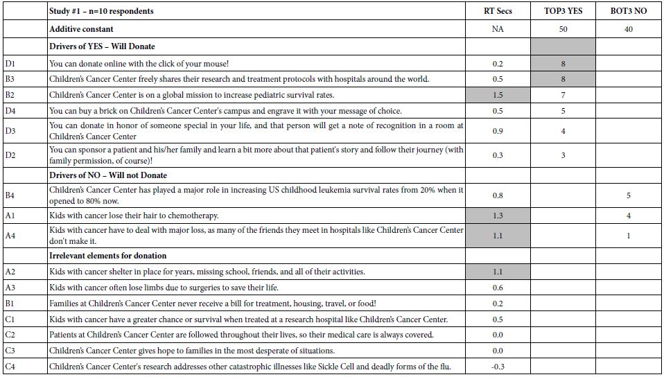
The response time gives a sense of the elements which most engage the respondent. Even with a small base size of 10 respondents, the data from the deconstruction of the ratings into the contribution of the elements gives a sense of the nature of elements that effectively engage. Those elements talk about the children, and survival. The elements may not ‘drive expected donations,’ but they do engage as shown by the long response time (consideration time). Moving on to the ratings, or more specifically the transformed ratings, Table 1 suggests that the additive constant, the proclivity to donate or not to donate ranges between 40 and 50. In the absence of elements which provide specific information, there is no dramatic drive to donate or not to donate, at least for these randomly chosen respondents. What is more important, however, is that among the 16 elements or, the messages, only two reach significance (coefficients of 8 or higher).

You can donate online with the click of your mouse!

Children’s Cancer Center freely shares their research and treatment protocols with hospitals around the world.

The two elements have little in common, suggesting that there is probably no single strong message. It is the nature of researchers to continue looking. These data suggest no ‘magic bullet.’ They do suggest that if there are any ‘magic bullets,’ they may be found in different mind-sets in the population, if such mind-sets can be identified. It is at this point that one can begin to formulate hypotheses about the psychology of donations. The hypothesis emerging here is that ‘painting a graphic word picture’ of the child will engage attention. The science of Mind Genomics has now enriched our thinking about the psychology of donations and generosity, suggesting that graphic design of the recipient is something to consider. The data suggest a further opportunity to understand the nature of the portrait being painted.

Study 2: Identifying the Underlying Structure of What Works for Donating to the Hospital

Study 1 constituted the first foray into the topic, executed with 10 respondents. Although 10 respondents are not often considered to be sufficient to establish results, a base of 10 respondents from one or two focus groups is acceptable when considered to be an exploratory step. Thus, we considered Study 1 to be exploratory, providing information in a disciplined way, but with simply too few respondents.

Here again are the questions from Study 1

Question A: What is it like to be a pediatric cancer patient?

Question B: Why is it important to support Children’s Cancer Center?

Question C: What are the outcomes for children when you donate?

Question D: How do you give your donation?

Based upon the patterns of responses, here are the four revised questions. The key change is Question D, and of course the text of the elements themselves.

Question A: What is it like to be a pediatric cancer patient (why would you want to help)?

Question B: Why is it important to support Children’s Cancer Center?

Question C: What are the outcomes for children when you donate?

Question D: What would inspire you to give?

The second study was conducted with 50 respondents, of which the data from 48 respondents were retained. The remaining two respondents did not provide age or gender, and so their data were eliminated.

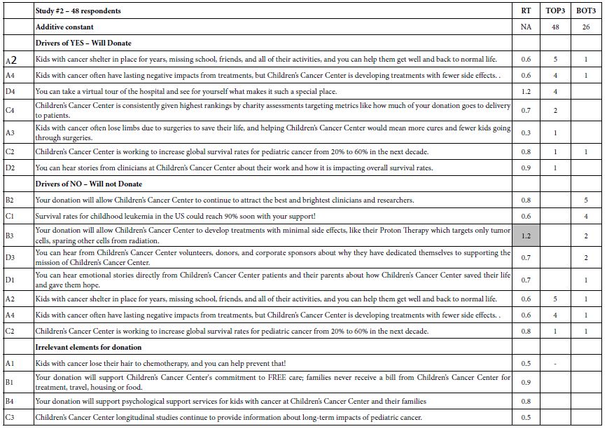
Table 2 shows the same type of data as does Table 1, this time for the new set of respondents, and the new set of elements. Once again, each respondent evaluated a unique set of 24 vignettes, constructed by experimental design, so that the data can be analyzed down to the level of the individual respondent. This strategy, so-called ‘within-subjects design’ ensures that the data can be further deconstructed into subgroups called ‘mind-sets,’ based upon the patterns of the coefficients for each respondent. At first glance, the data reaffirm the previous finding from Study #1 that there are no elements which strongly driving expected donations, when the topic is associated with Children’s Cancer Center. One might consider this a failure when the objective is to discover the so-called ‘magic bullet,’ the message that will work for everyone. The result might be the continued search for this ‘magic bullet’ in successive efforts, only to realize in the end that there is no ‘magic bullet,’ or if there is, no one has any idea about what specifically it is  and how to express it. At the practical level, the effort will be seen to have been wasted. There will be no science of communication about charitable contributions and how people feel. The unsatisfactory conclusion, soon to be discarded is ‘no business results, no contributions to the science of people, no additional knowledge for science of charity communications.’

Table 2: Results from the total panel from Study #2.

table 2

The picture changes, and significant learning for practical application and for foundational knowledge emerges, when one dives more deeply into Mind Genomics and discovers mind-sets. In Mind Genomics, the continuing data suggest the existence of what could be called mind-sets, different patterns of ideas which are interpretable in the form of a ‘story,’ patterns that seem to attach themselves to people. In the world of Mind-Genomics, considering people simply as ‘protoplasm which responds,’ there emerge groups of ideas which separately drive strong responses. People are the carriers of these ideas. People allow these groups of ideas to emerge. A person typically falls into a specific mind-set for a topic and not into the other mind-sets for the same topic. When we look at the data through the lens of mind-sets, using the computational process outlined in Steps 9 and 10 above and doing the computation on the Top3 (positive responses), we emerge with three new-to-the-world mind-sets, shown in Table 3 for Top3 (positive response – likely to donate), and in Table 4 for Bot3 (negative response – not likely to donate).

Table 3: Drivers of positive responses to messages, showing total panel, gender, and the three emergent mind-sets based on clustering using Top3.

table 3

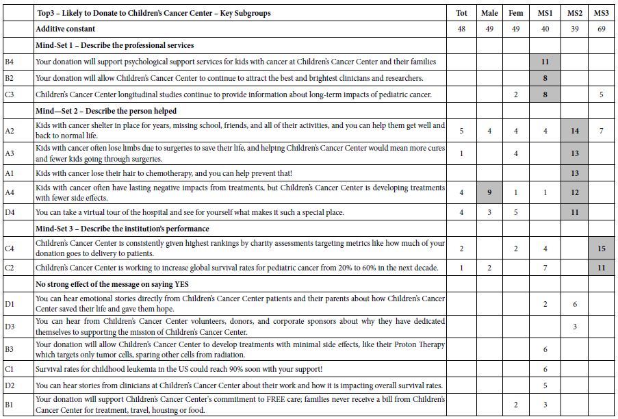
To strengthen the scientific aspect of the results—the learning which is meant to be foundational rather than simply a direction for messaging to raise money—we include gender, as well, comparing the responses of males and females. Table 3 suggests three mind-sets. It is in the mind-sets that the strong elements emerge, elements with coefficients of +8 or higher.

a. There are some positive elements by gender, but no strong performers at all. Both male and female respondents are modestly interested in donating (additive constant=49)

b. Mind-Set 1 – Describe the professional services (modestly interested in donating at a basic level, additive constant=40)

c. Mind-Set 2 – Describe the person helped (modestly interested in donating at a basic level, additive constant=39)

d. Mind-Set 3 – Describe the institution’s performance (strongly interested in donating at a basic level, additive constant=69).

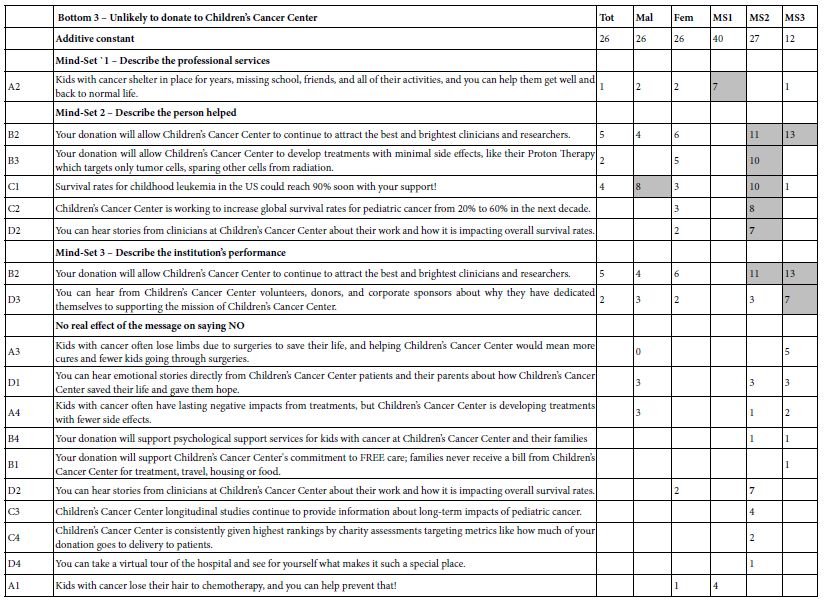
Table 4 shows the messages that should be avoided, the messages driving the response of ‘Not Donate.’ The coefficients emerge from considering only ratings of 1 and 2 as relevant on the 5-point scale, with ratings of 3-5 (neutral, will donate) as not relevant, and coded as 0. The additive constant is far lower for Not Donate than it is for Donate, meaning that people are more inclined to say that they will donate. Several messages to be used by the Center are likely to ‘backfire’, driving donors away. Mind-Set 2 is especially sensitive to the wrong messages.

Table 4: Drivers of negative responses to messages, showing total panel, gender, and the three emergent mind-sets based on clustering using Top3.

table 4

Finding these Respondents in the Population

A continuing topic in Mind Genomics is the value of a ‘next step’ beyond the already-important discovery of mind-sets. Mind-sets themselves provide a way of understanding daily life, through a new focus on the every-day and the way people differ in their typical behaviors. Yet, beyond the scientific contribution of knowledge is the remarkable potential of expanding the value of the learning, moving beyond the respondents tested in the study to the entire world. A simile is the colorimeter used to quantify colors of objects. The science of color can be developed in any location with any material. The real value of the science in terms of the ‘world outside’ is to measure the colors of new objects, not by repeating the study in which the colors were discovered, but rather by measuring the colors of the new objects using a machine in which the science has been already programmed [17-23]. The approach used in Mind Genomics is called the PVI, the personal viewpoint identifier. The objective is to use the data from Table 3 (MS1, MS2, MS3) to create a short questionnaire (six questions), on a simple to-use scale. The questions come from the actual study. The pattern of responses assigns a NEW PERSON to one of the three mind-sets. There are 64 possible patterns, each pattern mapping to one of the three mind-sets. Figure 1 shows the PVI, doing so in two parts. The left part is a short introduction, to introduce the person to the task, and to obtain optional background information. The right part is the actual PVI, including some basic questions about attitudes towards ‘giving’ and the six-question PVI. The results are forwarded to a database and can be sent to the respondents, as well.

fig 1

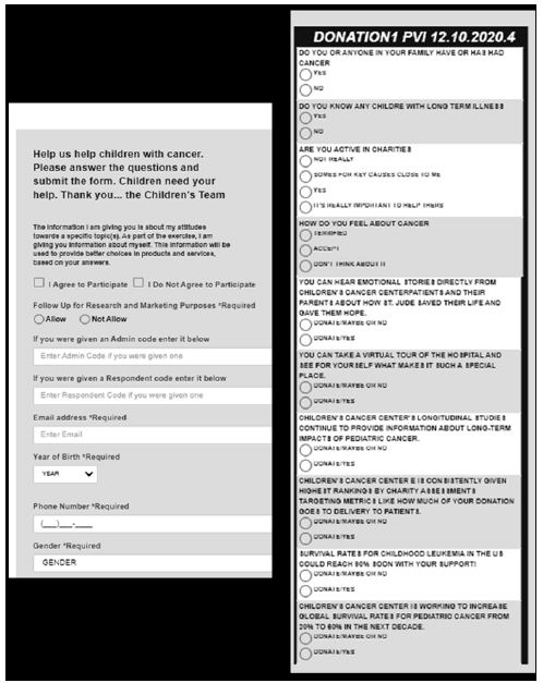
Figure 1: The PVI, personal viewpoint identifier, based upon the second study. The PVI is located at: https://www.pvi360.com/TypingToolPage.aspx?projectid=1261&userid=2018.

Discussion and Conclusion

The empirical results are simple to discover, just by looking at the table of elements and how the elements or messages drive interest in donating. The message used in requesting should be straightforward and focus on how the organization saves and changes lives for the better. The outcome of the organization’s work, and not the process, should be the main message. One should avoid directly focusing on needs and tax breaks, respectively. Although a minority of prospective donors will care about needs or tax advantages, most people say that they will contribute when they are suitably convinced by the cause and mission of the effort and in the vision detailing how their contribution can help. It is at this point that one can begin to formulate hypotheses about the psychology of donations. The hypothesis emerging here is that ‘painting a graphic word picture’ of the child will engage attention. The science of Mind Genomics has now enriched our thinking about the psychology of donations and generosity, suggesting that graphic design of the recipient is something to consider. The data suggest a further opportunity to understand the nature of the portrait being painted. It is not important to point out major ‘learnings’ from the results, learnings which confirm or disconfirm what is known in the literature, or what is hypothesized to be the case for the psychology of donors or the psychology of children with cancer. That information is, of course, important to know for science. What is more important, however, is the ability to have at one’s disposal a tool for small-scale, iterative experimentation: Mind Genomics, a tool which returns rich information even with remarkably small base sizes, such as n=10 or even fewer. In the world of science, Mind Genomics becomes a tool bridging the gap between the idiographic (individual) and the nomothetic (the general world). Just as important, Mind Genomics becomes both a practical tool to increase donations, as well as a tool for the development of systematized knowledge, both for the current generation and for those to come—a ‘wiki of the mind.’ Finally, viewed from the grand proscenium arch of civilization, Mind Genomics provides a record of how people of a certain time, in a specific environment, and faced with known needs, think about topics— a record of inestimable value to philosophy, psychology, history, sociology, anthropology, and economics, just to name a few disciplines where knowledge of the granular is important.

References

  1. Cao X, Jia L (2017) The effects of the facial expression of beneficiaries in charity appeals and psychological involvement on donation intentions: evidence from an online experiment. Nonprofit Management and Leadership 27: 457-473.
  2. Das N, Guha, A, Biswas A, Krishnan B (2016) How product–cause fit and donation quantifier interact in cause-related marketing (CRM) settings: Evidence of the cue congruency effect. Marketing Letters 27: 295-308.
  3. Mejova Y, Garimella VRK, Weber I, Dougal MC (2014) February. Giving is caring: understanding donation behavior through email. In Proceedings of the 17th ACM conference on Computer supported cooperative work & social computing pg: 1297-1307.
  4. Childhood Cancer Survivor Study: An Overview. (2018, September 27). The National Cancer Institute. https://www.cancer.gov/types/childhood-cancers/ccss
  5. Childhood Cancer. (2020, Nov 7). The National Cancer Institute. https://www.cancer.gov/types/childhood-cancers
  6. Alex’s Lemonade (2020) Global Childhood Cancer Facts: By the Numbers. (2020, Dec 7). Alex’s Lemonade. https://bit.ly/3a49Cpl
  7. Connor, K. (2015, May 25). Why childhood cancer research gets shortchanged. Washington Examiner. https://www.washingtonexaminer.com/why-childhood-cancer-research-gets-shortchanged.
  8. Jude’s Children Research Hospital, 2020 Childhood Cancer Facts. (2020, Dec 7). St. Jude Children’s Research Hospital. https://www.stjude.org/treatment/pediatric-oncology/childhood-cancer-facts.html .
  9. Gabay G, Moskowitz HR (2012) The algebra of health concerns: implications of consumer perception of health loss, illness and the breakdown of the health system on anxiety. International Journal of Consumer Studies 36: 635-646.
  10. Galanter E, Moskowitz H, Silcher M (2011) The Price of Grace: Donations, Charities, and the Mind. People, Preferences and Prices: Sequencing the Economic Genome of the Consumer Mind pg:103.
  11. Moskowitz HR, Gofman A (2007) Selling blue elephants: How to make great products that people want before they even know they want them. Pearson Education.
  12. Williams LL, Quave K (2019) Quantitative Anthropology, A workbook. Elsevier.
  13. Gabay G, Moskowitz H, Gere A (2019) September. UNDERSTANDING THE DONATING MIND & OPTIMIZING MESSAGING–PUBLIC HOSPITALS. In 12th Annual Conference of the EuroMed Academy of Business.
  14. Gofman A, Moskowitz H (2010a) Isomorphic permuted experimental designs and their application in conjoint analysis. Journal of Sensory Studies 25: 127-145.
  15. Moskowitz H, Gofman A, I novation Inc (2003) System and method for content optimization. U.S. Patent 6,662,215.
  16. Ramasubbareddy S, Srinivas TAS, Govinda K, Manivannan SS (2020) Comparative Study of Clustering Techniques in Market Segmentation. In Innovations in Computer Science and Engineering, pg: 117-125, Springer, Singapore.
  17. Gofman A, Moskowitz, HR (2010b) Improving customers targeting with short intervention testing. International Journal of Innovation Management, 14: 435-448.
  18. Global Initiative for Childhood Cancer. World Health Organization. (2020, December 7). https://www.who.int/cancer/childhood-cancer/en/
  19. Health Affairs, 2020. https://www.healthaffairs.org/doi/full/10.1377/hlthaff.25.2.541
  20. Importance of CEO involvement in creating a culture of philanthropy in hospitals.
  21. Moskowitz HR, Gofman A, Innovation Inc, (2011). System and method for performing conjoint analysis. U.S. Patent 7,941,335.
  22. Notaro S (2020) https://bit.ly/3b7wBQi.
  23. Social Science Direct (2020) https://www.sciencedirect.com/science/article/abs/pii/S2213076415300051. Use of social media by US Children’s’ hospitals.

Do Pathogenic Chronic Infections Cause Host Senescence?

DOI: 10.31038/TVI.2021122


Aging and senescence are words used as synonyms, and refer to the progressive and deleterious changes that occur in cells, tissues and organs, which alter their functionality [1]. In complex multicellular organisms such as animals, aging begins as soon as embryonic development reaches its maximum stage of differentiation. Aging cannot solely be explained by telomere shortening optics, but rather a combination of factors,including protein assembly and packaging errors, somatic mutations and errors in DNA repair, free radicals, reactive oxygen species, and epigenetic modifications such as hypermethylation [2]. Through molecular control, cells in their maximum state of differentiation stop dividing or reduce their cell division rates. Even tissues of intense proliferation accumulate mutagenic events, whether by environmental factors, by pathogenic infection, or by the events described above that stimulate senescence. Physiologically, our body uses strategies to eliminate senescent cells, damaged cells, or are able to recycle malformed organelles or proteins without the need for cellular elimination. Through autophagy or the removal of senescent cells by the immune system, our body prevents the accumulation of these cells, thus controlling, for example, the growth of tumors3. This is why there is a higher incidence of tumors in the elderly [3].

Through the action of NK cells and CD8+ T cells, the immune system is able to eliminate any cells whose surface protein expression indicates signs of damage and/or malignant transformation. During senescence, there is a significant reduction in the ability of immune cells to fight pathogens, leading to chronic infection [4]. A classic example of senescent cell control and elimination is the red blood cells. Mature red blood cells are anucleated cells whose half-life is approximately 115 days. After this period they become senescent, with the gradual deterioration of their capacity, and they are subsequently eliminated in the spleen. Red blood cells have surface molecules that signal their state of senescence, indicating the right time to eliminate them. The formation of band 3 protein aggregates (one of the most abundant red cell transmembrane proteins), when stabilized by oxidized hemoglobin molecules (hemichromes), are recognized as antigens by autologous IgG antibodies and complement system. With the deposition of a critical density of antibodies and complement molecules, senescent red blood cells are recognized and eliminated [5].

The senescent red blood cells expose phosphatidylserine on the outer portion of their plasma membrane, a sign that indicates that the cell should be phagocytosed. In healthy cells this phospholipid is actively maintained in the cytoplasmic portion of the plasma membrane. Concomitantly, there is down-regulation of the CD47 molecule, a transmembrane protein whose normal expression indicates a non-phagocytic signal. The exposure of phosphatidylserine coupled with the reduction of CD47 expression stimulates phagocytosis and the elimination of these red blood cells [6]. In 2001, Bratosin [7] and colleagues described a process similar to apoptosis occurring in red blood cells, later called erythrosis [8]. Eryptosis has several similarities to apoptosis, regardless of the trigger, induction of an eripotic state usually involves extracellular calcium entry into the cell, caspase and calpain activation, which causes changes in membrane asymmetry, phosphatidylserine exposure and cell shrinkage. and membrane. Erythrosis has been associated with several pathologies, including metabolic syndromes, uremic syndromes, anemias such as sickle cell anemia and thalassemia, and can be triggered by several signs, including osmotic shock and xenobiotics [5].

Infectious processes also induce erythrosis, such as Plasmodium infection that cause malaria [5]. Infection with P. falciparum induces oxidative stress, promoting the opening of calcium channels. Erythrosis also appears to be induced in uninfected red blood cells, both in P. yoelii [9] and P. falciparum infections [10]. That is, chronic infection during malaria induces early red blood cell senescence. Autophagy is a physiological mechanism that allows cells to recognize damaged proteins or organelles and destroy them. In situations of mitochondrial stress, such as the increase of reactive oxygen species, autophagic processes may induce apoptosis cell death [11]. Autophagy also participates in the protection against some intracellular pathogens, although some are able to escape phagolysosome degradation. The relationship between autophagy and senescence is that the latter is characterized precisely by cells resistant to apoptosis and whose autophagic processes do not occur [12].

Like malaria, other chronic infections can also induce host aging. Some bacteria, viruses and protozoa are capable of causing tissue stress leading to molecular and physiological changes in host cells leading to a senescence process. In individuals with cystic fibrosis caused by Pseudomonas aeruginosa, it is believed that the pyocyanin bacterial toxin prevents autophagy. This is due to the increased production of reactive oxygen species, preventing the scaling of the pulmonary epithelium and thus facilitating bacterial colonization [13]. Furthermore, chronic infection with Chlamydia trachomatis, induces increased DNA methylation, and consequently senescence [14].

In infection with Mycobacterium tuberculosis, it is believed that autophagy would function as a protective factor against infection, representing an efficient antimicrobial factor. Although the bacterial toxin ESAT-6 inhibits autophagosome maturation, it is believed that inhibition of autophagy is an activated factor of senescence, so factors that induce autophagosome maturation, such as IFN-gamma, would be inhibitors of senescenia [3]. Coinfection between M. tuberculosis and HIV induces high viremia and functionally altered CD8+ T lymphocytes, which are associated with increased expression of cellular markers associated with this characteristic, as well as the absence of other activation factors such as perforins, granzymes and intracellular IFN-gamma [15].

This state of T lymphocytes is compatible with immunosenescence, which is the aging of the immune system that can be caused by chronic infections, such as HIV, Plasmodium spp., or also by tumors [16]. As with M. tuberculosis infection, Trypanosoma cruzi infection is another example of a chronic infection that induces host senescence related to autophagy blockade [17]. In Chagas disease, we observed lymphopenia and signs of T-cell senescence. In patients infected with T. cruzi, CD8+ and CD4+ T cells display markers of immunosensitivity and show a depleted functional phenotype with decreased production of IFN-gamma and IL-23. Along with evasion of the immune system, T. cruzi can also prevent autophageal intracellular degradation by compromising autophagosome maturation. Autophagy blockade contributes, as the protection of cellular stress, to the activation of senescence [3].

References

  1. Balcombe N, Sinclair A (2001) Ageing: definitions, mechanisms and the magnitude of the problem. Best Pract Res Clin Gastroenterol 15: 835-849. [crossref]
  2. Teixeira INDO, Guariento ME (2010) Biology of aging: theories, mechanisms, and perspectives. Ciênc. Saúde Coletiva 15: 6.
  3. Aguilera MO, Delgui LR, Romano PS, Colombo MI (2018) Chronic Infections: A Possible Scenario for Autophagy and Senescence Cross-Talk. Cells7: 162. [crossref]
  4. Franceschi C, Bonafe M, Valensin S, Olivieri F, De Luca M, et al. (2007) Inflammaging and anti-inflammaging: a systemic perspective on aging asd longevity emerged from studies in humans. Mech Ageing Dev 128: 92-105. [crossref]
  5. Lang F and Qadri SM (2012) Mechanisms and Significance of Eryptosis, the Suicidal Death of Erythrocytes. Blood Purif 33: 125-30. [crossref]
  6. Boulet C, Doering CD, Carvalho TG (2018) Manipulating eryptosis of human red blood cells: a nnovel antimalaraial strategy? Frontiers in Cellular and Infection Microbiology 8: 1-18. [crossref]
  7. Bratosin D, Estaquier J, Petit F, Arnoult D, Quatannens B, et al. (2001) Programmed cell death in mature erythrocytes: a model for investigating death effector pathways operating in the absence of mitochondria. Cell Death Differ 8: 1143-1156. [crossref]
  8. Lang K, Lang P, Bauer C, Duranton C, Wieder T, Huber S, et al. (2005) Mechanisms of suicidal erythrocyte death. CPB 15: 195-202. [crossref]
  9. Totino PRR, Pina RA, De-Oliveira ACAX, Banic DM, Daniel-Ribeiro CT, et al. (2013) Apoptosis of non-parasitised red blood cells in Plasmodium yoelii malaria. Mem Inst Oswaldo Cruz 108: 686-690. [crossref]
  10. Totino PRR, Magalhães AD, Silva LA, Banic DM, Daniel-Ribeiro CT, et al. (2010) Apoptosis of non-parasitized red blood cells in malaria: a putative mechanism involved in the pathogenesis of anaemia. Malar J 9: 350. [crossref]
  11. Dikic I (2007) Proteasomal and Autophagic Degradation Systems. Rev. Biochem 86: 193-224.
  12. Campisi J, D’Adda Di Fagagna F (2007) Cellular senescence: When bad things happen to good cells. Rev. Mol. Cell Biol 8: 729-740. [crossref]
  13. Luciani A, Villella VR, Esposito S, Brunetti-Pierri N, Medina D, et al. (2010) Defective CFTR induces aggresome formation and lung inflammation in cystic fibrosis through ROS-mediated autophagy inhibition. Cell Biol 12: 863-875. [crossref]
  14. Kessler M, Hoffmann K, Fritsche K, Brinkmann V, Mollenkopf H-J, et al. (2019) Chlamydia infection in human organoids increases stemness and promotes age-dependent CpG methylation. Nature Communications 10: 1194. [crossref]
  15. Barathan M, Mohamed R, Vadivelu J, Chang LY, Vignesh R, et al. (2017) CD8+ T cells of chronic HCV-infected patients express multiple negative immune checkpoints following stimulation with HCV peptides. Immunol 313: 1-9. [crossref]
  16. Chou JP, Effros RB (2013) T Cell Replicative Senescence in Human Aging. Current Pharmaceutical Design 19: 1680-1698. [crossref]
  17. Onizuka Y, Takahashi C, Uematsu A, Shinjo S, Seto E, et al. (2017) 1. Inhibition of autolysosome formation in host autophagy by Trypanosoma cruzi Acta Trop 170: 57-62. [crossref]

The Trojan Horse Strategies of Parasites

DOI: 10.31038/TVI.2021121


The Trojan Horse is a legendary figure of a wooden horse used by the Greeks during the Trojan War to invade and destroy the Trojan city. Inside this seemingly harmless horse, supposedly sent as a sign of truce, were Greek warriors who at dusk, when the Trojan defenses were unarmed, took advantage to attack the city. This legendary figure can be used as an excellent analogy for the mechanisms some pathogens have adopted to invade the host and evade detection by the immune system. The ‘Trojan Horse Theory’ in immunology describes the ability of some microorganisms, using cells of the immune system itself as vectors, to escape the immune response.

The cells commonly used by these pathogens are phagocytes, such as neutrophils and macrophages, which are the first cells to reach the site of infection. These cells have microbicidal mechanisms that are able to eliminate the pathogen and aid in the control of infection. These mechanisms depend on the production of cytokines and chemokines, as well as the production of reactive oxygen and interferon species. However some pathogens are able to circumvent or inhibit some of these mechanisms thus allowing their survival, as well as enabling their dissemination to target sites, where they will multiply protected from the action of the immune system [1].

The neutrophil is the first cell that migrates to infected tissue after inoculation of the promastigote form of the protozoan parasites of the genus Leishmania. Leishmania is capable of inhibiting neutrophil proinflammatory cytokine production, such as TNF-α, increasing the production of anti-inflammatory cytokines, such as TGF-β, as well as preventing neutrophil microbicidal activity by negatively regulating IFN-γ. In addition, the parasite is capable of retarding neutrophil apoptosis, which would naturally go into apoptosis 6-10 hours after activation, to up to two days. Leishmania achieves this by interfering with the caspase pathway, preventing the processing of pre-caspase into caspase 3 [2,3].

The infected and apoptotic neutrophil secretes high levels of the chemokine MIP-1b, which attracts macrophages to the infection site. The moment the infected neutrophil becomes apoptotic and releases MIP-1b coincides with the peak migration of macrophages into infected tissue, so in situ macrophages encounter apoptotic neutrophils containing intracellular parasites rather than free Leishmania promastigotes. Since apoptotic cell phagocytosis is an anti-inflammatory signal, macrophage microbicidal functions are not activated, and the parasite survives [3].

The Trojan Horse Theory can also used to explain how some microorganisms can overcome the blood-brain barrier to reach the brain. The blood-brain barrier is composed of endothelial cells lining the vascular and cerebral system and plays an essential role in the maintenance of hemostasis of neurons and glial cells, and blocking access of endogenous or exogenous toxic substances, including microorganisms [4]. However, some pathogens are able to cross this barrier. The first step is the infection of a phagocyte in the periphery. Once internalized, the pathogen can actively manipulate the phagocyte to promote brain migration; alternatively, it can suppress phagocyte activation and consequent sequestration in the source tissue, allowing the infected cell to circulate normally throughout the body. When an infected phagocyte reaches the brain, it adheres to the luminal side of the brain capillaries (with or without activation of BMECs) and crosses the blood-brain barrier between or through endothelial cells. Upon entry into the brain, the pathogen can exit its Trojan horse to infect other neural structures [5]. This model has been elucidated in more detail for HIV6 and other viruses, but other studies indicate similar strategies are utilized by some bacteria, fungi and protozoa, such as Listeria monocytogenes [6-10], Cryptococcus neoformans [11] and Plasmodium spp [12].

The dendritic cell (DC) can also act as a Trojan horse in some infections. During HIV infection, DCs perform two contradictory functions. On the one hand they are essential for building an efficient response against the virus, and are even the target of several studies for the development of HIV vaccines, whilst on the other hand it carries the virus directly to its target cell, the CD4+ T lymphocyte [13]. The CD4 molecule is the HIV-1 receptor, its binding to this receptor and the CCR5 or CXCR4 co-receptors allows the virus to enter the cell and follow its conventional viral cycle, including retrotranscription of its genetic material and integration into the genome. Productive CD infection is a very rare event, less frequent than CD4+ T lymphocyte infection. The type-C lectin receptor, DC-SIGN, which is highly expressed in local DCs.

References

  1. Medzhitov R (2007) Recognition of microorganisms and activation of the immune response. NATURE 449: 18. [crossref]
  2. van Zandbergen G, Klinger M, Muller A, Dannenberg S, Gebert A, (2004) b. Cutting edge: neutrophil granulocyte serves as a vector for Leishmania entry into macrophages. J Immunol 173: 6521-6525. [crossref]
  3. Laskay T, Zandbergen G, Solbach W (2007) Neutrophil granulocytes as host cells and transport vehicles for intracellular pathogens: Apoptosis as infection-promoting factor. Immunobiology 213: 183-191. [crossref]
  4. Daneman R, Prat A (2015) The blood-brain barrier. Cold Spring Harb Perspect Biol 7: a020412. [crossref]
  5. Santiago-Tirado FH, Doering TL (2017) False friends: Phagocytes as Trojan horses in microbial braininfections. PLOS Pathogens 13(12). [crossref]
  6. Kim WK, Corey S, Alvarez X, Williams K (2003) Monocyte/macrophage traffic in HIV and SIVencephalitis. J Leukoc Biol 74: 650-656. [crossref]
  7. Prats N, Briones V, Blanco MM, Altimira J, Ramos JA, et al. (1992) Choroiditis and meningitis in experimental murine infection with Listeria monocytogenes. Eur J Clin Microbiol Infect Dis 11: 744-747. [crossref]
  8. Drevets DA, Bronze MS (2008) Listeria monocytogenes: epidemiology, human disease, and mechanisms of brain invasion. FEMS Immunol Med Microbiol 53: 151-165. [crossref]
  9. Drevets DA, Jelinek TA, Freitag NE (2001) Listeria monocytogenes-infected phagocytes can initiate central nervous system infection in mice. Infect Immun 69: 1344-1350. [crossref]
  10. Join-Lambert OF, Ezine S, Le Monnier A, Jaubert F, Okabe M, et al. (2005) Listeria monocyto- genes-infected bone marrow myeloid cells promote bacterial invasion of the central nervous system. Cell Microbiol 7: 167-180. [crossref]
  11. Srikanta D, Santiago-Tirado FH, Doering TL (2014) Cryptococcus neoformans: historical curiosity to modern pathogen. Yeast 31: 47-60. [crossref]
  12. Wykes MN, Horne-Debets J (2012) Dendritic cells: The Trojan horse of malaria? International Journal for Parasitology 42: 583-587. [crossref]
  13. Martín-Moreno A, Muñoz-Fernández MA (2019) Dendritic Cells, the Double Agent in the War Against HIV-1. Front Immunol 10: 2485. [crossref]