Abstract

The paper deals with the inner mind of the respondent about climate change, using Mind Genomics. Respondents evaluated different combinations of messages about problems and solutions touching on current and future climate change. Respondents rated each combination on a two-dimensional scale regarding believability and workability. The ratings were deconstructed into the linkage between each message and believability vs. workability, respectively. Two mind-sets emerged,Alarmists who focus on the problems that are obvious to climate change, and Investors who focus on a limited number of feasible solutions.These two mind-sets distribute across the population, but can be uncovered through a PVI, personal mind-set identifier.

Introduction

Importance of the Weather and Climate

As of this writing, the concerns keep mounting about climate change, as can be seen in published material, whether the news or academic papers, respectively.As of this writing, the concerns keep mounting about climate change, as can be seen in published material, whether the news or academic papers, respectively.A search during mid-December 2020 reveal 416 million hits for ‘global warming,’ 350 million hits for ‘global cooling’ 886 million his for ‘weather storms’ and 608 million hits for ‘global weather change.’ The academic literature shows the parallel level of interest in weather and its changes. A retrospective of issues about climate change shows the increasing number of ‘hit’ over the past 20 years, as Table 1 shows. These hits suggest that issues regarding climate change are high on the list of people’s concerns.

Table 1a: Number of ‘hits’ on Google Scholar for different aspects of climate change.

Table 1b: The four questions and the four answers to each question.

Beyond Surveys to the Inside of the Mind

The typical news story about climate changes is predicated on storytelling, combining historical overviews, current economic concerns, description of behavior from a social psychology or sociological viewpoint, and often adoom and gloom prediction which demands immediate action in ordertoday to be forestalled.All aspects are correct, in theory.What is missing is a deeper understanding of the inner thinking of a person when confronting the issue of climate change. There are some papers which do deal with the ‘mind’ of the consumer, usually from the point of view of social psychology, rather than experimental psychology [1].

Most conversations about climate change are general, because of the lack of specific knowledge, and the inability of people to deal with the topic in depth. The topic of climate change and the potential upheavals remains important, but people tend to react in an emotional way, often accepting everything or rejecting what sounds reasonable or what does not sound reasonable, respectively. The result is the ongoing lack of specific information, compounding the growth of anxiety, and the increasingly strident rejectionism by those who fail to respond to a believed impending catastrophe. Another result, just as inaction, is a deep, perplexing, often consuming discourse on the problem, written in way which demonstrates scholarship and rhetorical proficiency, but does not lead to insights or answers, rather to well justified polemics [2-6].The study reported here, a Mind Genomics ‘cartography’ delves into the mind of the average person, to determine what specifics of climate change are believable, what solutions are deemed to be workable, and what elements or messages about climate change engage a person’s attention. The objective is to understand the response to the notion of climate change by focusing of reactions to specifics about climate change, specifics presented to the respondent in the form of small combinations of ‘facts’ about climate [7-9].

Researchers studying how people think about climate follow two approaches, the first being the qualitative approach which is a guided, but free-flowing interview or discussion, the second being a structured questionnaire. The traditional qualitative approach requires the respondent to talk in a group about feelings towards specifics, or even talk an in in-depth, 1:1 interview. These are the accepted methods to explore thinking, so-called focus groups and in-depth interviews. Traditional discussion puts stress on the respondentto recall and state, or, in the language of the experimental psychologist, to produce and to recite. In contrast, the traditional survey presents the respondent with a topic, and asks a variety of questions, to which the respondent selects the appropriate answer, either by choice, or by providing the information.All in all, conventional research gives a sense of the idea, but from the outside in. Reading a book by research can provide extensive information from the outside. Some information from the inside can be obtained from comments by individuals about their feelings.Yet it will be… clearly from the outside, rather than a sense of peering out from the inside of the mind. The qualitative methods may reach into the mind somewhat more deeply because the respondent is asked to talk about a topic and must ‘produce’ information from inside. Both the qualitative and the quantitative methods produce valuable information, but information of a general nature. The insights which may emerge from the qualitative and quantitative methods have a sense of emerging from the ‘outside-in.’ That is, there is insight, but there is not the depth of specific material relevant to the topic, since the qualitative information is in the form of diluted ideas, ideas diluted in a discussion, whereas the quantitative information is structured description with a sense of deep specificity.

The Contribution of Mind Genomics

Mind Genomics is an emerging science, with origins in experimental psychology, consumer research, and statistics.The foundational notion of Mind Genomics is that we can uncover the ways that people make decisions about every-day topics using simple experiments, where people respond to combinations of messages abut the different aspects of the topic. These combinations, created by experimental design, present information to the respondent in a rapid fashion, requiring the respondent to make a quick judgment. The mixture of different messages in a hard-to-disentangle fashion, using experimental design, makes it both impossible to ‘game’ the system, and straightforward to identify which pieces of information drive the judgment.Furthermore, one can discover mind-sets of individuals quite easily, groups of people with similar pattern of what they deem to be important. The approach here, Mind Genomics, makes the respondents job easier, to recognize and react. The messages are shown to the respondent’s job easier, the respondents evaluate the combination, and the analysis identifies which messages are critical, viz, which messages about weather change are important. Mind Genomics approaches the problem by combining messages about a topic, messages which are specific. Thus, Mind Genomics combines the richness of ideas obtained from qualitative research with the statistical rigor of quantitative research found in surveys. Beyond that combination, Mind Genomics is grounded in the world of experiment, allowing the researcher to easily understand the linkage between the qualitatively, rich, nuanced information, presented in the experiment, and the reaction of the respondent, doing so in a manner which cannot be ‘gamed’ by the respondent, in a manner which reveals both cognitive responses (agree/disagree) and non-cognitive response (engagement with the information as measured by response time.)

Mind Genomics follows a straightforward path to understand the way people think about the everyday. Mind Genomics is fast (hours), inexpensive, iterative, and data-intensive, allowing for rapid, up-front analysis and deeper post-study analysis.Mind Genomics has been crafted with the vision of a system which would allow anyone to understand the mind of people, even without technical training. The grand vision of Mind Genomics is to create a science of the mind, a science available to everyone in the world, easy-to-do, a science which creates a ‘wiki of the mind’, a living database of how people think about all sorts of topics.

Doing a Simple Cartography – The Steps

Step 1 – Create the Raw Materials; Topic, Four Questions, Four Answers to Each Question

The cartography process begins with the selection of a topic, here the mind of people with respect to climate change. The topic is only a tool by which to focus the researcher’s mind on the bigger areas.

Following the selection of the topic, the researcher is requested to think of four questions which are relevant to the topic. The creation of these questions may sound straightforward, but it is here that the respondent must exercise create and critical thinking (got rid of word ‘some’), to identify a sequence of questions which ‘tell a story.’ The reality is that it takes about 2-3 small experiments, the cartographies,before the researcher ‘gets it,’ but once the researcher understands how to craft the questions relative to the topic, the researcher’s critical faculty and thinking patterns have forever changed. The process endows the world of research with a new, powerful, simultaneous analytic-synthetic ways to think about a topic, and to solve a problem.Once the four questions are decided upon, the researcher’s next task is to come up with four answers. The perennial issue now arises regarding ‘how do I know I have the right or correct answers?’ The simple answer is one does not. One simply does the experiment, finds out ‘what works,’ and proceeds with the next step of stimuli.After two, three, four, even five or six iterations, each taking 90 minutes, it is likely that one has learned what works and what does not. The iteration consists of eliminating ideas or directions which do not work, trying more of the type of ideas which do work, as well as other exploring other but related directions with other types of ideas.

It is important to emphasize the radically different thinking behind Mind Genomics, which is meant to be fast and iterative, and not merely to rubber stamp or confirm one’s thinking. Speed and iteration lead to a wider form of knowledge, a sense of the boundaries of a topic. In contrast, the more conventional and focused thinking lead to rejection or confirmation, but little real learning.

Step 2 – Combine the Elements into Small Vignettes that will be Evaluatedby the Respondents

The typical approach to evaluation would be to present each of the elements in Table 2 to the respondent, one element at a time, instructing the respondent to rate the element alone, using a scale.Although the approach of isolate and measure is appropriate in science, the approach carries with it the potential of misleading results, based upon the desire of most respondents to give the ‘right answer.’

Mind Genomics works according to an entirely different principle. Mind Genomics presents the answers or elements in what appear to be random combinations, but nothing could be further from the truth. The combinations are well designed, presenting different types of information. It will be the rating of the combination, and then the deconstruction of that rating into the contributions of the 16 individual elements which reveal the mind of the respondent.The experimental design simply ensures that the elements are thrown together in a known but apparently haphazard way, forcing the respondent to rely on intuitive or ‘gut responses,’ the type judgment which governs most of everyday life. Nobel Laureate Daniel Kahnemancalls this ‘System 1’ Thinking, the automatic evaluation of information in an almost subconscious but consistent and practical manner [10].

The underlying experimental design used by Mind Genomics requires each respondent to evaluate 24 different vignettes, or combinations, with a vignette comprising 2-4 elements. Only one element or answer to a question can appear in a single vignette, ensuring that a vignette does not present elements which directly contradict each other, viz., by comprising two elements from the question or silo, presenting two alternative and contradictory answers to the question. The experimental design might be considered as a form of advanced bookkeeping[11].

Many researchers feel strongly that every vignette must have exactly one element or answer from each question.Their point of view is that otherwise the vignettes are not ‘balanced’, viz., some vignettes have more information, some vignettes have less information. Their point of view is acceptable, but by having incomplete vignettes, the underlying statistics, OLS (ordinary least-squares) regression cannotestimate absolute values for coefficients. By forcing each vignette to comprise exactly one element or answer from each question, the OLS regression will not work because the system is ‘multi-collinear.’The coefficients can only be estimated in a relative sense, and not comparable across questions for the study, nor comparable across studies in the same topic, and of course not comparable for different topics.That lack of comparability defeats the ultimate vision of Mind Genomics, viz., to create a ‘wiki of the mind.’A further point regarding the underlying experimental design is that Mind Genomics explores a great deal of the design space, rather than testing the same 24 vignettes with each respondent.Covering the design space means giving up precision obtained by reducing variability through averaging, the strategy followed by most researchers who replicate or repeat the study dozens of times, with the vignettes in different orders, but nonetheless with the same vignettes. The underlying rationale is to average out the noise, albeit at the expense of testing a limited number of vignettes again and again.

Step 3 – Select an Introduction to the Topic and a Rating Scale

The introduction to the topic appears below. The introduction is minimal, setting up as few expectations as possible. It will the job of the elements to convey the information.

Please read the sentences as a single idea about our climate. Please tell us how you feel.

1) No way.

2) Don’t believe, and this won’t work.

3) Believe, but this won’t work.

4) Don’t really believe, but this will work.

5) I believe, and this will work.

The scale for this study is anchored at all five points, rather than at the lowest and at the highest point.The scale deals with both belief in that which iswritten, and belief that the strategy will work.The respondent is required to select one scale point out of the five for each vignette, respectively. The scale allows the researcher to capture both belief in the facts and belief in the solutions.

Step 4 – Invite Respondents to Participate

The respondents are invited to participate by an email. The respondents are member of Luc.id, an aggregator of online panels, with over 20 million panelists. Luc.id, located in Louisiana, in the United States, allows the researcher to tailor the specifications of the respondents. No specifics other than being US residentswere imposed on the panel. The respondents began with a short self-profiling classification questionnaire, regarding age and gender, as well as the answer to the question below:

How involved are you in thinking about the future?

1=Worried about my personal situation with my family

2=Worried about business stability

3=Worried about climate and ecological stability

4=Worried about government stability.

The respondent then proceeded to rate the 24 unique combinations from the permuted experimental design, with the typical time for each vignette lasting about 5-6 seconds, including the actual appearance time, and the wait time before the next appearance[12].The actual experiment thus lasted 2-3 minutes.

Step 6 – Acquire the Ratings and Transform the Data in Preparation for Model

In the typical project the focus of interest is on the responses to the specific test stimuli, whether there be a limited number of test vignettes (viz., not systematically permuted, but rather fixed), or answers to a fixed set of questions.The order of the stimuli or the test questions might be varied but there is a fixed, limited number. With Mind Genomics the focus will be on the contribution of the elements to the responses.Typically, the responses are transformed from a scale of magnitude (e.g., 1-5, not interested to interested), so that the data are binary (viz., 1-3 transformed to 100 to show that the respondents are not interested; 4-5 transformed to 0 to show that the respondent is interested.

As noted above, there are two scales intertwined, a belief in the proposition, and a belief that the action proposed will work. The two scales generate two new binary variables, rather than one binary variable:

Believe:Ratings of 1,2, 4 converted to 0 (do not believe the statements), ratings of 3,5 converted to 100 (believe the statements

Work (Efficacious) Ratings of 1,2,3 converted to 0 (do not believe the solution will work), ratings 4,5 converted to 100 (believe the proposed solution will work).

In these rapid evaluations we do not expect the respondent to stop and think. Rather, it turns out that ‘Believe’ is simply ‘’does it sound true?’ and Work” is simply ‘does it seem to propel people to solve the problem?Both of these are emotional responses. The end-product is a matrix of 24 rows for each respondent, one row for each vignette tested by that respondent. The matrix comprises 16 columns, one column for each of the 16 elements. The cell for a particular row (vignette) and for a particular column (element) is either 0 (element absent from that vignette) or 1 (element present in that vignette). The last four columns of the matrix are the rating (1-5), the response time (in seconds, to the nearest 10^th of a second), and the two new binary values for the scales ‘Believe’ and ‘Work’ respectively (0 for not believe or not work, 100 for believe or work, depending upon the rating, plus a small random number < 10^-5).

Step 7 – Create Two Models (Equations) for Each Respondent, a Model for Believe, and a Model for Work, and then Cluster the Respondents Twice, First for the Individual ‘Believe’ Models, Second for the Individual ‘Work’ Models

The experimental design underlying the creation of the 24 vignettes for each respondent allows us to create an equation at the respondent level for Believe (Binary) = k₀ + k₁(A1) + k₂(A2) …. + k₁₆(D4).The dependent variable is either 0 or 100, depending upon the value of the specific rating in Step 6.The small random number added to each binary transformed number ensures that there is variation in the dependent variable.

1. Believe Models. For the variable Believe, applying OLS regression generates the 16 coefficients (k₁ – k₁₆) and the additive constant, for each of the 55 respondents. A clustering algorithm (k-means clustering, Distance = (1 – Pearson Correlation)) divides the respondents into two groups. We selected the two groups (called mind-sets) because the meanings of the two groups were clear. Each respondent was then assigned to one of the two emergent groups, viz., mind-sets,based on the respondent’s coefficients for Believe as a dependent variable[13].
2. Work Models. A totally separate analysis was done, following the same process, but this time using the transformed variable ‘Work’.The respondents were then assigned to one of the two newly developedmind-sets, based only on the coefficient for work.

As a rule of thumb, one can extract many different sets of complementary clusters (mind-sets), but a good practice is to keep the number of such selected sets to a minimum, the minimum based upon the interpretability of the mind-sets. In the interests of parsimony, one should stop as soon as the mind-sets make clear sense.

Step 8 – CreateGroup Equations; Three Models or Equations, One for Believe, One for Work, One for Response Time

Create these sets of three models each for Total Panel, Male, Female, Younger (age 18-39), Older (age 40+), and the mind-sets.Theequations are similar in format, but not identical:

Believe = k₀ + k₁(A1) + k₂(A2) … k₁₆(D4)

Work = k₀ + k₁(A1) + k₂(A2) … k₁₆(D4)

Response Time=k₁(A1) + k₂(A2) … k₁₆(D4)

For the mind-sets,create two models only.

Mind-Set based on ‘believe’:

Believe = k₀ + k₁(A1) + k₂(A2) … k₁₆(D4)

Response Time= k₁(A1) + k₂(A2) … k₁₆(D4)

Mind-set based on ‘work’

Work =k₀ + k₁(A1) + k₂(A2) … k₁₆(D4))

Response Time =k₁(A1) + k₂(A2) … k₁₆(D4).

Results

External Analysis

The external analysis looks at the ratings, independent of the nature of the vignettes, either structure or composition of the vignette in terms of specific elements. We focus here on a topic which is deeply emotion to some. The first analysis that we will focuses on the stability of the data for this deeply emotional topic. As noted above, the Mind Genomics process requires the respondent to evaluate a unique set of 24 vignettes. Are the ratings stable over time or is there so much random variability that by the time the respondent has completed the study the respondent is not paying any more attention, and simply pressing the rating button?We cannot plot the rating of the same vignette across the different positions for the same reason that each respondent tested a totally unique set of combinations. We can track the average rating, the average response time, and then the standard errors of both, across the 24 positions. If the respondent somehow stops paying attention, then the rating should show less variation over time.

Figure 1 shows the averages and standard errors for the two measures, the ratings actively assigned by the respondent, and the response time, not directly a product of the respondent’s ‘judgment,’ but rather a measure of the time taken to respond. The abscissa shows the order in the test, from 1 to 24, and the ordinate shows the statistic.The data show that the response time is longer for the first few vignettes (viz., test order 1-3), but then stabilizes.The data further show that for the most part, the ratings themselves are stable, although there are effects at the start and at the end. Figure 1 suggests remarkable stability, a stability that has been observed for almost all Mind Genomics studies, when the respondents are members of an on-line panel, and remunerated by the panel provided for their participation.

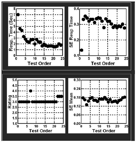
Figure 1: The relation between test order (abscissa) and key measures. The top panel shows the analysis of the response times (mean RT on left, standard error of the mean on the right).The bottom panel shows the analysis of theratings (mean rating on the left, standard error of the mean on the right).

The second external analysis shows the distribution of ratings by key subgroups across all of the vignettes evaluated by each key subgroup. For each key subgroup (rows), Table 2 shows the distribution of the five scale points (A), distribution of the two scale points (3,5) points which reflect belief (3,5) distribution of the two scale points (4,5) reflecting positive feeling that the idea ‘works’ The patterns of ratings suggest that a little fewer than half the responses are believe or work. However, we do not know the specific details about which types of messages drive these positive responses. We need a different level of inquiry, an internal analysis into what patterns of elements drive the responses.

Table 2: Distribution of ratings on Net Believe Yes, and Net Work YES five-point scale, by key groups, and by key clusters of scale points.

Internal Analysis – What Specific Elements Drive or Link with ‘Believe’ and ‘Work’ Respectively?

Up to now we have considered only the surface aspect of the data, namely the reliability of the data across test order (Figure 1), and the distribution of the ratings by key subgroup (Table 2). There is no sense of the inner mind of the respondent, about what elements link with believability of the facts, with agreement that the solution will work, or how deeply the respondent engages in the processing of the message, as suggested by response time. The deeper knowledge comes from OLS (ordinary least squares) regression analysis, which relates the presence/absence of the 16 messages to the ratings, as explicated in Step 8 above.

Table 3 shows the first table of results, the elements which drive ‘believability.’ Recall from the methods section that the 5-point scale had two points with the respondent ‘believing,’ and that these ratings (3,5) generated a transformed value of 100 for the scale of ‘believe’, whereas the other three rating points (1,2,4) were converted to 0.The self-profiling classification also provides the means to assign a respondent based upon what the respondent said was most concerning, worry about self (family, government), worry about other/outside (business, climate).Table 3 shows the additive constant, and the coefficients for each group. Only the Total Panel shows coefficients which are 0 or negative. The other groups show only coefficients which are positive. Furthermore, the table is sorted by the magnitude of the coefficient for the Total Panel.In this way, one need only focus on those elements which drive ‘belief’, viz., elements which demonstrate a positive coefficient. Elements which have a 0 negative coefficient are those which have no impact on believability. They may even militate against believability. Our focus is strictly what drives a person to say ‘I believe what I am reading.’

Table 3: Elements which drive ‘belief ’. Only positive coefficients are shown. Strong performing elements are shown in shaded cells.

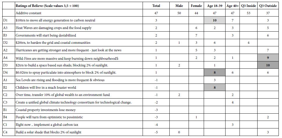
We begin with the additive constant across all of the key groups in Table 3. The additive constants tell us the likelihood that a person will rate a vignette as ‘I believe it’ in the absence of elements. The additive constant is a purely estimated parameter, the ‘intercept’ in the language of statistics. All vignettes comprised 2-4 elements by the underlying experimental design. Nonetheless, the additive constant provides a good sense of basic proclivity to believe in the absence of elements. The additive constants hover between 40 and 50 with two small exceptions of 37 and 53. The additive constant tells us that the respondent is prepared to believe, but only somewhat. In operational terms, an additive constant of 45, for example, means that out of the next 100 ratings for vignettes, 45 will be ratings corresponding to ‘believe,’ viz., selection of rating points 3 or 5, respectively.The story of what makes a person believe lies in the meaning of the elements. Elements whose coefficient value is +8 or higher are strongly ‘significant’ in the world of inferential statistics, based upon the ‘T test’ versus a coefficient with value 0.There are only a few of these elements which drive strong belief.

The most noteworthy finding is that respondents in Q3 Inside (worried about issues close to them) start out with a high propensity to believe (additive constant = 53), but then show no differentiations among the elements. They do not believe anything. In contrast, respondents who say they worry about issues outside of them start with low belief (additive constant = 53), but there are a several of elements which strongly drive their belief (e.g., A4:Wild-Firesare more massive and keep burning down neighborhoods.)They are critical, but willing to believe in what they see, and in what is promised to them.  Table 4 shows the second table of results, elements which drive ‘work’. These elements generate positive coefficients when the ratings 4 or 5 were transformed to 100, and the remaining ratings (1,2,3) were transformed to 0. Only some elements give a sense of a solution, even If not directly a solution.The additive constants showdifferences in magnitude for complementary groups. Since the scale is ‘work’ vs. ‘not work’, the additive constant is the basic belief that a solution will work. The additive constant is higher for males than for females (52 vs. 36), higher younger vs. older (50 v 35), and higher for those who worry about themselves versus those who were about others (49 vs. 36).

Table 4: Elements which drive ‘work’. Only positive coefficients are shown. Strong performing elements are shown in shaded cells.

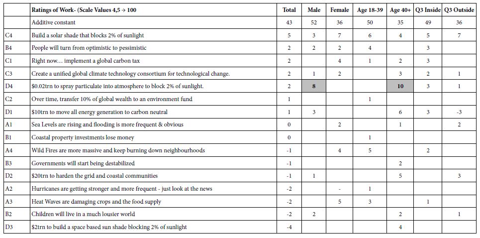
The key finding for ‘work’ is that there some positives on two strong ones. The respondents are not optimistic. There is only one element which is dramatic, however, D4, the plan to spray particulates into the atmosphere to block 2% of the sunlight. This element or plan performs strongly among males, and among the older respondents, 40 years and older, although in the range of studies conducted previously, coefficients of 8-10 are statistically significant but not dramatic, especially when they belong to only one element.  Our third group model concerns the response time associated with each element. The Mind Genomics program measured the total time between the presentation of the vignette and the response to the vignette. Response times of 8 seconds or longer were truncated to the value 8. OLS regression was applied to the data of the self-defined subgroups. The form of the equation for OLS regression was: Response Time = k₁(A1) + k₂(A2) … k₁₆₍D4). The key difference moving from binary rating to response time is the removal of the additive constant. The rationale is that we want to see the number of seconds ascribed to each element, for each group. The longer response times mean that the element is more engaging. Table 5 shows the response times for the total panel, the genders, ages, and the two groups defined by what they say worries them.Table 3 shows only those time coefficients of 1.1 second or more, response times or engagement times that are deemed to be relevant and capture the attention.The strongly engaging elements are shown in the shaded cells.

Table 5: Response times of 1.1second or longer for each element by key self-defined subgroups.

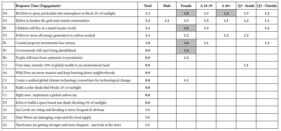
Table 5 suggests that the description of building something can engage all groups

$10trn to move all energy generation to carbon neutral

$20trn to harden the grid and coastal communities

Women alone are strongly engaged when a clear picture is painted, a picture at the personal level:

Coastal property investments lose money

Children will live in a much lousier world

Governments will start being destabilized.

One of the key features of Mind Genomics is its proposal that in every aspect of daily living people vary r in the way they respond to information. These different ways emerge from studies of granular behavior or attitudes, as well as from studies of macro-behavior or attitudes. Traditional segment-seeking research looks for mindsets in the population, trying to find them by knowing their geodemographics.  Both the traditional way of segmentation and the traditional efforts to find these segments in the population end up being rather blunt instruments. The traditional segmentation begins at a high level, encompassing a wide variety of different issues pertaining to the climate, the future, and so forth. The likelihood is minimal of finding the mind-sets with the clear granularity of these mind-sets is low, simply because in the larger scale studies there is no room for the granular, as there is in Mind Genomics, such as this study which deals with 16 elements of stability and destabilization.

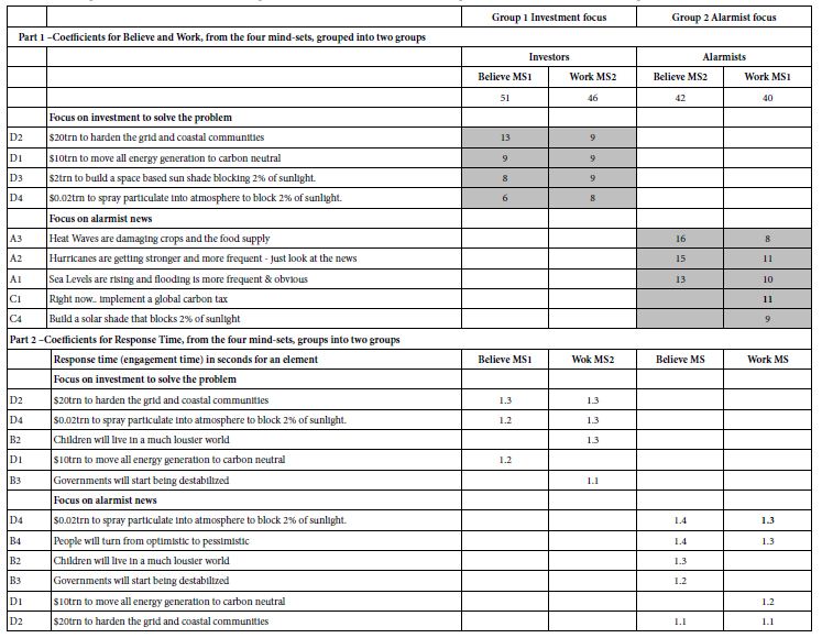
Mind Genomics uses a simple k-means clustering divide individuals based upon the pattern of coefficients. The experimental design used in permuted form for each respondent allows the researcher to apply OLS regression to the binary-transformed data of each respondent.The k-means clustering was applied separately to the 55 models for Believe, and separately once again to the 55 models for Work.Both clustering programs came out with similar patterns, two mind-sets for each. The pattern suggested one be called ‘Investment focus’ and the other be called alarmist focus. The strongest performing elements from this study come from the mind-sets, classifying the respondent by the way the respondent ‘thinks’ about the topic, rather than how the respondent ‘classifies’ herself or himself, whether gender, age, or even self-chosen topic of major concern. The mind-sets are named for the strongest performing element. Group 1 (Believed MS1, Work MS4) show elementswhich suggest an ‘investment focus’.Group 2 (Believe MS2, Work MS3) shows elements which suggest an alarmist focus.

Table 6 shows the strong performing elements for the four mind-sets, as well as the most engaging elements for the mind-sets. The reader can get a quick sense of the nature of the mind-sets, both in terms of what they think(coefficients for Believe and for Work, respectively), as well as what occupies their attention and engages them (Response Time) [14].

Table 6: Strong performing coefficients for the two groups of emergent mind-sets after clustering on responses (Part1), and after clustering on response time, viz., engagement (Part 2).

The mind-sets emerging from Mind Genomics studies do not distribute in the simple fashion that one might expect, based upon today’s culture of Big Data. That is, just knowing WHO a person is does not tell us how a person THINKS. The reality is that there are no simple cross-tabulations or even more complex tabulations which directly assign a person to a mind-set.Topics such as the environment, for example, may have dozens of different facets. Knowing the mind of a person regarding one facet, one specific topic, does not necessarily tell us about the mind of that same person with respect to a different, but related facet.Table 7 gives a sense of the complexity of the distribution, and the probable difficulty of finding these mind-sets in the population based upon simple classifications of WHO is a person is.

Table 7: Distribution of key mind-sets (Investors, Alarmists).

During the past four years authors Gere and Moskowitz have developed a tool to assign new people to the mind-sets. The tool, called the PVI, the personal viewpoint identifier, uses the summary data from the different mind-sets, perturbing these summary data with noise (random variability), and creating a decision tree based upon a Monte Carlo simulation. The decade PVI allows for 64 patterns of responses of six questions answered on a 2-point. The Monte simulation combined with the decision tree returns with a system to identify mind-set member in15-20 seconds.Figure 2 shows a screen shot of the PVI for this study, comprising the introduction, the additional background information stored for the respondent (option), and the six questions, patterns of answers to which assign the respondent immediately to the of the two mind-sets.

Figure 2: The PVI for the study.

Discussion and Conclusion

The study described here has been presented in the spirit of an exploration, a cartography, a way to understand a problem without having to invoke the ritual of hypothesis. In most study of the everyday life the reality is that the focus should be on what is happening, not on presenting an hypothesis simply for the sake of conforming to a scientific approach which is many cases is simply not appropriate.The issue of climate change is an important one, as a perusalof the news of the day will reveal just about any day. The issues about the weather, climate change, and the very changes in ‘mother earth’ are real, political, scientific, and challenge all people. Mind Genomics does not deal with the science of weather, but rather the mind of the individual, doing so by experiments in communication.It is through these experiments, simple to do, easy to interpret, that we begin to understand the nature of people, an understanding which should not, however, surprise.The notion of investors and alarmists makes intuitive sense. These are not the only mind-sets, but they emerge clearly from one limited experiment, one limited cartography.One could only imagine the depth of understanding of people as they confront the changes in the weather and indeed in ‘mother earth.’ Mind Genomics will not solve those problems, but Mind Genomics will allow the problems to be discussed in a way sensitive to the predispositions of the listener, whether in this case the listener be a person interested in investment to solve the problem or the person be interested in the hue and the cry of the alarmist. Both are valid ways of listening, and for effective communication the messages directed towards each should be tailored to the predisposition of the listener’s mind. Thus, a Mind Genomics approach to the problem presents both understanding and suggestion for actionable solution, or at least the messages surrounding that actionable solution [2,15-19].

As a final note this paper introduces a novel way to understand the respondent’s mind on two dimensions, not just one. The typical Likert Scale presents the respondent with a set of graded choices, from none to a low, disagree to agree, and so forth. The Likert Scale for the typical study is uni-dimensional. Yet, there are often several response dimensions of interest.This study features two response dimensions, belief in the message, and belief that the solution will work.These response dimensions may or may not be intertwined.Other examples might be belief vs. action (would buy).By using a response scale comprising two dimensions, rather than one, it becomes possible to more profoundly understand the way a person thinks, considering the data from two aspects. The first is the message presented, the stimulus. The second is the decisions of the respondent, to select none, one, or both responses, belief in the problem and/or, belief that the solution will work

Acknowledgement

Attila Gere thanks the support of Premium Postdoctoral Research Program.

References

1. Tobler C, Visschers VH, Siegrist M (2012) Addressing climate change: Determinants of consumers’ willingness to act and to support policy measures. Journal of Environmental Psychology 32: 197-207.
2. Creutzig F, Fernandez B, Haberl H, Khosla R, Mulugetta Y,et al (2016) Beyond technology: demand-side solutions for climate change mitigation. Annual Review of Environment and Resources 41: 173-198.
3. Lidskog R, Berg M, Gustafsson KM, Löfmarck E (2020) Cold Science Meets Hot Weather: Environmental Threats, Emotional Messages and Scientific Storytelling. Media and Communication 1: 118-128.
4. Nyilasy G, Reid LN (2007) The academician–practitioner gap in advertising. International Journal of Advertising 26: 425-445.
5. Reyes A (2011) Strategies of legitimization in political discourse: From words to actions. Discourse & Society 22: 781-807.
6. Taleb NN (2007) The black swan: The impact of the highly improbable, Random house, Vol:2.
7. Moskowitz HR (2012) ‘Mind genomics’: Theexperimental, inductive science of the ordinary, and its application to aspects of food and feeding. Physiology & Behavior 107: 606-613.
8. Moskowitz HR, Gofman A, Beckley J, Ashman H (2006) Founding a new science: Mind Genomics. Journal of Sensory Studies 21: 266-307.
9. Moskowitz HR, Gofman A (2007) Selling blue elephants: How to make great products that people want before they even know they want them. Pearson Education.
10. Kahneman D (2011) Thinking, fast and slow. Macmillan.
11. Box GE, Hunter WH, Hunter S (1978) Statistics for Experimenters, New York: John Wiley Vol: 664.
12. Gofman A, Moskowitz H (2010) Isomorphic permuted experimental designs and their application in conjoint analysis. Journal of Sensory Studies 25: 127-145.
13. Jain AK, Dubes RC (1988) Algorithms for Clustering Data. Prentice-Hall, Inc.
14. Schweickert R (1999) Response time distributions: Some simple effects of factors selectively influencing mental processes. Psychonomic Bulletin & Review 6: 269-288.
15. Acosta Lilibeth A, Nelson H Enano Jr, Damasa B Magcale-Macandog, Kathreena G Engay, Maria Noriza Q Herrera, et al. (2013) How sustainable is bioenergy production in the Philippines? A conjoint analysis of knowledge and opinions of people with different typologies. Applied Energy 102: 241-253.
16. Lomborg B (2010) Smart solutions to climate change: Comparing costs and benefits. Cambridge University Press.
17. Nerlich B, Koteyko N, Brown B (2010) Theory and language of climate change communication. Wiley Interdisciplinary Reviews: Climate Change 1: 97-110.
18. Tol RS (2009) The economic effects of climate change. Journal of Economic Perspectives 23: 29-51.
19. Warren R (2011) The role of interactions in a world implementing adaptation and mitigation solutions to climate change. Philosophical Transactions of the Royal Society A: Mathematical, Physical and Engineering Sciences 369: 217-241.

References

1. Guan WJ, Ni ZY, Hu Y, Liang WH, Ou CQ, et al. (2020) Clinical characteristics of coronavirus disease 2019 in China. N Engl J Med.
2. Lingzhong Meng, Haibo Qiu, Li Wan, Yuhang Ai, Zhanggang Xue, et al. (2020) Intubation and Ventilation amid the COVID-19 Outbreak: Wuhan’s Experience. Anesthesiology 132: 1317-1332. [crossref]
3. Huang C, Wang Y, Li X, Ren L, Zhao J, et al. (2020) Clinical features of patients infected with 2019 novel coronavirus in Wuhan, China. Lancet 395: 497-506.
4. Qin Liu, Rongshuai wang, Guoqiang Qu, Yunyun wang, Pan Liu, et al. (2020) Gross Observation Report on the Autopsy of a nCov-2019 Pneumonia Death. Journal of Forensic Medicine (Chinese) 36: 21-23. [crossref]
5. Hsu CF, Cheng JS, Lin WC, Cheng KS, Lin SH, et al. (2016) Electrical impedance tomography monitoring in acute respiratory distress syndrome patients with mechanical ventilation during prolonged positive end-expiratory pressure adjustments [J]. J Formos Med Assoc 115: 195-202. [crossref]
6. Staub LJ, Mazzali Biscaro RR, Kaszubowski E, Maurici R (2019) Lung ultrasound for the emergency diagnosis of pneumonia, acute heart failure, and exacerbations of chronic obstructive pulmonary disease / asthma in adults: a systematic review and meta-analysis. J Emerg Med 56: 53-69. [crossref]
7. Heines SJH, Strauch U, Van de Poll MCG, Paul MHJR, Dennis CJJB (2018) Clinical implementation of electric impedance tomography in the treatment of ARDS: a single centre experience [J]. J Clin Monit Comput. [crossref]
8. Rouby JJ, Arbelot C, Gao YZ, Zhang M, Lv J, et al. (2018) APECHO Study Group. Training for lung ultrasound score measurement in critically ill patients. Am J Respir Crit Care Med 198: 398-401. [crossref]
9. Lichtenstein DA (2015) BLUE-protocol and FALLS-protocol: two applications of lung ultrasound in the critically ill. Chest 147: 1659-1670.
10. Chavez MA, Shams N, Ellington LE, Naithani N, Gilman RH, et al. (2014) Lung ultrasound for the diagnosis of pneumonia in adults: a systematic review and meta-analysis. Respir Res 15: 50. [crossref]
11. Long L, Zhao HT, Zhang ZY, Wang GY, Zhao HL (2017) Lung ultrasound for the diagnosis of pneumonia in adults: a meta-analysis. Medicine (Baltimore) 96: e5713. [crossref]
Thinking Climate – A Mind Genomics Cartography
1. Hsu, Gerald C. eclaireMD Foundation, USA (2020) Analyzing CGM sensor glucoses at 5-minute intervals using GH-Method: math-physical medicine (No. 278).
2. Hsu, Gerald C. eclaireMD Foundation, USA(2020) Predicting Finger PPG by using Sensor PPG waveform and data via regression analysis with three different methods using GH-Method: math-physical medicine (No. 249).
3. Hsu, Gerald C. eclaireMD Foundation, USA (2019) Applying segmentation pattern analysis to investigate postprandial plasma glucose characteristics and behaviors of the carbs/sugar intake amounts in different eating places using GH Method: math-physical medicine (No. 150).
4. Hsu, Gerald C. eclaireMD Foundation, USA (2019) A case study of the impact on glucose, particularly postprandial plasma glucose based on the 14-day sensor device reliability using GH-Method: math-physical medicine (No. 124).
5. Hsu, Gerald C. eclaireMD Foundation, USA. Comparison study of PPG characteristics from candlestick model using GH-Method: Math-Physical Medicine (No. 261).
Unusual Sella Mass: Pituitary Abscess (PA)
Abstract
Pituitary abscess (PA) caused by an infectious process is a rare cause of Sellar mass. The clinical features and radiological appearance of PA as an intra- or supra-sellar mass are similar to many other pituitary lesions, and so they are often misdiagnosed as pituitary tumor.
70% of cases occur in a previously healthy pituitary gland. These are classified as primary pituitary abscesses, persumbly secondary to either hematogenous spread or as an extension from an adjacent infective focus such as meningitis, sphenoid sinusitis, Cavernous sinus thrombophlebitis or contaminated cerebrospinal fluid (CSF) fistula.
The rest are secondary abscesses, and arise from pre-existing lesions, such as an adenoma, apoplexy in a tumor, a craniopharyngioma, or a complicated Rathke’s cleft cyst and lymphoma. The risk factors are for PA are immunosuppression, previous irradiation or surgical procedures to the pituitary gland [1].
In almost 50% of cases, the pathogenic microorganism causing the infection is not isolated. A history of recent meningitis sinusitis or head surgery can be the source [2].
Correct diagnosis before surgery is difficult and is usually confirmed intra- or post-operatively. The early surgical intervention allows appropriate antibiotic therapy and hormone replacement resulting in reduced mortality and morbidity. A long term follow-up is recommended because of the high risk of recurrence and of postoperative hormone deficiencies.
Keywords
Pituitary abscess, Papilledema, Panhypopituitarism, Rathke’s cleft cyst, Propionibacterium acnes
1. Lin Y, Lin F, Liang Q, Li Y, Wnag Z, et al. (2017) Pituitary abscess: report of two cases and review of the literature. Neuropsychiatr Dis Treat 13: 1521-1526. [crossref]
2. Furnica RM, Lelotte J, Duprez T, Maiter D, Alexopoulou O, et al. (2018) Recurrent pituitary abscess: case report and review of the literature. Endocrinol Diabetes Metab Case Rep 17-0162. [crossref]
3. Kummaraganti S, Bachuwar R, Hundia V, et al. (2013) Pituitary abscess: A rare cause of pituitary mass lesion. Endocrine Abstracts 31: 1. [crossref]
4. Al Salamn JM, Al Agha RAMB, Helmy M, et al. (2017) Pituitary abscess. BMJ Case Rep 2016-217912. [crossref]
5. Nordjoe YE, Igombe SRA, Laamrani FZ, Jroundi L, et al. (2019) Pituitary abscess: two case reports. J Med Case Rep 13: 342.
6. Wang Z, Gao L, Zhou X, Guo X, Wang Q, Lian W, Wang R, Xing B, et al. (2018) Magnetic resonance imaging characteristics of pituitary abscess: a review of 51 cases. World Neurosurg 114: e900-e902. [crossref]
7. Xu XX, Li B, Yang HF, Du Y, Li Y, Wang WX, et al. (2014) Can diffusion-weighted imaging be used to differentiate brain abscess from other ring-enhancing brain lesions? A meta-analysis. Clin Radiol 69: 909-915. [crossref]
8. Corsello SM, Paragliola1 RM, et al. (2017) Differential diagnosis of pituitary masses at magnetic resonance Imaging. Endocrine 58: 1-2.
9. Coulter IC, Mahmood S, Scoones D, Bradey N, Kane PJ, et al. (2014) Abscess formation within a Rathke’s cleft cyst. J Surg Case Rep 11: 105. [crossref]
10. Vasilev V, Rostomyan1 L, Daly AF, Potorac J, Zacharieva S, et al. (2016) Bonneville JF and Becker A. Pituitary ‘incidentaloma’: neuroradiological assessment and differential diagnosis. European Journal of Endocrinology 175: R171-R18. [crossref]
11. Güneş A, Güneş SO (2020) The neuroimaging features of Rathke’s cleft cysts in children with endocrine-related diseases. Diagn Interv Radiol 1: 61-67. [crossref]
12. Vates GE, Berger MS, Wilson CB, et al. (2001) Diagnosis and management of pituitary abscess: a review of twenty-four cases. J Neurosurg 95: 233-241. [crossref]
13. Karagiannis AKA, Dimitropoulou F, Papatheodorou A, Lyra S, Seretis A, Vryonidou A, et al. (2016) Pituitary abscess: a case report and review of the literature. Endocrinol Diabetes Metab Case Rep [crossref]
14. Ling X, Zhu T, Luo Z, Zhang Y, Chen Y, Zhao P, Si Y (2017) A review of pituitary abscess: our experience with surgical resection and nursing care. Transl Cancer Res 6(4): 852-859.
15. Achermann Y, Goldstein EJC, Coenye T, Shirtliff ME, et al. (2014) Propionibacterium acnes: from Commensal to Opportunistic Biofilm-Associated Implant Pathogen. Clin Microbiol Rev 27: 419-440. [crossref]
16. Chung S, Kim JS, Seo SW, Ra EK S, Joo SI, Kim SY, Park SS, Kim EC, et al. (2011) A Case of Brain Abscess Caused by Propionibacterium acnes 13 Months after Neurosurgery and Confirmed by 16S rRNA Gene Sequencing. Korean J Lab Med 31(2): 122-126. [crossref]
17. Yacoub AT, Khwaja S, Daniel L, et al. (2015) Propionibacterium acnes Causing Central Nervous System Infections: A Case Report and Review of Literature. Infectious Diseases in Clinical Practice 23: 60-65. [crossref]
18. Batool SM, Mubarak F, Enam SA, et al. (2019) Diffusion-weighted magnetic resonance imaging may be useful in differentiating fungal abscess from malignant intracranial lesion: Case report. Surg Neurol Int 10: 13. [crossref]
A Safety Signal’s Significance with the COVID-19 Coronavirus
1. Centers for Disease Control (2020) Coronavirus Disease 2019 (COVID-19).
2. World Health Organization (2020) Coronavirus disease 2019 (COVID-19): Situation Report-38.
3. Miller TW (2015) Problem Epidemics in Recent Times. Health & Wellness. Lexington Kentucky: Rock point Publisher Incorporated.
4. Miller TW (2010) Handbook of Stressful Transitions across the Life Span. New York: Springer Publishers Incorporated.
5. Huang C, Wang Y, Li X, et al. (2020) Clinical features of patients infected with 2019 novel coronavirus in Wuhan, China. Lancet 395: 497-506.
Self-Recovery of Pancreatic Beta Cell’s Insulin Secretion Based on 10+ Years Annualized Data of Food, Exercise, Weight, and Glucose Using GHMethod: Math-Physical Medicine (No. 339)
The author was inspired from reading two recently published medical papers regarding pancreatic beta cells insulin secretion or diabetes reversal via weight reduction. The weight reduction is directly related to the patient’s lifestyle improvement through diet and exercise. He has published six medical papers on beta cells based on different stages in observations of his continuous glucose improvements; therefore, in this article, he will investigate food ingredients, meal portions, weight, and glucose improvement based on his 10+ years of collected big data.
Here is the summary of his findings:
1. His successful weight reduction, from 220 lbs. in 2010 to 171 lbs. in 2020, comes from his food portion reduction and exercise increase.
2. His lower carbs/sugar intake amount, from 40 grams in 2010 to 12 grams in 2020, is resulted from his learned food nutrition knowledge and meal portion reduction, from 150% in 2010 to 67% in 2020.
3. His weight reduction contributes to his FPG reduction, from 220 mg/dL in 2010 to 104 mg/dL in 2020. His carbs/sugar control and increased walking steps, from 2,000 steps in 2010 to ~16,000 steps in 202, have contributed to his PPG reduction, from 300 mg/dL in 2010 to 109 mg/dL in 2020. When both FPG and PPG are reduced, his daily glucose is decreased as well, from 280 mg/dL in 2010 to 108 mg/dL in 2020.
4. His damaged beta cell’s insulin production and functionality, most likely, have been repaired about 16% for the past 6 years or 27% in the past 10 years at a self-repair rate of 2.7% per year.
The conclusion from this paper is a 2.7% annual beta cells self-repair rate which is similar to his previously published papers regarding his range of pancreatic beta cells self-recovery of insulin secretion with an annual rate between 2.3% to 3.2%.
To date, the author has written seven papers discussing his pancreatic beta cell’s self-recovery of insulin secretion. In his first six papers [1-7], he used several different “cutting angles” or “analysis approaches” to delve deeper into this complex biomedical subject and achieved consistent results within the range of 2.3% to 3.2% of annual self-recovery rate.
He used a quantitative approach with precision to discover and reconfirm his pancreatic beta cell’s health state by linking it backwards step-by-step with his collected data of glucose, weight, diet, and exercise. He has produced another dataset for a self-repair rate of 2.7% which is located right in the middle between 2.3% and 3.2% from his previous findings.
In his opinion, type 2 diabetes (T2D) is no longer a non-reversible or non-curable disease. Diabetes is not only “controllable” but it is also “self-repairable”, even though at a rather slow rate. He would like to share his research findings and his persistent efforts from the past decade with his medical research colleagues and to provide encouragement to motivate other T2D patients like himself to reverse their diabetes conditions.
1. Kay, Misha, Santos, Takane (2010) Telemedicine opportunities and development in member states, Global observatory for eHealth series, virtualhospital.org.uk. (1,2). [crossref]
2. Ryan, P. (2009) Integrated theory of health behavior change: Background and intervention development, Clinical Nurse Specialist, 23 (3): 161-172. (3, 5,18,19). [crossref]
3. Lovett-Rockwell, K. & Gilroy, A. (2020) Incorporating telemedicine as part of COVID-19 Outbreak response systems, The American Journal of Managed Care, 26 (4): 147-148. Doi.org/10.37765/ajmc.,(4). [crossref]
4. Fozzard (2011) History of basic science in cardiac electrophysiology, Cardiac electrophysiologycinics, 3, 1, 1-10. Doi:10.1016/j.ccep.2010.10.010,(6,7). [crossref]
5. Phend, C. (2020) Telehealth shaping up for Covid-19- Cardiology illustrates what specialties can do to be ready, Medpage today.,(8).
6. Maffei, R., Hudson, Y. & Skim Dunn, M. (2008) Telemedicine for urban uninsured: A pilot Framework for specialty care planning sustainability, J E health, 14(9), 925- 931 [crossref]
7. Dalouk,  K.,  Gandhi,  N.,  Jessel,  P.,  MacMurdy,  K.  et.  al.  (2017)  Outcomes   of telemedicine  videoconferencing  clinic  versus   in-person   clinic   follow-up for implantable cardioverterdefibrillator recipients, Circulation arrhythmia electrophysiology, 10, (11,13).
8. Varma, N., Epstein, A., Irimpen, A., Schweikert, R., & Love, C. (2010) Efficacy and safety of automatic remote monitoring for implantable cardioverter-defibrillator follow-up: The Lumos-T safely reduces routine office device follow-up, TRUST trial, Circulation, 122: 325332.,(12). [crossref]
9. Lopez-Villegas, A., Catalan-Matamoros, D., Robles-Musso, E., & Peiro, S. (2015) Effectiveness of pacemaker tele-monitoring on quality of life, functional capacity, event detection and workload: The PONIENTE trial, Geriatrics and gerontology international, 16 (11).,(14). [crossref]
10. Varma, N. & Ricci, R. (2013) Telemedicine and cardiac implants: what is the benefit? European heart journal, 34 (25), 1885-1895.(15).
11. Lowres, N., Redfern, J., & Freedman, S. (2014) Choice of health options in prevention of cardiovascular events for people with  atrial  fibrillation  (CHOICE  AF):  A  pilot study, European journal of cardiovascular nursing, doiorg.proxy.lib.umich. edu/10.1177/14745114549687. (16). [crossref]
12. Cameron, K., Ross, E., Clayman, M., Bergeron, A., et. al. (2010) Measuring patients’ self-efficacy in understanding and using prescription medication, PatientEducation Couns, 80 (3); 372376. Doi: 10.1016/j.pec.2010.06.029.,(17,21). [crossref]
13. Ryan, P., Papanek, P., Csuka, M., Brown, M., et. al. (2018) Background and method of the striving to be strong study, a RCT test the efficacy of a mhealth self-management intervention, Contemporary Clinical Trials, 71, 80-87.,(16). [crossref]
14. Suter, B., Suter, W. N., & Johnston, D. (2011) Theory-based telehealth and patient empowerment, Population Health Management, 14 (2).,(19). [crossref]
15. Withers, K., Wood, K., Carolan-Rees, G, Patrick, H., et.al. (2015) Living on a knife edge- the daily struggle of coping with symptomatic cardiac arrhythmias, Health quality life outcomes, 13:86.,(20). [crossref]
16. Tovel, H. & Carmel, S. (2015) Functional Self-Efficacy Scale- FSES: Development, evaluation, and contribution to well-being, Research on aging, 1-22. Doi: 10.1177/0164027515596583. (16,22,24). [crossref]
17. Walfridsson, U., Arestedt, K., & Stromberg, A. (2012) Development and validation of a new arrhythmia-specific questionnaire in tachycardia and arrhythmia (ASTA) with focus on symptom burden, Health quality life outcomes, 10-44, doi: 10.1186/1477- 7525-10-44.,(23,25). [crossref]
Appendix A. Data Collection Tool- Aid for patient at home.
JCRM-3-2-307-g003
2 points each for every activity noted along the vertical axis; showing an activity taken due to the symptom noted on the horizontal axis. Subject to keep weekly log of number of symptoms and number of points for response activities.
Appendix B: Study Schematic
JCRM-3-2-307-g004
Appendix C: Three Surveys
JCRM-3-2-307-g005
JCRM-3-2-307-g006
Walfridsson, U., Arestedt, K., & Stromberg, A. (2012) Development and validation of a new arrhythmia-specific questionnaire in tachycardia and arrhythmia (ASTA) with focus on symptom burden, Health quality life outcomes, 10-44, doi: 10.1186/1477- 7525-10-44.,(23,25).
JCRM-3-2-307-g007
JCRM-3-2-307-g008
JCRM-3-2-307-g009
JCRM-3-2-307-g010
JCRM-3-2-307-g011
JCRM-3-2-307-g012
JCRM-3-2-307-g013
JCRM-3-2-307-g014
JCRM-3-2-307-g015
JCRM-3-2-307-g016
JCRM-3-2-307-g017
JCRM-3-2-307-g018
Appendix D: Scores of completed surveys:
Survey Scores: Key- Muse– Shows any difficulty in taking; or understanding medications. FSES
highest the better functional status; highest possible =65. ASTA– the highest the worse arrhythmia burden, symptoms, and mental and physical QOL.
JCRM-3-2-307-g019
Appendix D. – Answers to the above scores
Muse Survey Answers
Question 1– How many prescriptions medications do you take regularly?
Mean= 5.33 medications; Median 4 Medications; Mode 5 medications with a low answer of 2 and high answer of 19 medications.
Question 2– During the past have you forgotten to take any medication? “Only 1 yes.
Question 3– In the past did you not fill or stop taking the prescription due to cost? All answered no.
Question 4– In a typical month how many pharmacies do you use; including mail order? Six subjects answered 1/ 3 subjects answered 2.
Question 5– Have you been admitted to the hospital in the past six months? –Three subjects -yes.
Question 6– How many physicians prescribed medications for you in the past year? – mean answer 2.89.
Question 7– How many medical conditions which you are receiving treatment? – mean answer 3.33
FSES Shortened Survey * Higher scores showing better functional status
This survey gained very differing results for patient. Two subjects scored the total possible of 65 points indicating the best functional status and answered 5 (maximal score) for all 13 questions. One subject answered 3 for each of the 13 questions with a score of 39 and indicating day to day function was exactly in the middle of the survey. Other subjects gave a variable scoring with specific areas and gave a scattered response, depending upon the question. Two of the subjects gave responses in the 2 range, or lower level of functional capabilities. Scores listed in 1a-9a order: 65/ 57/ 53/ 65/ 43/ 39/ 63/ 64/ 44.
ASTA Survey The survey is scored into three categories- presence of arrhythmia, symptoms associated with the arrhythmia and Health related Quality of life (QOL)- both mental and physical. Higher the score- the higher the arrhythmia burden, more symptoms and more impact on the health related QOL. Scores listed in 1a- 9a order: 39/39/38/21/37/50/21/46/54.
Appendix E.
Average Scores Pre and Post (n=9)
JCRM-3-2-307-g020
When two pandemics meet
The COVID-19 pandemic has emerged in the middle of another pandemic which is far from under control: the cardiometabolic syndrome pandemic. Recently published data suggests patients with obesity are at a higher risk of being hospitalized and placed on a mechanical ventilator for COVID-19 than patients with a normal body weight. We discuss the pathophysiology behind this relationship and the implications in the global fight against COVID-19.
COVID-19; coronavirus; obesity; cardiometabolic syndrome.
No one single mechanism is responsible for disease progression into severity in COVID-19 cases as in almost all diseases -chronic or not, transmissible or not-. We as scientists are trained to observe, identify differences and similarities between cases and arrive at possible explanations called hypothesis that can help the scientific community to develop effective strategies to combat the illness.
To this day several factors have been identified and when put together they tell a storyline that sums up the pathophysiology of severity in COVID-19 shown in Figure 1.
EDMJ-4-2-405-g001
Figure 1. Schematic representation of shared pathophysiology in COVID-19 cases with underlying metabolic illness. [1]. DIC: Disseminated Intravascular Coagulation.
But how does this scenario come to be? The answer comes from a previous pandemic that has been around for many years: the Cardiometabolic Syndrome (CMS) pandemic. CMS is defined by a combination of metabolic disorders that include diabetes mellitus, systemic arterial hypertension, central obesity, and dyslipidemia. All these conditions lead to elevated heart disease risk, which in turn is the leading cause of death in first world countries and doesn´t fall far behind in the rest of the world as well. This global epidemic to some doesn´t seem so scary being that it cannot be transmitted through droplets or by touching “infected” surfaces. Thisidea, however, isn´t completely true. The first risk factor for this group of diseases is being overweight or obesity, and this is in a sense “transmitted”. Eating habits are a cultural phenomenon, and from one generation to the next, families and communities pass on grocery lists, recipes and pantry contents. As of 2019 the global mean prevalence of obesity was measured at 19.5%. This number has almost tripled since 1975 and is currently the number one risk factor associated with premature death. Obesity as a risk factor for disease usually means it leads to chronic diseases such as the ones previously mentioned, but nowadays we are observing a different consequence of being overweight. An elevated body mass index has become a high-risk factor for severity in COVID-19 cases. [2]
1. Xiong M, Liang X, Wei YD (2020) Changes in Blood Coagulation in Patients with Severe Coronavirus Disease 2019 (COVID‐19): A Meta‐Analysis. Br J Haematol.[crossref]
2. Blüher M (2019)Obesity: global epidemiology and pathogenesis. Nat Rev Endocrinol15:288-298.
3. Zhou F, Yu T, Du R, Fan G, Liu Y et al. (2020) Clinical course and risk factors for mortality of adult inpatients with COVID-19 in Wuhan, China: a retrospective cohort study. The Lancet.395: 1054-1062. [crossref]
4. Petrilli CM, Jones SA, Yang J, Rajagopalan H, O’Donnell LF, Chernyak Y, Horwitz LI (2020) Factors associated with hospitalization and critical illness among 4,103 patients with COVID-19 disease in New York City. medRxiv.
5. Simonnet A, Chetboun M, Poissy J, Raverdy V, Noulette J et al. (2020) Intensive Care COVID‐19 and Obesity study group. High prevalence of obesity in severe acute respiratory syndrome coronavirus‐2 (SARS‐CoV‐2) requiring invasive mechanical ventilation. Obesity.[crossref]
6. Zangrillo A, Beretta L, Scandroglio AM, Monti G, Fominskiy E (2020) Characteristics, treatment, outcomes and cause of death of invasively ventilated patients with COVID-19 ARDS in Milan, Italy. Crit Care Resusc.[crossref]
7. Wu Z, McGoogan JM (2020) Characteristics of and important lessons from the coronavirus disease 2019 (COVID-19) outbreak in China: summary of a report of 72 314 cases from the Chinese Center for Disease Control and Prevention. Jama.[crossref]
8. Garg S (2020) Hospitalization rates and characteristics of patients hospitalized with laboratory-confirmed coronavirus disease 2019—COVID-NET, 14 States, March 1–30, 2020. MMWR. Morbidity and Mortality Weekly Report 69.
9. Goyal P, Choi JJ, Pinheiro LC, Schenck EJ, Chen R, Jabri A, Hoffman KL (2020) Clinical Characteristics of Covid-19 in New York City. New England Journal of Medicine..[crossref]
10. Richardson S, Hirsch JS, Narasimhan M, Crawford JM, McGinn T et al. (2020) Presenting Characteristics, Comorbidities, and Outcomes Among 5700 Patients Hospitalized With COVID-19 in the New York City Area. JAMA.[crossref]
11. Grasselli G, Zangrillo A, Zanella A, Antonelli M, Cabrini L et al. (2020) Baseline characteristics and outcomes of 1591 patients infected with SARS-CoV-2 admitted to ICUs of the Lombardy Region, Italy. Jama. [crossref]
12. Qingxian C, Fengjuan C, Fang L, Xiaohui L, Tao W et al. (2020) Obesity and COVID-19 severity in a designated hospital in Shenzhen, China. China.
13. Kim A, Shah AS, Nakamura T (2018) Extracellular Vesicles: A Potential Novel Regulator of Obesity and Its Associated Complications. Children 5: 152.[crossref]
14. De Pergola G, Pannacciulli N (2002) Coagulation and fibrinolysis abnormalities in obesity. J Endocrinol Invest25: 899-904.[crossref]
15. R Huttunen, J Syrja¨nen (2013) Obesity and the risk and outcome of infection. International Journal of Obesity37: 333-340.[crossref]
16. Klok FA, Kruip MJHA, van der Meer NJM, Arbous MS, GommersDAMPJ et al. (2020) Incidence of thrombotic complications in critically ill ICU patients with COVID-19. ThrombosisResearch.[crossref]
17. Romero-Martínez M, Shamah-Levy T, Vielma-Orozco E, Heredia-Hernández O, Mojica-Cuevas J et al. (2019) Encuesta Nacional de Salud y Nutrición (Ensanut 2018): metodología y perspectivas. salud pública de México 61: 917-923.
18. Carter SJ, Baranauskas MN, Fly AD (2020) Considerations for obesity, vitamin D, and physical activity amidst the COVID‐19 pandemic. Obesity.
19. Smith JA, Judd J (2020) COVID‐19: Vulnerability and the power of privilege in a pandemic. Health Promotion Journal of Australia 31: 158.[crossref]
20. Ahmed F, Ahmed NE, Pissarides C, Stiglitz J (2020) Why inequality could spread COVID-19. The Lancet Public Health5: 240.[crossref]
Differences between 5-Minute and 15-Minute Measurement Time Intervals of the CGM Sensor Glucose Device Using GH-Method: Math-Physical Medicine (No. 281)