Monthly Archives: June 2024

The Evolving Landscape of Gender and Happiness: A Commentary “Does Reversal of the Educational Gender Gap Affect Men’s Happiness: Evidence from China”

DOI: 10.31038/AWHC.2024721


The study by Steven Zhongwu Li and Fengzhi Lu, titled “Does Reversal of the Educational Gender Gap Affect Men’s Happiness? Evidence from China,” explores an essential aspect of social dynamics within a rapidly evolving Chinese society. This research examines the relationship between a wife’s educational advantage over her husband and the resulting impact on the husband’s happiness. The study reveals a significant shift in gender attitudes and the evolving role of education in shaping personal happiness [1].

Context and Global Trends

Globally, there has been a marked increase in the number of women surpassing men in educational attainment, a phenomenon often referred to as the “educational gender gap reversal.” China exemplifies this trend, driven by economic development and policy initiatives aimed at promoting gender equality in education. Since 2009, the proportion of female undergraduates and college students in China has consistently exceeded 50%, with female graduate students surpassing their male counterparts since 2010. This shift aligns with patterns observed in many developed countries, challenging traditional gender norms that have historically privileged men’s education and professional development over women’s [2].

Theoretical Framework

Li and Lu’s analysis is grounded in the role-action theory, which posits that societal expectations and norms significantly influence individual behavior and happiness. As gender norms evolve towards greater equality, men’s acceptance of and adaptation to these changes can enhance their happiness. Conversely, adherence to traditional norms that privilege male educational and professional dominance may lead to feelings of insecurity and decreased well-being when confronted with a spouse’s higher educational attainment [3].

Methodology and Key Findings

Li and Lu leverage the nationally representative China Family Panel Studies dataset to analyze the impact of this educational shift on men’s happiness. By meticulously controlling for various individual, familial, and community-level factors, the authors provide robust evidence suggesting that husbands are indeed happier when their wives are more educated than they are. So, the research challenges traditional gender stereotypes that associate a man’s masculinity and status with being the primary breadwinner or the more educated partner in a relationship. Instead, it underscores the growing appreciation among men for the benefits of having a spouse with educational advantages.

This statistical rigor is further enhanced by the application of instrumental variable regression, a technique designed to address potential endogeneity issues. The authors contend with the possibility that men embracing egalitarian gender norms may be predisposed to enter into unions with women who have educational advantages, whereas those with more traditional views might shy away from such arrangements. To counterbalance this, the researchers introduce an instrument that correlates with the wife’s educational edge while being exogenous to the husband’s current state of happiness. Conscious of the limitations inherent in their chosen instrument, the researchers further employ Lewbel’s method to construct an alternative instrument [4,5].

Nuanced Heterogeneity

A key aspect highlighted in the research is the nuanced heterogeneity in this relationship. Specifically, the positive association between a wife’s educational advantages and her husband’s happiness is found to be particularly strong among men who are highly educated themselves, younger in age, and residents of China’s eastern region. This subset of men is more likely to embrace egalitarian gender ideologies, underscoring a generational and geographical shift in attitudes towards gender equality [6,7].

However, the researchers do not rest on this general observation. They explore deeper into the issue of potential clustering effects, suggesting that the educational advantage of wives is exclusively confined to specific demographic subsets. Contrary to this assumption, their calculations reveal that wives with educational advantages are dispersed across all education levels, age groups, and regions, albeit with varying prevalence.

The study attributes this trend to the influence of the country’s opening-up policy since 1978, which has facilitated the adoption of progressive gender norms and encouraged men to support their partners’ educational and professional aspirations. These men are at the forefront of embracing a new social norm where female education and career success are seen as complementary to, rather than competing with, their own.

Considerations of Sample Selection and Women’s Well-being

The study focused specifically on married couples, excluding those who divorced as a result of the reversal of the gender gap in education. This exclusion raises concerns about sample selection bias. Nevertheless, it had minimal influence on the main findings, underscoring the significant emphasis Chinese society places on family and marital stability. The study also highlighted that China’s divorce rate is considerably lower compared to Western countries, with various measures implemented to prevent divorces. In the future, researchers should address the sample selection problem rather than emphasizing the small number of divorced samples.

While the primary focus of the research is on men’s happiness, the researchers also incorporate women’s well-being into their study. Interestingly, in the context of a reversed education gender gap, they discovered a potential inverse relationship between a wife’s educational advantage and her subjective well-being. This finding suggests that traditional gender ideologies persist among many women, who prioritize male dominance in education and career pursuits while believing that women should devote more attention to familial roles. Consequently, when gender roles are reversed, such as when women surpass men in educational attainment, it challenges deeply ingrained traditional notions of gender and negatively impacts women’s overall happiness.

Conclusion and Policy Implications

The impact of educational gender reversal on male happiness is profoundly relevant, reflecting the evolving dynamics of education and gender roles while challenging traditional norms and expectations. This understanding is crucial for policymakers, educators, and sociologists striving to cultivate inclusive and equitable educational environments. It underscores how socioeconomic progress has significantly shaped men’s perspectives, particularly among younger individuals, highly educated individuals, and those from improved socioeconomic backgrounds.

There is a growing recognition among men of women’s educational advantages and their positive impacts on male well-being. The findings have profound implications for societal structures and cultural narratives. They indicate that as women gain greater educational parity or surpass men, the conventional gender hierarchy is being reconfigured. Men who embrace this shift may experience increased happiness, challenging the notion that traditional gender roles are essential for male well-being. Furthermore, the study suggests that the normalization of marriages where women are the more educated partner could accelerate the transformation towards more equitable gender dynamics.

Li and Lu’s study provides a nuanced exploration of the complex interplay between education, gender, and happiness in contemporary China. It not only confirms the positive association between a wife’s educational advantage and her husband’s happiness but also elucidates the underlying factors that drive this correlation. The findings challenge conventional wisdom, highlight the importance of progressive gender attitudes, and underscore the transformative power of education in fostering a more equitable society. As China continues its trajectory of modernization, this research serves as a valuable compass guiding policymakers and society at large towards fostering environments where educational achievements are celebrated regardless of gender, contributing to enhanced happiness and well-being for all.

Acknowledgements

Dr. Steven Zhongwu Li expresses gratitude to his students Qiming Zhang, Yufei Huang, and Yinqi Huang at the School of Economics, Zhejiang University of Technology, for their participations in writing the short commentary within a brief period. He also thanks the editor of Archives of Women Health and Care for inviting him to write the short commentary on the published paper.

References

  1. Li SZ, Lu F (2024) Does reversal of the educational gender gap affect Men’s happiness: Evidence from China. Review of Development Economics 1-30.
  2. Chudnovskaya, M, Kashyap R (2020) Is the end of educational Hypergamy the end of status Hypergamy? Evidence from Sweden. European Sociological Review 36(3): 351-365.
  3. Akerlof GA, Kranton RE (2000) Economics and identity. The Quarterly Journal of Economics 115(3): 715-753.
  4. Nie, H, Xing C (2019) Education expansion, assortative marriage, and income inequality in China. China Economic Review 55: 37-51.
  5. Lewbel A (2012) Using heteroscedasticity to identify and estimate mismeasured and endogenous regressor models. Journal of Business & Economic Statistics 30(1): 67-80.
  6. Wei Si (2022) Higher education expansion and gender norms: Evidence from China. Journal of Population Economics 35(4): 1821-1858.
  7. Valentova M (2013) Age and sex differences in gender role attitudes in Luxembourg between 1999 and 2008. Work, Employment and Society 27(4): 639-657.
FIG 1

Primary Angiosarcoma of the Spleen: A Case Report and Clinical Pathological Study of 52 Cases

DOI: 10.31038/CST.2024922

Abstract

Primary splenic angiosarcoma is an uncommon and fatal cancer that affects 2 out of every 10 million people worldwide, according to epidemiological incidence rates. For primary spleen angiosarcoma, there are not enough systematic clinical data available, there have been only 90 cases reported since 1950. In this study, we analyzed 25 publications published between January 1950 and November 2022, providing thorough information on 52 cases of main spleen angiosarcoma. We also described a case of primary spleen angiosarcoma with metastases to the liver and bone. This study will go into great length on the etiology, clinical manifestations, laboratory and pathological features, and available treatments for primary spleen angiosarcoma, with the purpose to provide a thorough review and guidance for clinical guidance of this rare disease.

Keywords

Spleen, Angiosarcoma, Systematic review, Clinical features, Pathology, Prognosis

Introduction

Primary splenic angiosarcoma is a rare and fatal neoplasm arising from vascular endothelial cells within the spleen; it was firstly described in 1879 by T. Langerhans. The incidence is 2 cases per 10 million people worldwide [1] and has a poor prognosis due to its high metastatic potential, it was reported that angiosarcoma has the poorest prognosis among all soft tissue sarcomas [2].

Case Report

A female patient, aged 43, was admitted to our hospital with complaints of “Upper left abdomen distension and fatigue persisting for a period of four months”. The patient had repeated discomfort and mild pain in the left upper quadrant for 4 months. There was an absence of any noticeable medical or familial history. Her blood pressure and breathing were normal at admission. There was a mild anemia visible in the conjunctiva. The cardiac rhythm was consistent, and the respiratory vibrations were visible. The abdomen was soft, and there were no swollen superficial lymph nodes, with spleen margin 2cm lower than the left rib. Clinical laboratory results revealed moderate anemia, thrombocytopenia, increased D-dimmer. Red blood cells 2.75×10¹²/L (normal range, 3.8-5.1×10⁹/ L), hemoglobin 87 g/L (normal range, 115-150g/L), platelets 79×109/L (normal range, 125-350×109/L), D-dimmer 1058 ug/L (normal range, 0-550 ug/L). Liver and kidney functions were normal. The levels of serum tumor indicators, such as carbohydrate antigen 199 (CA199), carcinoembryonic antigen (CEA), α-fetoprotein (AFP), and carbohydrate-125 (CA-125), were all within the normal ranges. We also excluded hepatitis B, hepatitis C, syphilis, AIDS.

Electronic gastrography revealed multiple stomach and duodenal ulcers. Ultrasound Doppler showed a 7 cm × 6 cm mass in the spleen, the internal echo was less uniform, and the blood flow was rich. The abdominal CT showed a mass measuring 13×12cm in the spleen as the right red arrow indicated (Figure 1a), the patient had very large spleen, which oppressed the stomach, gastric cavity was significantly reduced as the left red arrow indicated, we also noticed obvious liver metastasis before surgery (Figure 1b). The patient received complete splenectomy and partial hepatectomy. One month after the surgery, abdominal CT showed tumor metastasis to gastric wall, as we can see from the CT image that some part of gastric walls was thick as the red arrow showed (Figure 1c).

FIG 1

Figure 1: The abdominal CT showed a mass measuring 13 × 12 cm in the spleen as the right red arrow indicated (a), the patient had very large spleen, which oppressed the stomach, gastric cavity was significantly reduced as the left red arrow indicated, we also noticed obvious liver metastasis before surgery (b). The patient received complete splenectomy and partial hepatectomy. One month after the surgery, abdominal CT showed tumor metastasis to gastric wall, as we can see from the CT image that some part of gastric walls was thick as the red arrow showed (c).

We performed an exploratory laparoscopy for her, the neoplasm was located within the central region of the moderately enlarged spleen, and there was no obvious invasion and metastasis to the liver. We performed splenectomy, the cut-off was sent for pathology examination. The spleen was 20cm × 14cm × 10cm, red with foci bleeding, there was an 8 cm × 7 cm × 7 cm neoplasm within it. Under the microscope, tumor cells were arranged into spindles and coincide with each other into irregular revascularization, the nuclear was large, deep stained, nuclear mitotic phase were common, the tumor was polymorphic and composed of spindle cells and multinucleated giant cells arranged in a storiform pattern, which mimics undifferential polymorphic sarcoma. H&E stain, ×10 (Figure 2A left) and H&E stain, ×40 (Figure 2A right). Tumor cells were arranged into spindles and coincide with each other into irregular revascularization. H&E stain, ×40 (Figure 2B left) and H&E stain, ×200 (Figure 2B right). The nuclear was large, deep stained, nuclear mitotic phase were common. H&E stain, ×40 (Figure 2C left) and H&E stain, ×100 (Figure 2C right). The immunohistochemical analysis revealed that the tumor cells exhibited positive expression of endothelial markers of CD34++, FVIII++ and viimentin++ (Figure 3).

FIG 2

Figure 2: Histopathological examination revealed that the tumor was polymorphic and composed of spindle cells and multinucleated giant cells arranged in a storiform pattern, which mimics undifferential polymorphic sarcoma. H&E stain, ×10 (A left) and H&E stain, ×40 (A right). Tumor cells were arranged into spindles and coincide with each other into irregular revascularization. H&E stain, ×40 (B left) and H&E stain, ×200 (B right). We noticed red with foci bleeding. The nuclear was large, deep stained, nuclear mitotic phase were common. H&E stain, ×40 (C left) and H&E stain, ×100 (C right).

FIG 3

Figure 3: Immunohistochemical stains were performed with a panel of monoclonal antibodies. It showed positive for ALK, ×40 (A left) and ×200 (A right); CD68, ×40 (B left) and ×200 (B right), and negative for CD45, ×40 (C left) and ×200 (C right).

It was negative for desmin, LCA, cytokeratin, lysozyme and S100. Liver nodules were confirmed by immunohistochemical analysis to be homologous with spleen.

The patient received postoperative 4 cycles of IFO and paclitaxel chemotherapy. Although the patient was still alive 5 month after surgery, she experienced body weight loss and cachexia.

Systematic Review

Primary splenic angiosarcoma accounts for 10% of all primary splenic malignancies and 2.6% of all angiosarcoma cases [3]. Benign spleen vascular neoplasm [4] include hematoma, lymphangioma, hemangioma, extra-medullary hematopoiesis (EMH), and sclerosing angiomatoid nodular transformation (SANT). Malignant spleen vascular neoplasms include angionsarcoma, myeloma, lymphoma, and metastases tumors. Littoral Cell angiomas have malignant potential, although they were once considered benign [4]. Spleen angiosarcoma derives from the spleen sinus endothelial cells, extramedullary hematopoietic is typical.

Etiology

Arsenic, vinyl chloride, ionizing radiation, and chemotherapy for lymphoma are among the potential causes [5,6]. Nonetheless, certain research indicates that splenic angiosarcoma arises from pre-existing benign tumors, including hemangioma or hemangio-endothelioma. In the 1970s scientists had explored correlation between vinyl chloride exposure and angiosarcoma, and an estimated 25%-30% of angiosarcoma was related to direct or indirect contact with vinyl chlorideare. Tumor suppressor TP53 and K-RAS gene mutation is found to be responsible for more than 60% of angiosarcoma. The most common mutation sites are axon 1 of K-RAS, and exons 5, 6, 7 and 8 of the TP53 gene. However, gene mutations in angiogenesis signaling are also found to occur in nearly 40% of angiosarcoma, which would reinforce the therapeutic hypothesis to target angiogenesis signaling in angiosarcoma.

Clinical Features

Different from studies that there are more male patients than female, the cases included 24 males and 28 females [7], aged 2 years old [8,9] to 89 years old, the average age at presentation is 54.5 years, with a median age of 49 years. There was a statistically significant difference in the mean age at presentation between females (57 years) and boys (46 years). The most two youngest patients were 2 years old and 7 years old, there were no significant radiation or chemical exposure, gene mutations may play a more important role for these two patients.

The clinical manifestations of PSA vary significantly [10], we made a summary of clinical features of primary splenic angiosarcoma which included 52 cases (Table 1). The most common symptoms at presentation include left upper quadrant pain /abdominal pain (n=33, 63%), chronic weight loss/anorexia/anemia/fatigue (n=22, 42%), complete or incomplete spleen rupture (n=12, 23%). Other less common symptoms include gastrointestinal tract bleeding (n=4, 8%) hemoptysis (n=1, 2%), right flank pain (n=1, 2%). Thrombocytopenia occurs in case 32 and 37; both patients had bone metastasis and moderate to severe anemia.

Table 1: Clinical features of primary splenic angiosarcoma (52 cases).
We included and analyzed 24 males and 28 females, aged 2 years old to 89 years old, with an average age of 54.5 years at presentation (median, 49 years). The mean age at presentation for females was statistically significantly older (57 years) than men (46 years). The most two youngest patients were 2 years old and 7 years old, there were no significant radiation or chemical exposure, gene mutations may play a more important role for these two young patients.
The clinical manifestations of PSA vary significantly. The most common symptoms at presentation include left upper quadrant pain /abdominal pain (n=33, 63%), chronic weight loss/anorexia/ anemia/fatigue (n=22, 42%), complete or incomplete spleen rupture (n=12, 23%). Other less common symptoms include gastrointestinal tract bleeding (n=4, 8%) hemoptysis (n=1, 2%), right flank pain (n=1, 2%). Thrombocytopenia occurs in case 32 and 37; both patients had bone metastasis and moderate to severe anemia.
Physical examination revealed splenomegaly in 29 patients and hepatomegaly in 7 patients. Spleen rupture occurred in 12 patients (n=12, 23%). The most common physical finding was splenomegaly (71%). 17 of 21 patients were reported to have anemia. There were 9 patients without obvious physical findings on admission. The most common metastatic sites in descending order were to the liver (31/52), lung (24/52), lymph nodes (19/52), bone (15/52), adrenal glands (6/52), gastrointestinal tract (6/52), brain (4/52). Diaphragm and stomach were less involved compared with the listed above, 4 patients were found to be widely metastatic at diagnosis.

Case no.

Age/gender Admission symptoms Physical findings Sites of metastasis treatment

follow-up OS

1 36/M LUQ Pain HSM Liver/Lung/LNs Surg Chem 5 mo
2 73/M Abd pain/fatigue/GI bleeding HSM,F GI tract Surg 2 mo
3 76/F LUQ Pain SM Liver/Lung/LNs/Bone Surg Rad 7 mo
4 51/M Abd pain/fatigue/fever NONE Liver/Lung/LNs Surg 9 mo
5 73/F LUQ Pain SM Liver[1]/Lung Surg Rad Chem 3 mo
6 45/F Abd pain/Spleen rup SM Lung/LNs/Bone/Adrns Surg Rad Chem 4 mo
7 60/M Abd pain/fatigue SM Liver/Lung/Adrns/Diaphragm Surg Rad 4 mo
8 33/F Abd pain/Spleen rup SM Liver/Lung/LNs Surg Rad 4 mo
9 29/M Abd pain/fever SM Liver Surg 4 mo
10 50/M Abd pain/Spleen rup SM Liver/Lung/Adrns/Stomach Surg 24 mo
11 75/F Fever/weight loss/fatigue NONE Liver/Lung/LNs/Brain Surg Rad 10 yrs
12 68/M LUQ Pain NONE Widely metastasis Surg 8 mo
13 27/M LUQ Pain SM Lung/LNs/LNs/Bone/Adrns Surg Rad 3 mo
14 89/F LUQ Pain/fatigue SM Liver/Bone NONE 29 mo
15 46/M Abd Pain/fever/fatigue/hemoptysis HSM Widely metastasis Surg 1 mo
16 85/F Abd pain/Spleen rup SM Liver/Lung/LNs/Stomach /Brain Surg 1 mo
17 32/M Spleen rup/Fever/weight loss/fatigue SM Liver/Lung/LNs Surg 27 mo
18 55/M Found during lymphoma work-up SM Liver Surg 8yrs
19 56/M Abd pain SM Liver/Lung/Bone/Brain /Stomach Surg Rad 25 mo
20 68/M Abd pain/weekness/weight loss SM Liver/Lung/Bone/LNs Surg Rad 21 mo
21 59/M LLQ Pain/fatigue/spleen rup SM Widely metastasis Surg 29 mo
22 64/F Anorexia LUQ Pain Not alaviable Not alaviable Not alaviable
23 65/M Abd pain/weekness NONE Liver/Lung/Bone/LNs/Soft tissues Surg Rad 22 mo
24 62/F Asymptomatic NONE Widely metastasis Surg 1 mo
25 64/F LLQ Pain/fatigue /spleen rup NONE Liver/Lung/Bone/Brain[2] Surg 9 mo
26 68/F Abd pain/weekness NONE Liver/Lung/LNs/Adrns/Brain Surg 1 mo
27 69/F LUQ Pain/weekness/spleen rup SM Liver/Lung/Bone Surg 12 mo
28 49/M LUQ Pain/asthenia SM Liver/Lung/LNs Surg 8 mo
29 45/F LUQ Pain/Anemia SM Liver/Lung/LNs Surg 5 mo
30 46/F LUQPain/anorexia HSM Liver/Lung/Bone/LNs Surg 3 mo
31 55/M LUQ Pain/hemorrhagic ascitis HSM Fever Liver/Lung/Bone Surg 35 days
32 26/F LUQ Pain/severe anemia/thrombocytopenia HSM Fever Liver/Lung/Bone Surg 12 mo
33 65/F Asyptome NONE Lung/Bone Surg 13 yrs
34 77/F Abd Pain Spleen rup SM Liver/Lung/LNs Surg 2 weeks
35 13/F LUQ Pain Anemia SM No metastasis Surg 18 mo
36 25/F Anemia SM Bone/LNs Surg 12 mo
37 61/M Anemia Leukocytosis Thrombocytopenia SM Liver/Bone /LNs Surg 5 yrs
38 82/F Left Pleural effusion SM Diaghpram Surg 8 mon

LUQ, left upper quadrant; LLQ, left lower quadrant; Abd, abdomen; GI, gastrointestinal; rup, rupture; HSM, hepatosplenomegaly; SM, splenomegaly; LNs, lymph nodes; Adrns, adrenals; Surg, surgery Chem, chemeotherapy Rad, radiotherapy

Upon physical examination, 29 individuals had splenomegaly, while 7 patients presented hepatomegaly. Spleen rupture occurred in 12 patients (n=12, 23%). Spleen rupture can be further classified into complete and incomplete subcapsular rupture. Complete spleen rupture often leads to fetal hemorrhagic shock, whereas incomplete subcapsular rupture may not be obviously detected on admission and may not be that fetal. This could be the reason for the lack of a correlation between spleen rupture and clinical result. Splenomegaly accounted for 71% of all physical findings. Anemia was found in 17 out of 21 individuals.

There were 9 patients without obvious physical findings on admission. The most common metastatic sites in descending order were to the liver (31/52), lung (24/52), lymph nodes (19/52), bone (15/52), adrenal glands (6/52), gastrointestinal tract (6/52), brain (4/52). Diaphragm and stomach were less involved compared with the listed above, 4 patients were found to be widely metastatic at diagnosis. This might be explained by tumor cells transferred through the blood to most common distant organs like liver, lung, adrenal glands, and bone marrow [11,12] etc. A more concise summary of the detailed clinical features of 52 spleen primary angiosarcoma patients was made (Table 2).

Table 2: The most common symptoms at presentation for patients of primary splenic angiosarcoma.
This table concisely summarizes the detailed clinical features of 52 spleen primary angiosarcoma patients. The most common symptoms at presentation include LUQ Pain/ abdominal pain (n=33,63%), chronic weight loss/anorexia/anemia/fatigue (n=22,42%), complete or uncomplete spleen rupture (n=12,23%). Other less common symptoms at presentation include GT tract bleeding, hemoptysis, thrombocytopenia.

Symptoms at presentation

Number (n)

Percentage (%)

LUQ Pain/abdominal pain

33

63

GT tract bleeding

4

8

Complete or uncomplete Spleen rupture

12

23

Chronic weight loss/anorexia/anemia/fatigue

22

42

Hemoptysis

1

2

Thrombocytopenia

2

4

Asymptomatic

1

2

Total

52

100

Thrombocytopenia occurs in case 32, 37, both with bone metastasis and moderate/severe anemia. LUQ, left upper quadrant; GI, gastrointestinal.

Diagnosis

The benign lesions found in the spleen include hemangiomas, hematomas, and sclerosing angiomatoid nodular transformation. Primary and metastatic lesions comprise a variety of malignant conditions, including lymphoma, angiosarcoma, and pleomorphic sarcoma. Metastases and lymphomas are included in this study because of their variety and importance, despite their tendency to exhibit hypo enhanced lesions in in comparison to the surrounding parenchyma. Littoral cell angiomas, formerly considered benign, are now being individually investigated due to recent research indicating their potential malignancy [4].

Splenic lesions are frequently observed and frequently occur by chance. Hemangioma, hematoma, lymphangioma, extra- medullary hematopoiesis (EMH), and sclerosing angiomatoid nodular transformation (SANT) are all examples of benign splenic vascular neoplasms [13]. Among the uncommon splenic entities are focal EMH, focal myeloma, angiomyolipoma, and SANT. The most prevalent malignant non-hematolymphoid malignancy of the spleen is primary spleen angiosarcoma. Other malignant conditions that affect the spleen include lymphoma, myeloma, and metastases. We’ll discuss on the clinical manifestation, important imaging results, and correlations of benign, neoplastic, and malignant conditions that might affect the spleen [14].

T. Langerhans initially described spleen angiosarcoma in 1879. The variability of clinical symptoms and diagnostic values related to splenic angiosarcoma is considerable. However, a significant proportion of the patients (75%) have stomach pain, while approximately 25% to 33% exhibit rupture of the affected organ [15,16].

Angiosarcomas are high-grade vascular tumors associated with poor prognosis due to their aggressive nature [17,18]. Because they tend to be aggressive, angiosarcomas are high-grade vascular tumors with a bad prognosis. A timely splenectomy and cytotoxic chemotherapy after an early diagnosis may be useful treatment options, according to anecdotal findings.

Splenomegaly was observed in 85% of patients during macroscopic examination. Distinct lesions were observed in 88% of patients upon sectioning, exhibiting a range of characteristics including well-defined solid nodules as well as poorly characterized areas of necrosis and bleeding related to cystic spaces. The tumors exhibited heterogeneity at a microscopic level, although all instances exhibited a focal vasoformative component that was bordered by atypical endothelial cells. The study revealed the presence of solid sarcomatous, papillary, and epithelioid development patterns. In two cases, the component of the solid sarcomata had similarities to fibrosarcoma, whereas in one case, it displayed similarities to malignant fibrous histiocytoma. Frequent observations included hemorrhage, necrosis, hemosiderin, extramedullary hematopoiesis, and intracytoplasmic hyaline globules.

The findings from a series of immunohistochemical experiments indicated that a significant proportion of tumors had immunoreactivity for a minimum of two markers associated with vascular differentiation (CD34, FVIIIRAg, VEGFR3, and CD31), as well as at least one marker indicative of histiocytic differentiation (CD68 and/or lysozyme) [19]. In all cases, metastases occurred at some point throughout the disease’s course [20-22]. After the last follow-up, only two patients remained alive, one with disease after 8 years and the other without disease at 10 years. Of the 26 patients, 26 died of their condition despite rigorous therapy. [23]. In summary, primary spleen angiosarcoma is a highly aggressive tumor that, in nearly all cases, results in mortality [24]. According to immunohistochemistry study, most of the spleen angiosarcomas co-express histiocytic and endothelial markers, indicating that some tumors may arise from spleen lining cells [25].

The diagnosis was based on histopathological results. Microscopically, the tumors were heterogenous; hemosiderin, hemorrhage, necrosis, and extramedullary hematopoiesis were frequently identified [26]. Differentiating benign vascular tumors from malignancies with modest atypia was typically challenging. The ability of tumors to generate blood vessels was frequently impaired in cases of severe atypia [27]. Only instances with moderate or severe cytology abnormal exhibited the presence of peculiar tumor giant cells. The immunohistochemical analysis demonstrated that tumor cells exhibited immunoreactivity for markers associated with vascular differentiation, including CD34, FVIIIRAg, and CD31. Additionally, vimentin was found to be commonly positive, while S-100 protein and cytokeratin were generally observed to be negative. Abnormal laboratory findings included anemia, leukocytosis, and thrombocytopenia. Moderate to severe anemia and thrombocytopenia would indicate bone metastasis on most occasions. Many tumor markers, including AFP, CEA, CA-125, and CA19-9, were either slightly increased or within normal ranges. Radiologists should take note of an enlarged spleen that shows low attenuation on computed tomography, as well as a single or numerous heterogeneous nodular masses in the liver.

Imaging Manifestations

The imaging results showed an enlarged spleen with lobules, as well as heterogeneous nodules that had significant and uneven enhancement following contrast injection and spontaneously hyper dense regions [28]. Bone lesions with visible veins and arteries were present, in addition to metastases to the liver and lungs [29,30]. Lymphoma and metastases often exhibit hypo-enhancing lesions compared to the surrounding tissue [4]. The CT and MR imaging results indicated that the lesions had a hemorrhagic character and contained higher levels of iron [31].

Treatment Options

Early clinical symptoms for spleen primary malignancy are not typical [13]. Most patients were diagnosed at an advanced stage and had poor prognosis. Considering the treatment options, timely identification and immediate removal of the spleen before it ruptures and peritoneal dissemination is crucial for long-term survival, so early detection is a hot topic for angiosarcoma [5]. There have been controversies on the use of chemotherapy and radiotherapy in primary spleen angiosarcoma. Adjuvant cytotoxic chemotherapy can be effective treatment options for multiple metastases that cannot be excised. Kamocki [15] reported a 57-year-old woman with spleen angiosarcoma and liver metastasis received 8 rounds of weekly-based paclitaxel before undergoing metastatic liver resection; this was followed by a pathological full response. But overdose chemotherapy may impair immune function and acerate progression of tumors, in our 52 cases, there were four patients survived more than 9 years, none of them received chemotherapy or radiotherapy. This might e ascribed to complete resection of tumor. Radiotherapy is helpful for doubtful regional resection; radiation on bone metastasis is helpful for the relieving pain.

We reported a case of a 46-year-old female patient who had liver metastases and primary splenic angiosarcoma (PSA); she died soon 35 days following surgery. Clinicians can obtain a thorough review from this case report, the systematic review, and the in-depth analysis of 52 instances. When the patient exhibits symptoms such as upper abdomen pain and abnormalities in the blood cell count (such as anemia, leukocytosis, thrombocytopenia, and/or high erythrocyte sedimentation rate), it is advisable to consider the possibility of PSA. Furthermore, imaging evaluation is crucial for the timely detection of PSA.

Availability of Data and Materials

The data generated in the present study may be requested from the corresponding author through 109274952@qq.com

Authors’ Contributions

Conception and design were performed by Rui Wang. Data analysis and interpretation were performed by Yuan Fang and Jingqiu Zhang. Manuscript writing was performed by Rui Wang and revised by Jingqiu Zhang. Final approval of manuscript was performed by all authors who read and approved the final manuscript.

Acknowledgement

None

Grant Support

Rui Wang is founded by China Scholarship Council (202206920039). This research was supported by funds from Natural Science Foundation of Suqian Science and Technology Bureau (K201903, Z2018076, Z2018213 and Z2022065). Jiangsu Association for Science and Technology (JSTJ-2022-004).

Ethics Approval and Consent to Participate

The patient reported in this study was told for the purpose and process of this study and had written informed consent according to the guidelines of the hospital’s human associated research.

Patient Consent for Publication

Not applicable.

Competing Interests

The authors indicated no potential conflicts of interest.

References

  1. Batouli A (2016) Primary Splenic Angiosarcoma: Clinical and Imaging Manifestations of This Rare Aggressive Neoplasm. Curr Probl Diagn Radiol 45(4): 284-7. [crossref]
  2. Coppola S (2017) Demanding Diagnosis of Splenic Angiosarcoma as Cause of Delayed Treatment of Spontaneous Splenic Rupture: A Case Report and Literature Case Rep Surg 3(4): 625-632. [crossref]
  3. Alexandrino H (2013) Rupture of splenic angiosarcoma: a rare cause of spontaneous BMJ Case Rep 6(4): 225-232. [crossref]
  4. Bowerson M (2015) Hot spleen: hypervascular lesions of the Abdom Imaging 40(7): 796-813. [crossref]
  5. Ferreira BP (2012) Systemic therapy in primary angiosarcoma of the spleen. Rare Tumors 4(4): e55. [crossref]
  6. Alexandrino H (2013) Rupture of splenic angiosarcoma: a rare cause of spontaneous haemoperitoneum. BMJ Case Rep 5(7): 796-813. [crossref]
  7. Coppola S (2017) Demanding Diagnosis of Splenic Angiosarcoma as Cause of Delayed Treatment of Spontaneous Splenic Rupture: A Case Report and Literature Case Rep Surg 2(3): 625-632. [crossref]
  8. den Hoed ID (2005) Metastasized angiosarcoma of the spleen in a 2-year-old Pediatr Hematol Oncol 22(5): 387-90. [crossref]
  9. Mejri A (2015) Pediatric Primary splenic angiosarcoma: A very rare disease. Tunis Med 93(4): 266-8.
  10. Aqil B, LK Green, S Lai (2014) Primary splenic angiosarcoma associated with anemia, leukocytosis and thrombocytopenia. Ann Clin Lab Sci 44(2): 217-21. [crossref]
  11. Wang C (2004) Bone marrow metastasis of Pathol Res Pract 200(7-8): 551-5.
  12. Anoun S (2014) Primary splenic angiosarcoma revealed by bone marrow Turk J Haematol 31(4): 408-10. [crossref]
  13. Kohutek F, L Badik, B Bystricky (2016) Primary Angiosarcoma of the Spleen: Rare Diagnosis with Atypical Clinical Case Rep Oncol Med 5(3): 490-526. [crossref]
  14. Thipphavong S (2014) Nonneoplastic, benign, and malignant splenic diseases: cross- sectional imaging findings and rare disease entities. AJR Am J Roentgenol 203(2): 315-22. [crossref]
  15. Kamocki Z (2013) Primary splenic angiosarcoma – the same diagnosis yielding two different clinical pictures. Case report. Contemp Oncol (Pozn) 17(2): 218-21. [crossref]
  16. Alexandrino H (2013) Rupture of splenic angiosarcoma: a rare cause of spontaneous BMJ Case Rep, (3): 315-322. [crossref]
  17. Thipphavong S (2014) Nonneoplastic, benign, and malignant splenic diseases: cross- sectional imaging findings and rare disease entities. AJR Am J Roentgenol 203(2): 315-322. [crossref]
  18. Kamocki Z (2013) Primary splenic angiosarcoma – the same diagnosis yielding two different clinical pictures. Case report. Contemp Oncol (Pozn) 17(2): 218-21. [crossref]
  19. Falk S, J Krishnan, JM Meis (1993) Primary angiosarcoma of the spleen. A clinicopathologic study of 40 Am J Surg Pathol 17(10): 959-70. [crossref]
  20. Wang C (2004) Bone marrow metastasis of Pathol Res Pract 200(7-8): 551-5. [crossref]
  21. Yang KF (2016) Primary splenic angiosarcoma with liver metastasis: A case report and literature World J Gastroenterol 22(12): 3506-10. [crossref]
  22. Plotnik AN (2008) Splenic angiosarcoma metastasis to the J Clin Neurosci 15(8): 927-9. [crossref]
  23. Neuhauser TS (2000) Splenic angiosarcoma: a clinicopathologic and immunophenotypic study of 28 cases. Mod Pathol 13(9): 978-87. [crossref]
  24. Plotnik AN (2008) Splenic angiosarcoma metastasis to the J Clin Neurosci 15(8): 927-9. [crossref]
  25. Neuhauser TS (2000) Splenic angiosarcoma: a clinicopathologic and immunophenotypic study of 28 cases. Mod Pathol 13(9): 978-87. [crossref]
  26. Serra JT (2016) [Myelophthisis and kasabach merrit syndrome as initial manifestation of splenic angiosarcoma]. Rev Fac Cien Med Univ Nac Cordoba 73(4): 297-301. [crossref]
  27. Bowerson M (2015) Hot spleen: hypervascular lesions of the Abdom Imaging 40(7): 2796-813. [crossref]
  28. Ha HK (1994) Primary angiosarcoma of the CT and MR imaging. Acta Radiol 35(5): 455-8. [crossref]
  29. Batouli A (2016) Primary Splenic Angiosarcoma: Clinical and Imaging Manifestations of This Rare Aggressive Neoplasm. Curr Probl Diagn Radiol 45(4): 284-7. [crossref]
  30. Serra JT (2016) [Myelophthisis and kasabach merrit syndrome as initial manifestation of splenic angiosarcoma]. Rev Fac Cien Med Univ Nac Cordoba 73(4): 297-301. [crossref]
  31. Batouli A (2016) Primary Splenic Angiosarcoma: Clinical and Imaging Manifestations of This Rare Aggressive Neoplasm. Curr Probl Diagn Radiol 45(4): 284-7. [crossref]
fig 3

The Role of Women’s Participation in a Solar Energy-Agriculture-Gender Equality Nexus towards Mitigating Poverty among Farmers in India

DOI: 10.31038/AWHC.2024714

Abstract

Energy transition should encompass social and economic decision along with achievement of sustainable development goals (SDGs). In developing countries like India, impoverished sectors like agriculture, suffer from economic and gender disparities which make the achievement of climate action a strenuous activity. This paper proposes a solar-agriculture-gender framework nexus that is capable of poverty mitigation (SDG 1), gender inequality mitigation (SDG 5), affordable and clean energy introduction in agriculture (SDG 7), economic and food quality improvement (SDG 9) and climate change mitigation (SDG 13). By introducing solar power into the agricultural mix for irrigation in the fallow lands of poverty-ridden minority communities, a set of life-cycle assessment tools are introduced in this framework package that can guide a sustainable energy transition in the agricultural sector of developing countries.

Keywords

Sustainable agriculture, Gender equality, Poverty, Farmers empowerment, grivoltaics, Food production

Introduction

While net-zero targets are the center of energy policy in recent years, transition from fossil fuels (FF) to renewable energy (RE) is a very gradual process, specifically for developing nations. It is estimated that it will take more than 15 years for China to produce 50% of its power from “green” sources, while it is more than 20 years for India . On the other hand, several developed countries and states have already reached more than 50% non-FF electricity generation, such as Norway, France, California, New Zealand, Denmark, etc. In order to accelerate energy transition and meet net-zero targets, participation of all sectors and all demographics is imperative. This is tantamount for a country like India, which despite being a very fast-growing economy, suffers from a large portion of the population being below poverty line (BPL) and a substantial lack of women’s participation in the workforce. It is the backward classes of the economic spectrum that are employed in the primary sector of the economy, which happens to be the most emission intensive sectors across all developing countries. In these sectors, decision-making has been homogeneous and hierarchical, specifically in methods of operation (that includes energy-use). Thus, not only does the social aspect of energy transition involve socioeconomics, it also involves equity, justice and inclusion as part of the energy-society nexus [1-11].

India is the fastest-growing emerging economy [5], which is also the third highest global CO2 emitter [12], owing to heavy dependency on FF (especially coal) in the power and primary sectors. Agriculture accounts for more than 50% of the entire workforce in India, while contributing under 20% of the total gross domestic product (GDP) of India [13]. This is a major issue since agriculture also accounts for 10% of the total CO2 emissions, while consuming only 7% of the total primary energy supply (TPES). This makes agriculture the second most emission intensive sector of India, behind power generation [8,14]. This is coupled with the fact that only 55% of Indian agricultural energy consumption was electrified in 2019, compared to 38% in 1990 [4], showing the prevalence of FF in the sector. All these data are from 2019, and shown in Figure 1. The second issue of the per capita GDP being tremendously low for agriculture, is that most of the farmers are poverty-ridden. While India’s BPL population has reduced from 46% in 1993 to 25% in 2020, more than 80% of the BPL households primarily earn their living from agriculture. Additionally, Figure 2 shows that the slope of increase of the rural population is much higher than that of the number of farms, implying that per capita productivity has also reduced over the years [9,13,15,16]. Table 1 shows the calculation for monthly income and expenditure by decile for the rural agricultural population of India, where it can be seen that several households up to the 8th decile are all in negative income zones. The third issue has been highlighted by multiple previous studies, which is a direct consequence of the persisting poverty in Indian agriculture. Mechanization of agriculture has been quite under-developed in India, due to the purchasing power of farmers being sub par, and even insufficient funds to buy fuel for tractors, pumps, etc. [17-19]. Moreover, rural-farm electrification is below 60%, specifically poverty-ridden areas facing issues with access to electricity [20]. As a result, policy mechanisms, such as subsidy on agricultural fuel exist in many states of India, such as Haryana and Maharashtra [13,18], which indirectly drives the cost of fuel higher in the transportation and service sectors. This also decreases the public enterprises’ earning from fuel taxes, affecting the value of oil trade. The resultant decreased trade creates a ‘death spiral’ that increases the inflation in agriculture and transport sectors, which decreases real-GDP compared to inflated GDP [21,22].

fig 1

Figure 1: Energy source shares in Agricultural sector in India [14]

fig 2

Figure 2: Number of farms vs rural population increase in India

Table 1: Decile-wise Income-Expenditure reporting for farmers owning less than 1 hectare of land [9]

Decile Class

Total Income (Rs.) Monthly Total Exp. (Rs.) Monthly Income – Exp MPCE (Rs.)
Family 4 Family 5

Family 6

1

3870

3537 333 884.25 707.4 589.5
2 4263 4337 -74 1084.25 867.4

722.8333

3

4697 4708 -11 1177 941.6 784.6667
4 4739 4933 -194 1233.25 986.6

822.1667

5

5471 5358 113 1339.5 1071.6 893
6 5830 5515 315 1378.75 1103

919.1667

7

5703 5896 -193 1474 1179.2 982.6667
8 6122 6385 -263 1596.25 1277

1064.167

9

7430 7169 261 1792.25 1433.8 1194.833
10 12458 11107 1351 2776.75 2221.4

1851.167

In addition to the economic concerns, a critical social issue prevents the escape from poverty in Indian agriculture, which is the disparity in gender participation in the sector [11]. Notwithstanding that women in rural societies are more inclined towards family-roles, such as child-rearing, the issue is pronounced when women decide to participate in the agricultural process. The author of, highlighted that wages are consistently low for female farmers occupied in growing rice, the staple food crop for a majority of India, and especially pronounced when there is a shortfall in rainfall and irrigation water supply. Studies have also analyzed that the labor market is immature, which leads to further reduction of female labor’s wages much more than male labor wages [8,23]. This is coupled by the fact that landowners are completely dependent on productivity, which is erratic due to a lower penetration of electricity for farming. The disparity in access to clean and modern energy by farmers extends to the gender disparity issue as well, as the authors of pointed out that access to clean cooking fuel is more diminished for poverty-ridden women-run households than that of men-run households in rural India. Finally, the access to education in farming communities in rural India is also negatively skewed for women, as pointed out by multiple reports [9,11,16]. It is therefore, imperative to analyze these economic and socioeconomic issues from the lens of renewable energy and agricultural productivity in rural India.

The central idea of this study is to build a framework that throws light on a new energy-society nexus in India, namely, solar-agriculture-gender (SAG) nexus. The objective of this paper is to build a policy regime that utilizes the integration of solar energy into the agricultural energy mix of rural India, targeted at emission intensity reduction of farming processes and mitigation of poverty and disparity against women involved in the sector. While several previous studies have highlighted how RE integration can improve not only the energy profile of farming processes, it can also boost agricultural productivity [24]. On the other hand, RE and the involvement of women have been an active area of energy policy research and socioeconomic development [25-28]. However, most existing studies isolate the issue of gender equality in energy transition and focus centrally on the involvement of women in decision-making in the energy sectors. Moreover, most of these studies are directed at the sectors which are demographically urban and mainly limited to the power sectors. The novelty of the framework presented in this paper is that it targets at a specific sector (Indian agriculture), which is gender-inequal as a result of poverty and inaccessibility to education. This paper opens up the possibility to utilize RE integration as a tool for poverty eradication and gender disparity mitigation in poverty-ridden sectors [25-27].

Solar-Agriculture-Gender (SAG) Nexus Framework

SAG framework will be defined in this section, with its components as a policy package for the Indian agriculture sector. The most appealing characteristic of this framework is from the perspective of sustainable development goals (SDGs), as it forms a feedback loop between SDG 1 (no poverty), SDG 5 (promoting gender equality), SDG 7 (clean and affordable energy), SDG 8 (decent work and economic growth) and SDG 13 (mitigating climate change). Figure 3 shows the schematic flow of the SDG policy implementation under the SAG nexus.

fig 3

Figure 3: SDG interactions resulting from the proposed SAG framework

The first action of introducing solar plants (solar photovoltaic technology- SPV) into the agricultural mix is in line with SDG 7, which is targeted at meeting the Paris Agreement targets of India, and also towards net-zero targets (SDG 13). In addition, the policy framework can be mutated to be completely owned by the farmers, instead of centralized SPV plants. While decentralization will require a lot of awareness programs to be launched and is time-consuming from a policy implementation standpoint, it will directly be affecting SDG 1. Poverty eradication is completely looked at from increasing the earning of a farmer through two channels: (a) increasing the productivity of existing crops by providing a stable supply of groundwater irrigation, and (b) enabling the farmers to sell off the excess electricity to distributor companies (DISCOM). When agricultural productivity increases due to stable irrigation, it creates a higher economic growth for the farmers’ communities and also increases the value of the food being produced (SDG 8). SDG 8 is also achieved when participation of women increases due to the opportunity of maintaining SPV plants creates additional jobs. In fact, women-owned farms can benefit largely from this, since excess electricity sold will be determined by feed-in-tariff (FiT) mechanisms, bypassing existing problems of produce-related income shortage. This creates a feedback loop towards gender-equal labour-force participation and equal wages for women in poverty-ridden societies (SDG 5) with SDG 1 and SDG 7 achievements. Figure 4 shows the policy framework that will enable the SDG achievements of Figure 3 [29,30].

fig 4

Figure 4: The Solar-Agriculture-Gender (SAG) policy framework for sustainable and gender-equal agriculture in India.

Economic Planning Subsection

Within this part of the framework, the ramifications of the microeconomics are considered for integrating SPV power within the agricultural mix. Firstly, a community of minority-dominated farmers have to be selected in India, who mainly are concentrated in the states of Bihar and Chhattisgarh. For the test case, the community size should be between 100 and 200 persons in a rural setting. With the absence of disposable income for such farmers, it will be impossible for them to procure the SPV equipment and necessary grid interconnections. This is where subsidy-shifting mechanisms should be employed by local village governments, as they remove the subsidy on oil and equivalently apply it to the interest rates of loans on SPV-related expenditure. Several policy mechanisms like ‘PM Surya Ghar Muft Bijli Yojana’ are in action for rooftop solar schemes, which offer subsidized rooftop SPV equipment. If solar pumps can be subsidized similarly, it will incur no additional cost for the government due to removal of subsidy on oil. Feed-in-Tariffs can be fixed by banks to recover the principal and subsidized investment on SPV, which can be funded by the farmer community’s excess electricity production earning [31,32].

Secondly, it might be thought that rainfed areas are better for SAG framework installation, due to higher incidence of natural irrigation. However, the cloud cover will make SPV power production unpredictable, leading to very low FiTs for the farmers, which will defeat the purpose of the SAG nexus. Thus, rain-shadow areas are paradoxically more suitable for SPV integration into agriculture, because of two reasons: to get a higher FiT on the installed solar and SPV integration would streamline the availability of water in drought-prone areas [33,34].

Thirdly, any regional or specific crop cannot be selected for the framework. Cash crops and specific regional food crops depend not only on the soil quality, but also on the type of soil. Such soils are mostly unsuitable for any shared purpose of land, wherein previous studies have shown that integration of solar into agriculture would actually decrease the productivity of such special crops. Rice and wheat are the two staple crops of India, but wheat requires a much drier climate than rice, making wheat limited to the northern and north-western part of India. Rice is grown in more than 70% of India’s agricultural land, making it the ideal candidate for solar and agriculture integration. Moreover, due to the abundant supply of rice, it is often the minority group population that grow rice are the poorest among all farmers of India [35,36].

Agriculture and SPV (Adapted Agrivoltaics)

Agrivoltaic systems have been analyzed in a plethora of existing studies, where co-location of agricultural activity and power production benefits both the systems explored how land-use can be optimized by usage of different densities of photo-voltaic panels on farms primarily considering shading effect on the crops as well. The study specifically analyzes a full density installation and a half-density installation of solar panels in a field, and by virtue of a factor called Land-Equivalent-Ratio, wherein the productivity of land was greater in both configurations. This can be attributed to the fact that irrigation becomes streamlined by the integration of SPV. Figure 5 shows the configurations of SPV and agriculture co-location arrangements [37].

fig 5

Figure 5: Co-locating SPV and crops on the same owned land in two configurations: (left) separate land with standard-mounted SPV, (right) high-mounted SPV in-between crops.

In the high-mounted SPV shading effect of the solar panels are optimized against the growth of the plants. This configuration not only requires a higher knowledge of crops’ growth trajectories, but involves a higher SPV system cost due to expensive mounting structures and more expensive maintenance cost [37,38]. Due to the target demographic being poverty-ridden and not sufficiently aware of SPV maintenance, separate-land, standard-mounted SPV and crops co-location is recommended. This is also coupled with the fact that minority-owned agricultural land has quite a lot of fallow land [13]. Thus, the SPV system could utilize the fallow land, where no crops are grown in any case. In such a case, the fallow land-based solar powered irrigation can provide a much higher economic performance per unit area of land, compared to diesel pumps utilizing the existing land area of crops [39]. This could create opportunities for increasing the productivity of the owned land, thereby increasing the value of land in women-owned communities.

Water and Food Nexus

The first achievement of this framework is from the perspective of food security and water conservation nexus. Existing studies have already proven that Agrivoltaic systems can not only increase the efficiency of land-use, but also the utilization of water [40] showed how specifically water-use can be made efficient by usage of solar panels and planting a low-water-consuming crop like Aloe Vera together in drylands. While rice is a water-intensive crop, separated land can easily be optimized by land-use engineering, where fallow land-based SPV panels can be located at a higher elevation. The run-off water from washing of the panels can trickle down to the rice fields, making dual use of the water, increasing efficiency. This was proven by the researchers of, who showed that the food-water-energy nexus is benefitted in arid areas by agrivoltaics [40,41].

An entirely new methodology for assessment of Agrivoltaic technology was investigated by Leon and Ishihara [42]. In their paper, they assessed the life-cycle CO2 emissions of a greenhouse, used for tomato cultivation, padded with solar cells at optimum angles. They created new functional units called modified-area based and monetary-based units to assess the emissions from a collocated system. To gauge the potential of increased water and food security of the SAG framework, newer functional units are proposed that would ensure an empirical outlook of the nexus achievements. Table 2 shows the functional units for gauging the viability of the framework to deliver policy outcomes. All such functional units will be based on the life-cycle assessment of the proposed system.

Table 2: Functional units for LCA analysis of the SAG framework for empirical representation of SDG achievements

SDG Targets

LCA Nomenclature

Functional Unit Definition

SDG 8 Land area productivity Total revenue per unit area of land
Water productivity Total revenue per litre water-use
Monetary efficiency Total revenue per unit cost input
SDG 13 Food production emission intensity Total CO2 emission per kg of crops produced
Income emission intensity Total CO2 emission per unit revenue
Energy emission intensity Total CO2 emission per unit energy consumed and sold
SDG 1 and SDG 5 Poverty index Total income increased per capita of poverty-ridden population
Gender index Total women’s income increased per capita of female population
Poverty emission index Total CO2 emission per capita of poverty-ridden population
Gender emission index Total CO2 emission per capita of female population

Note: All of these LCA assessments are to be done in two scenarios: Business-as-usual without integrating SPV and SPV-integrated SAG nexus.

Poverty Mitigation and Gender-Equality Achievement

The central focus of the SAG framework implementation is improving the condition of poverty-ridden farmers and eliminating economic disparity against women in such poverty-ridden communities. Assuming that the SPV integration in the community of the farmers do not involve any exogenous addition of labour, more workers will be required for maintenance of SPV-powered irrigation pumps compared to diesel pumps. Moreover, with increased productivity due to timely availability of irrigation water from the SPV-powered pumps, the surplus crops will also need additional labour to manage. This is exactly where women can be involved in the process. For communities that are preexisting dominated by women farmers, extra unemployed workers from the same community should be assumed to be involved.

While there have been literature that have addressed inclusion of women in academic and technical planning for energy transition, and from the perspective of leadership, specifically in the roles of energy justice and democracy [25,27], there are very few studies that have analyzed how discrimination of poverty-ridden women can be eliminated by their inclusion in energy transition programs. Several key bibliometric reviews point out the leadership-building initiatives for inclusion of women in rural India’s energy transition spectrum, all concluding that class and caste discrimination are considerable hurdles that need to be overcome for removing gender disparities [26,43]. Ethnographic methods in literature have also explored how women’s and men’s participation at household levels can be streamlined [44]. However, while addressing the justice issue, no existing literature has provided a framework that can uplift caste and gender issues by the specific integration of RE towards a sustainable energy transition. This is where the SAG framework addresses these deficiencies by quantifying how gender disparities can be removed while simultaneously improving the economic situation by SPV integration.

From Table 2, the poverty and gender indices are measures to assess how much income increases within the entire SAG nexus per capita. The increased income results not only from the selling of excess electricity from the grid-connected SPV, but also from the saving on oil expenditure by the farmers’ community despite the oil being subsidized. Moreover, increased productivity is estimated to also add to the income, thereby providing a comprehensive nexus performance. These indicators empirically address one of the key questions by the International Renewable Energy Agency (IRENA) on the gender perspective of renewable energy. The other two indices, poverty emission and gender emission, gives the outcome as to how sustainably the income increase happens in the SAG framework as compared to business-as-usual agricultural approach, which answers the sustainability challenge of the Asian Development Bank for gender equality achievement [45,46].

Fossil Fuel Reduction and Climate Action

The SAG nexus is designed to be an effective and inclusive policy framework that enables the achievement of net-zero targets at the lower end of the social strata. Existing agrivoltaic research has already indicated that from the perspective of an individual agricultural holding, solar-powered pumping has a much higher social and economic performance than fossil fuel-powered pumps [39]. There have been other researchers who have focused on concentrated solar power, where it was found that it had higher energy efficiency, lower heat loss and a markedly high economic viability than a traditional system employing electricity, kerosene and diesel. Along with climate benefits, the payback time for concentrated solar and SPV is quite less compared to a diesel pump, while the operational cost is much lesser for the solar plants [47,48].

From Table 2, three separate climate action benefits can be empirically determined by the SAG framework. Firstly, the food production emission intensity is vastly reduced by solar integration because of the irrigation being completely power by a non-emitting source. Apart from irrigation systems, there are multiple other farm applications of solar electricity such as, solar cooling and heating in greenhouses. Alleviation of poverty and increased income has always been associated with a higher emission intensity of increased wages. Traditional economic models have always indicated that wages are increased at the cost of the environment. The second indicator under SDG 13 in Table 2, has the potential to prove this theory wrong, and show that RE integration into poverty-ridden and minority-dominated communities has the potential to mitigate poverty and promote gender equality sustainably [49,50].

Finally, while many sectors of India have entered a decoupling phase of energy-use and production, agriculture has always suffered from not achieving decoupling at the energy source . As a result, the third indicator in Table 2 under SDG 13, will show that reduced FF-use in agricultural processes can effectively push Indian agriculture towards decoupling [2].

Conclusion

This paper proposes a framework called the Solar-Agriculture-Gender (SAG) framework that has the potential to solve three key issues in the Indian agricultural sector: poverty and gender inequality among farmers, stable food production and high emission intensity of food production. This is achieved by integrating solar power into the agricultural mix for the primary purpose of irrigation and replacing existing diesel-powered pumps. Such agrivoltaic systems will be implemented in communities of poverty-ridden and minority farmers and specifically gauge the acceptance of new and renewable energy in such communities. Through a series of life-cycle assessment indicators, the framework is expected to reveal the socio-economic and environmental achievements of this framework, to ensure that it can be readily accepted as a policy direction by existing governments or as a project by large corporations.

At the heart the central policy that the SAG framework targets is the subsidy on agricultural oil-use given by governments, which is essentially a death spiral economic policy, that not only makes agricultural markets non-competitive, but also leads to a stagnation in the awareness and wages of farmers. The incentive is expected to be firstly created with the government, wherein the subsidized oil can be given to other sectors for a higher price. At this moment, the list of indicators of this SAG framework will be the incentive for financial institutions or corporations to loan the capital for a reduced interest rate to the poverty-ridden community of farmers. Only upon the installation of solar power, and that results in higher gains, can farmers and specifically women farmers realize that higher production of food and excess electricity sold adds to their income. Thus, the incentive does not come from the farmer because of their lack of awareness of solar systems and their economic potential. This reverse incentive idea is where the SAG framework provides an effective tool for the implementation of this nexus that can result in the simultaneous achievement of 5 SDGs.

A lot of future research needs to be conducted based on the premise of this paper. The first recommendation is to conduct a ground-level data collection and selection of impoverished communities, based on which actual empirical data can be simulated. The second direction is to simulate such data at a market-level to uncover the macroeconomic potential of this type of framework, such that it can be readily adopted by policy makers.

Competing Interest

The author declares no financial or non-financial interests that are directly or indirectly related to the work.

Funding

This work was not funded by any agency.

References

  1. Babayomi OO, Dahoro DA, Zhang Z (2022) Affordable clean energy transition in developing countries: Pathways and technologies. iScience 25(5): 104178. [crossref]
  2. Basu S, Ogawa T, Ishihara KN (2022) The methods and factors of decoupling energy usage and economic growth. Waste-to-Energy Approaches Towards Zero Waste. Elsevier 269-313.
  3. United Nations. Sustainable Renewable Energy Key to Unlocking Developing Countries’ Potential, Achieving Global Goals, Speakers Tell High-Level Political Forum. Meetings Coverage: Economic and Social Council (2023) Available From: https://press.un.org/en/2023/ecosoc7136.doc.htm
  4. World Energy Outlook, (2020) International Energy Agency. Published 2020. Accessed September 24, 2023. Available From: https://www.iea.org/reports/world-energy-outlook-2020
  5. Basu S, Ishihara KN (2023) Multivariate time–frequency interactions of renewable and non-renewable energy markets with macroeconomic factors in India. Energy Syst.
  6. Saxena V, Bhattacharya PC (2018) Inequalities in LPG and electricity consumption in India: The role of caste, tribe, and religion. Energy Sustain Dev 42: 44-53.
  7. Basu S, Ogawa T, Okumura H, Ishihara KN. (2021) .Assessing the geospatial nature of location-dependent costs in installation of solar photovoltaic plants. Energy Reports 7: 4882-4894.
  8. Mahajan K. (2017) Rainfall Shocks and the Gender Wage Gap: Evidence from Indian Agriculture. World Dev 91: 156-172.
  9. International Labour Organization. India Employment Report 2024: Youth Employment, Education and Skills.; 2024. Available From: https://webapps.ilo.org/wcmsp5/groups/public/—asia/—ro-bangkok/—sro-new_delhi/documents/publication/wcms_921154.pdf
  10. International Energy Agency. Energy-Intensive Economic Growth, Compounded by Unfavourable Weather, Pushed Emissions up in China and India (2023) Available From: https://www.iea.org/reports/co2-emissions-in-2023/
  11. Patnaik S, Jha S. (2020) Caste, class and gender in determining access to energy: A critical review of LPG adoption in India. Energy Res Soc Sci 67: 101530.
  12. CO2 Emissions by Country (2023) Available From: https://www.worldometers.info/co2-emissions/co2-emissions-by-country/
  13. Urfels A, Mausch K, Harris D, et al (2023) Farm size limits agriculture’s poverty reduction potential in Eastern India even with irrigation-led intensification. Agric Syst 207: 103618.
  14. International Energy Agency. (2021) India Energy Outlook.Available From: https://www.iea.org/reports/india-energy-outlook-2021
  15. World Bank. Poverty Rate by Country (2024) Available From: https://worldpopulationreview.com/country-rankings/poverty-rate-by-country
  16. Krishna V V., Aravalath LM, Vikraman S (2019) Does caste determine farmer access to quality information? Xin B, ed. PLoS One 14(1): e0210721.
  17. Sarkar A (2020) Agricultural Mechanization in India: A Study on the Ownership and Investment in Farm Machinery by Cultivator Households across Agro-ecological Regions. Millenn Asia 11(2): 160-186.
  18. Kumar V, Kutumbale V (2019) Perspectives of Farm Mechanization in India -A Review Paper. J Gujarat Res Soc 21(X) Available From: https://www.researchgate.net/profile/Vishakha-Kutumbale/publication/357080967_Perspectives_of_Farm_Mechanization_in_India_-A_Review_Paper
  19. Gulati A, Juneja R. (2020) Farm Mechanization in Indian Agriculture with Focus on Tractors. SSRN Electron J
  20. Khurana T, Sangita S. (2022) .Household access to electricity and non-farm business in rural India: A panel data analysis. Energy Sustain Dev 67: 125-134.
  21. Phiri A, Nyoni B. (2023) Clean versus dirty electricity generation and economic growth in South Africa: time–frequency study. Econ Chang Restruct 56(4): 2801-2824.
  22. Basu S, Ogawa T, Okumura H, Ishihara KN (2023) Analysis of Socioeconomic Linkages Responsible for Higher-Order Phenomena and Resiliency in Economy-Energy-Emission Systems: Case Study on India. SSRN Electron J
  23. Barooah P, Alvi M, Ringler C, Pathak V. (2023) Gender, agriculture policies, and climate-smart agriculture in India. Agric Syst 212: 103751.
  24. douard S, Combes D, Van Iseghem M, Ng Wing Tin M, Escobar-Gutiérrez AJ (2023) Increasing land productivity with agriphotovoltaics: Application to an alfalfa field. Appl Energy 329: 120207.
  25. Listo R. (2018) Gender myths in energy poverty literature: A Critical Discourse Analysis. Energy Res Soc Sci 38: 9-18
  26. Üstündağlı Erten E, Güzeloğlu EB, Ifaei P, Khalilpour K, Ifaei P, et al. (2024) Decoding intersectionality: A systematic review of gender and energy dynamics under the structural and situational effects of contexts. Energy Res Soc Sci 110: 103432.
  27. Allen E, Lyons H, Stephens JC. (2019) Women’s leadership in renewable transformation, energy justice and energy democracy: Redistributing power. Energy Res Soc Sci 57: 101233.
  28. Pascale A, Urmee T, Whale J, Kumar S (2016) Examining the potential for developing women-led solar PV enterprises in rural Myanmar. Renew Sustain Energy Rev 57: 576-583.
  29. Lakshmanan PK, Singh S, Asta Lakshmi S. (2017) The Paris Agreement on Climate Change and India. J Clim Chang 3(1): 1-10
  30. Ndiritu SW, Engola MK (2020) The effectiveness of feed-in-tariff policy in promoting power generation from renewable energy in Kenya. Renew Energy 161: 593-605.
  31. Reserve Bank of India (2021) Number and Percentage of Population Below Poverty Line. Available From: https://www.rbi.org.in/scripts/PublicationsView.aspx?id=19887
  32. com (2024) PM Surya Ghar Muft Bijli Yojana: Apply Online, Eligibility, Installation Subsidies, Benefits. Available From: https://cleartax.in/s/rooftop-solar-scheme
  33. Clark WW. (2018) Afterword. In: Sustainable Cities and Communities Design Handbook. Elsevier 573-583.
  34. He X, Feng K, Li X, et al (2019) Solar and wind energy enhances drought resilience and groundwater sustainability. Nat Commun 10(1): 4893.
  35. Sarr A, Soro YM, Tossa AK, Diop L (2023) Agrivoltaic, a Synergistic Co-Location of Agricultural and Energy Production in Perpetual Mutation: A Comprehensive Review. Processes 11(3): 948.
  36. Kashyap D, Agarwal T (2021) Carbon footprint and water footprint of rice and wheat production in Punjab, India. Agric Syst 186: 102959.
  37. Dupraz C, Marrou H, Talbot G, Dufour L, Nogier A, et al (2011) Combining solar photovoltaic panels and food crops for optimising land use: Towards new agrivoltaic schemes. Renew Energy. 36(10): 2725-2732.
  38. Campana PE, Stridh B, Amaducci S, Colauzzi M. (2021) Optimisation of vertically mounted agrivoltaic systems. J Clean Prod 325: 129091.
  39. Gao X, Liu J, Zhang J, et al (2013) Feasibility evaluation of solar photovoltaic pumping irrigation system based on analysis of dynamic variation of groundwater table. Appl Energy 105: 182-193.
  40. Ravi S, Macknick J, Lobell D, et al. (2016) Colocation opportunities for large solar infrastructures and agriculture in drylands. Appl Energy 165: 383-392.
  41. Barron-Gafford GA, Pavao-Zuckerman MA, Minor RL, et al. (2019) Agrivoltaics provide mutual benefits across the food–energy–water nexus in drylands. Nat Sustain 2(9): 848-855.
  42. Leon A, Ishihara KN (2018) Assessment of new functional units for agrivoltaic systems. J Environ Manage 226: 493-498.
  43. Ojong N (2021) Solar Home Systems in South Asia: Examining Adoption, Energy Consumption, and Social Practices. Sustainability 13(14): 7754.
  44. Standal K, Feenstra M (2021) Gender and solar energy in Indias low-carbon energy transition. In: Research Handbook on Energy and Society. Edward Elgar Publishing: 141-153.
  45. International Renewable Energy Agency (2019) Renewable Energy: A Gender Perspective. Available From: https://www.irena.org/Publications/2019/Jan/Renewable-Energy-A-Gender-Perspective
  46. Vasquez E, Sherman A (2013) Accelerating Gender Equality in the Renewable Energy Sector. Available From: https://www.adb.org/sites/default/files/publication/830311/gender-equality-renewable-energy-sector.pdf
  47. Imtiaz Hussain M, Ali A, Lee GH (2016) Multi-module concentrated photovoltaic thermal system feasibility for greenhouse heating: Model validation and techno-economic analysis. Solar Energy. 135: 719-730.
  48. Tiwari S, Tiwari GN (2016) Exergoeconomic analysis of photovoltaic-thermal (PVT) mixed mode greenhouse solar dryer. Energy 114: 155-164.
  49. Reca J, Torrente C, López-Luque R, Martínez J (2016) Feasibility analysis of a standalone direct pumping photovoltaic system for irrigation in Mediterranean greenhouses. Renew Energy 85: 1143-1154.
  50. Bruckner B, Hubacek K, Shan Y, Zhong H, Feng K (2022) Impacts of poverty alleviation on national and global carbon emissions. Nature Sustainability 5(4): 311-320.
FIG 1

Emerging Work Challenges for Working Women in the Digital Era: An Examination of Work Connectivity Behavior After-Hour

DOI: 10.31038/AWHC.2024713

Abstract

In the context of hyperconnected work environments, fueled by advancements in information and communication technologies (ICT), this research proposal underscores the significance of examining women’s work connectivity behaviors outside regular working hours. It posits that although the “hyperconnected” work pattern affects all employees, women encounter unique challenges owing to their family obligations. The proposal puts forth several research inquiries, probing the relationship between technological progress, career advancement, physical and mental well-being, work-family balance, specific industry patterns and women’s after-hours work connectivity. This investigation aspires to offer insights into workplace gender disparities, ultimately fostering equality and diversity.

Keywords

Working woman, Hyperconnected work pattern, Career advancement, Physical and psychological well-being, Work-family balance

Our recent study, titled “Navigating work-family conflict, entrepreneurial passion, and entrepreneurial exit intention during the COVID-19 pandemic in Shanghai,”offers a new viewpoint on the interplay between role conflict, work psychology, and the work effectiveness of entrepreneurs within the pandemic setting. Drawing upon the Conservation of Resources (COR) theory, our investigation explores entrepreneurs’ work-family conflict, entrepreneurial passion, entrepreneurial exit intention, and external relationship embedding within the context of the pandemic, considering both resource loss and replenishment perspectives. Our findings illuminate how these elements mutually influence each other and significantly impact entrepreneurs’ attitudes towards entrepreneurship and the overall performance of their organizations. This research not only lends new theoretical support to entrepreneurial management but also offers valuable insights and recommendations for entrepreneurial practice. In today’s fast-paced and high-pressure work environments, achieving a work-life balance, enhancing work efficiency, and boosting employee satisfaction have emerged as critical challenges for organizations. Through rigorous scientific analysis, our study provides compelling answers to address these challenges [1].

In our studied group of entrepreneurs, there exists a certain imbalance in the gender ratio between men and women. The deliberation on the effects of gender disparities on work-family conflict, emotional exhaustion, and work engagement remains marginally inadequate. In contemporary society, women’s significance in the workplace is escalating, and the obstacles and opportunities they encounter are progressively more evident. Hence, deeper exploration into the novel work stresses and obstacles confronted by working women within the modern digital work environment will facilitate a more comprehensive comprehension of workplace dynamics, ultimately fostering gender equality and female empowerment. Consequently, we propose that future investigations concentrate on women’s work conduct within the realm of digital work, particularly their work connectivity behaviors beyond regular working hours [2].

In the wake of advancing information and communication technology (ICT) and the widespread adoption of electronic communication devices in the workplace, modern organizations have transformed into “hyperconnected” environments. This shift has effectively erased traditional organizational boundaries, significantly altering employees’ conventional working patterns. As a result, employees now routinely use portable communication devices to engage in work activities or maintain continuous contact with work-related individuals anytime and anywhere, even during non-working hours (e.g., before work, lunch breaks, and after-work hours). The behavior of maintaining work connectivity after regular work hours, through the use of portable communication devices, has been termed “work connectivity behavior after-hours”. Current research underscores the impact of this “unlimited link” working pattern on various aspects of employees’ lives, including their health, cognition, behavior, and family life often leading to negative consequences. The effect of work connectivity behavior after-hours, as summarized by us based on existing research, is depicted in Figure 1 [3-10].

FIG 1

Figure 1: The effect of work connectivity behavior after-hours

However, the majority of existing research predominantly focuses on the general employee population, neglecting the specific challenges faced by women in the workplace. Women constitute a pivotal force in the progression of contemporary organizations, significantly contributing to enhancing team diversity and fostering innovation. Nonetheless, they often encounter additional pressures stemming from family responsibilities, particularly in maintaining a work-family balance. Certain studies have indicated that, in comparison to their male counterparts, female employees tend to have a weaker sense of boundary between work and personal life, and less awareness of family-work separation. Consequently, work connectivity behavior during non-working hours may exert a profounder influence on women in the workplace, an aspect that has received scant attention in research. Hence, we urge future scholars to devote more consideration to the ramifications of work connectivity behavior during non-working hours specifically for working women. Centering on this theme, we propose the following topics for deeper exploration in future research endeavors [11-14]:

  • How does technological advancement influence women’s work connectivity behavior during non-work hours? With the emergence of remote working capabilities and advancements in mobile communication technology, the work connectivity patterns of women outside their regular work hours have undergone transformation. Further research is warranted to investigate how these novel technologies are reshaping their work habits and the subsequent implications for their professional and personal lives.
  • What are the distinct effects of working women’s work connectivity behavior during non-work hours on their career advancement? This inquiry aims to ascertain whether maintaining work connectivity outside office hours differentially impacts the rate of career progression and job satisfaction for working women compared to their male counterparts.
  • How does engagement in work-related connectivity after work hours impact the physical and mental well-being of working women? Studies could delve into whether the engagement of working women in work-related tasks during non-work hours specifically affects their physical and psychological health. Potential areas of investigation include elevated stress levels, deteriorated sleep quality, and whether these effects are tied to societal expectations and gender roles.
  • How do working women manage the balance between maintaining work connectivity and their family life during off-hours? This line of inquiry centers on the strategies employed by working women to preserve harmony within their family life, specifically their spousal and parental relationships, while simultaneously maintaining necessary work connections.
  • Are there discernible differences in the after-work connectivity behaviors of women across various industries? Comparative research could explore the differences in work connectivity patterns among women in distinct industries such as finance, education, and healthcare, analyzing how industry-specific characteristics and work environments shape these behaviors.
  • Do job connectivity behaviors, characterized by different attributes (e.g., voluntary vs. involuntary), differentially impact working women? This study aims to uncover the potential benefits of workplace connectivity for female employees, particularly exploring whether voluntary engagement in work-related tasks outside work hours positively affects them.
  • What are the roles of varying organizational environments, individual personality traits, work capabilities, and organizational technology in shaping the impact of after-work connectivity on women’s overall work experience? Which elements mitigate the potentially negative effects of work connectivity, and which ones exacerbate them? The objective of this research inquiry is to investigate the moderating factors influencing the effect of work-related connectivity behaviors outside of official working hours specifically on female employees.
  • What effective strategies can female employees adopt to counteract the potential downsides of work connectivity, such as job crafting or seeking out new job resources? By examining coping strategies, we aim to assist female workers in effectively managing the negative impacts of work connectivity behaviors on their work performance, personal life, and overall health.
  • The research proposal into women’s work connectivity behavior beyond regular working hours bears significant theoretical contributions. Such behavior obscures the distinction between professional and personal life. For women in the workforce, striking a harmonious balance between family responsibilities and career aspirations remains a pivotal concern. Examining this behavior sheds light on the evolving nature of work-life balance, bolstering empirical support for associated theories. Furthermore, exploring the work connectivity patterns of employed women during their off-hours can provide organizations with valuable insights for tailored management strategies. Specifically, this analysis aids in determining effective allocation of work tasks, thereby minimizing the necessity for after-hours connectivity. It also suggests ways to furnish supportive resources that empower women in the workplace to manage their work-life boundaries more efficiently. Ultimately, given the heightened challenges and pressures encountered by working women in balancing their family and career, studying their work connectivity practices beyond regular hours aids in uncovering gender disparities in the workplace and advances research promoting gender equality and workplace diversity.

    References

    1. Wang J, Zhao Y (2024) Navigating work-family conflict, entrepreneurial passion, entrepreneurial exit intention amidst the COVID-19 pandemic in Shanghai. Journal of General Management.
    2. Gambles R, Lewis S, Rapoport R (2006) The myth of work-life balance: The challenge of our time for men, women and societies. John Wiley & Sons Ltd.
    3. Cascio WF, Montealegre R (2016) How technology is changing work and organizations. Annual Review of Organizational Psychology and Organizational Behavior 3: 349-375.
    4. Richardson K, Benbunan-Fich R (2011) Examining the antecedents of work connectivity behavior during non-work time. Information and Organization 21: 142-160.
    5. Arlinghaus A, Nachreiner F (2013) When work calls—Associations between being contacted outside of regular working hours for work-related matters and health. Chronobiology International 30(9). [crossref]
    6. Lanaj K, Johnson RE, Barnes CM (2014) Beginning the workday yet already depleted? Consequences of late-night smartphone use and sleep. Organizational Behavior and Human Decision Processes 124: 11-23.
    7. Fonner KL, Roloff ME (2012) Testing the connectivity paradox: Linking teleworkers’ communication media use to social presence, stress from interruptions, and organizational identification. Communication Monographs 79: 205-231.
    8. Richardson KM, Thompson CA (2012) High tech tethers and work-family conflict: A conservation of resources approach.
    9. Diaz I, Chiaburu DS, Zimmerman RD, Boswell WR (2012) Communication technology: Pros and cons of constant connection to work. Journal of Vocational Behavior 80: 500-508.
    10. Olson-Buchanan JB, Boswell WR (2006) Blurring boundaries: Correlates of integration and segmentation between work and nonwork. Journal of Vocational Behavior 68: 432-445.
    11. Dobbin F, Kim S, Kalev A (2011) You can’t always get what you need: Organizational determinants of diversity programs. American Sociological Review 76: 386-411.
    12. Mannix E, Neale MA (2005) What differences make a difference? The promise and reality of diverse teams in organizations. Psychological Science in the Public Interest 6: 31-55.
    13. Gaio Santos G, Cabral-Cardoso C (2008) Work-family culture in academia: A gendered view of work-family conflict and coping strategies. Gender in Management: An International Journal 23: 442-457.
    14. Shockley KM, Shen W, DeNunzio MM, Arvan ML, Knudsen EA (2017) Disentangling the relationship between gender and work-family conflict: An integration of theoretical perspectives using meta-analytic methods. Journal of Applied Psychology 102: 1601. [crossref]

Human Suicide, Management Landscape

DOI: 10.31038/PSYJ.2024633

Abstract

Suicide is still a biologically mystery process with a high rate of human mortality. External and internal stresses may drive human suicide behavior. Clinical suicide prevention and treatment are ever-growing. Bridging the gap between molecular basis and psychiatric intervene has great medical or pharmaceutical importance. Final medical success (molecular targeting and curative therapies) in the clinic will ensure high-quality pharmaceutical utility in the clinic.

Keywords

Human suicide, Neurobiology, Modern technology, Suicide prediction

Introduction

Global suicide death is huge (outnumber the death of war and homicide) [1]. Approximately 2% of human mortality is accounted among all episodes of suicide behaviors [2]. However, the incidence of suicide-induced death (SID) is not average distributed. These kinds of epidemic information and stress should be analyzed. General picture of biomedical study of suicide pathogenesis and intervention is depicted in early [3-8]. It contains different strategies and methods. Guideline for new diagnosis, technology and therapeutic selection can be updated.

Medical Causalities

Early clinical evidence suggests that external and internal risk factors or stresses may drive human neuropsychiatric consequences and suicide behavior. However, an accumulated data suggests that human suicide behavior is not an absolutely impulsive act or behaviors. It is possibly a disease-related. After two decades of hard work, association began to emerge between suicide behaviors and different types of human mental diseases [9-13]. To attain a goal of high-quality suicide management, external stresses, pathogenesis cascade and therapeutic targets should be targeted.

Patho-therapeutic Mechanisms

Currently suicide ideation is a common feature of all human population. As a result, this public health burden needs to be overcome as early as possible. Since human mental health problems show many identical signs in suicide patients, molecular mechanisms between different psychiatric diseases and suicide ideations should be promoted [14-18].

Different types of management strategies in the clinic are listed as:

  • Education for students, teachers or clinicians [19]
  • Stress response mechanisms
  • Diathesis and prevention
  • Cognitive-behavioral therapy (CBT)
  • Restriction for lethal means
  • Anti-psychiatric agents
  • Drug treatments
  • Traditional medicine (herbs) [20]
  • Treatment of co-morbid [21]
  • High-quality nursery [22,23]

Currently, the widest used drugs for suicide are ketamine, lithium and clozapine [14]. The effect of ketamine is acute and short. It commonly treats patients in suicide ideation. Its treatment is commonly through injections and responses are quick. Since most psychiatric diseases are chronic diseases, curable therapeutics against mental disorders is still a medical dream. It also affects the high-quality of suicide prediction and prevention [24-30].

Future Direction

According to law of traditional Chine medicine (TCM), human illness is caused by emotional instability and angry. The hidden molecular aberrant in human is not enough to create a disease or suicide behaviors. In context of Chinese medical book, there are recorded of “disease is caused by psychiatric health problems”, “angry will be a major risk factor for different disease emerge”, “angry” is the main source of most diseases. Comedy, music or sports may alleviate suicide behaviors in the clinic.

References

  1. World Health Organization: World Health Statistics 2019: Monitoring Health for the SDGs. Geneva, World Health Organization, 2019.
  2. Bondy B, Buettner A, Zill P (2006) Genetics of suicide. Mol Psychiatry 11: 336-351.
  3. Lu DY (2017) Suicide Risks and Treatments, New Ideas and Future Perspectives. Ed Da-Yong Lu, Nova Science Publishers, 2017, New York, US.
  4. Lu DY, Wu HY, Cao S, Che JY (2021) An overview of suicide study. EC Psychology & Psychiatry 10: 37-43.
  5. Mann JJ, Michel CA, Auerbach RP (2021) Improving suicide prevention through evidence-based strategies: A systematic review. AJP 178: 611-624. [crossref]
  6. Serafini, G, Salano P, Amore M (2015) Suicidal ideation: a comprehensive overview. Suicidal Ideation: Predictors, Prevalence and Prevention. Ed. Bradley Weaver. Nova Science Publishing. 1: 1-42.
  7. Kapur N, Gask L (2009) Introduction to suicide and self-harm. Psychiatry 8: 233-236.
  8. Lu DY, Zhu PP, Lu TR, Che JY (2016) The suicidal risks and treatments, seek medications from multi-disciplinary. Nerv. Syst. Agents Med. Chem 16: 231-239. [crossref]
  9. Shandilya S (2018) Suicide and suicide prevention: a historical review. The Research Journal of Social Science 9: 35-40.
  10. Lu DY, Wu HY, Cao S, Che JY (2020) Historical analysis of suicide. J Translational Genetics & Genomics 4: 33.
  11. Lu DY, Zhu PP, Wu HY, Yarla NS, Zhu H, Che JY (2016) Human suicide study, is there an association between suicide and mental illness. Metabolomics 6: 186.
  12. Na EJ, Lee H, Myung W, Fava M, Mischowlon D, et al (2019) Risks of completed suicide of community individuals with ICD-10 disorders across age groups: A nationwide population-based nested case-control study in South Korea. Psychiatry Investig 16: 314-324. [crossref]
  13. Acheampong AK, Aziato L (2018) Suicidal ideations and coping strategies of motors living with physical disabilities: a qualitative exploratory study in Ghana. BMC Psychiatry 18: 360. [crossref]
  14. Mann JJ, Rizk MM (2020) A brain-centric model of suicide behavior. Am J Psychiatry 177: 902-916. [crossref]
  15. Lu DY, Wu HY, Xu B (2021) Pathology study for human suicide. Health and Primary Care 5: 1-4.
  16. Lu DY, Wu HY (2021) Neuropsychiatric approaches for human suicide prediction and management. Int J Neuropsychology and Behavioral Science 2: 87-91.
  17. Lu DY, Wu HY (2021) Neuropsychiatric insights for human suicide. Int J Scientific Res Updates 1: 11-18.
  18. Lu DY, Zhu PP, Wu HY, Yarla NS, Xu B, et al (2018) Human suicide risk and treatment study. Cent Nerv Syst Agents Med Chem 18: 206-212. [crossref]
  19. Rutz W (2001) Preventing suicide and premature death by education and treatment. J Affect Disord.62: 123-129. [crossref]
  20. Kwon CY, Lee B (2023) The effect of herbal medicine on suicidal behavior: a protocol for systematic review and meta-analysis. Healthcare 11: 1387. [crossref]
  21. Salis F, Belfiori M, Bellisai A, Bernardini E, Murtas M, et al (2024) Cognitive impairment in people living with HIV and the impact of mood: results from a cross-sectional study. J Clinical Medicine 13: 1633. [crossref]
  22. Lu DY, Chen YZ, Lu DF, Che JY (2019) Patient’s care and nursery in different diseases. Hospice & Palliative Medicine International Journal 3: 28-30.
  23. Lu DY, Chen YZ, Lu DF, Che JY (2019) Patient’s care and nursery in modern medicine. Nursery Practice and Health Care 1: 101.
  24. Desmyter S, Bijttebier S, Heeringen K.V (2013) The role of neuroimaging in our understanding of the suicidal brain. CNS & Neurological Disorders-Drug Targets 12: 921-929 [crossref]
  25. Yuan Q, Seow E, Ablin E, Chua BY, Ong HL, et al (2018) Direct and moderating effects of personality on stigma towards mental illness. BM Psychiatry 18: 358 [crossref]
  26. Jiang JJ, Yan ZZ, Sheng C, Wang M, Guan QL, et al (2019) A novel detection tool for mild cognitive impairment patients based on eye movement and electroencephalogram. J Alzheimer’s disease 72: 389-399 [crossref]
  27. Kohyama J (2018) Serotonin is a key neurotransmitter in suicide. Encyclopedia of Suicide. Vol 3, Ed. Torres OB 9: 105-114.Nova Science Publishing, US.
  28. Lu DY, Che JY, Wu HY, Lu TR, Putta S (2020) Suicide risks and prevention, neuropathogenic study. EDEWEISS: Psychiatry 4: 124.
  29. Wang LL, Li JM, Liu HL, Wang ZP, Yang L, et al (2021) Influence factors for decision making performance of suicide attempts and suicide ideation: The roles of somatic markers and explicit knowledge. Front Psychology 12: 693879.
  30. Cornelius JR, Walker JD, Klima G, Fisher B (2015) Suicidal symptoms among veterans with chronic PTSD evaluated for treatment at a VA hospital. Suicidal Ideation: Predictors, Prevalence and Prevention. Ed. Bradley Weaver. Nova Science Publishing. US 2: 43-56.
fig 2

Melt Inclusions in an Aplite Vein in Granodiorite of the Lusatian Massif: Extreme Alkali Sulfate Enrichment

DOI: 10.31038/GEMS.2024633

Abstract

Besides a pseudo-secondary solvus curve (water vs. temperature), we show in this contribution an unusual enrichment of sulfate in melt inclusion in quartz from an aplite vein in the Lusatian granodiorite. Sulfate is Lorentzian distributed. Together with the solvus curve and this type of element distribution, we interpret these as a result of the interaction of supercritical fluids coming from mantle deeps with more crustal rocks.

Keywords

Sulfate-rich melt inclusions, Supercritical fluids, Lorentzian sulfate distribution, Raman spectroscopy

Introduction

The analyses of melt inclusions in quartz give necessary hints to the formation of magmatic mineralizations. Information on the temperature and the composition of the melt belong to this data. A significant result is the bulk-water concentration of the melt inclusions. Temperature and water concentrations often form a pseudo-binary solvus curve with a critical point. Such curves clearly show that the melt inclusions conserve a complex history of formation. In addition, some elements show a direct correlation to the solvus. Some elements form a Gaussian or Lorentzian distribution and

demonstrate, together with the occurrence of indicator minerals (diamond and others), their origin from mantle regions [1,2] as supercritical fluid. Some years ago, the first author found quartz crystals in an aplite vein in the granodiorite from Oppach in the Lusatian mountainous country with extreme sulfate-rich melt inclusions. These results are mentioned only in passing because, at that time, a clear interpretation was not possible. Here, we give primary sulfate results.

Sample Material

For the study, we used quartz crystals from a 1 m thick, strongly weathered aplite vein in an abandoned granodiorite quarry on the boundary of village lands between Oppach and Neusalza-Spremberg (Andert, 1936) [3]. The vein has an incline of 85° to north and a strike of 20° east. Figure 1 shows a quartz-dominated vein part with only tiny specularite (hematite) crystal aggregates. The quartz indicates strong corrosion signs.

fig 1

Figure 1: Vein quartz specimen from the aplite vein from Oppach/Lusatia

In the center of the aplite vein, there are miarolitic cavities filled with quartz crystals embedded in black mica-like specularite crystals. Figure 2 shows samples of cleaned water-clear quartz crystal and untreated quartz-specularite samples.

fig 2

Figure 2: Cleaned quartz crystal (a), specularite, and quartz (b and c). The quartz, mostly in (c), shows a brown covering of Fe-hydroxides.

The quartz of the untreated samples generally has a limonite cover. The quartz contains innumerable fluid and melt inclusions, as well as a lot of different mineral inclusions, like graphite, specularite, albite, rubicline, orthoclase, anhydrite, barite, calcite, dolomite, siderite, smithsonite, bastnäsite-(Ce), xenotime-(Y) and deep-blue monazite-(Ce), as well as hingganite-(Y) [Y, Yb, Er)BeSiO4(OH)] [4]. Figure 3 gives details of the specularite-quartz intergrow (quartz – bright, specularite – black). Such types of specularite veins or miarolitic cavities are in the Lusatian mountainous county widespread [5]. Figure 4 shows some mineral inclusion (siderite and specularite (Hem) in a quartz crystal, and Figure 5 is a BSE image of hingganite-(Y) distributed in the quartz (often at or near the surface, however also in the whole volume). Generally, the fluid inclusions are of secondary origin. That fluid inclusion homogenizes at 256 ± 15°C (n=20) into the liquid phase. In this contribution, we concentrate on the melt inclusions in quartz.

fig 3

Figure 3: Quartz-specularite intergrowth

fig 4

Figure 4: Quartz (Qtz) with mineral inclusions: Sd: Siederite, Hem: Specularite

fig 5

Figure 5: REE-rich Be silicate hingganite-(Y) crystals in quartz from the aplite vein from Oppach/Lusatia.

Figure 3 shows the intense intergrowth of light quartz and black specularite. Maybe the primary quartz was replaced partially by the specularite.

Methodology

Microscopy

For the microscopic and Raman spectroscopic studies, we generally used on both sides polished quartz chips about 300 to 500 µm thick. For both transmission and reflection studies, we used the JENALAB pol and the Olympus BX43 microscopes.

Homogenization Measurements: Cold-Seal Pressure Vessel Homogenization Experiments

Generally, the melt inclusions in quartz are in a wholly crystallized state with a more or less large vapor bubble. Therefore, it was necessary to re-homogenize the inclusions to a homogeneous, daughter crystal-free glass for electron microprobe and Raman spectroscopic studies. We used the conventional horizontal cold-seal pressure vessel technique in GeoForschungsZentrum (GFZ) Potsdam (the procedure is described by Thomas et al. 2000) [6,7]. Here, quartz chips came into an open Au capsule (30 mm long, 5 mm diameter). The vessel was pressurized with CO2 to 1, 2, or 3 kbar, and the sample was moved into the preheated furnace (500, 550, 600, 650, and 700°C respectively). The run time was generally 20 hours. After the experiments, the Au capsule was removed from the furnace and quenched isobarically with compressed air. After quenching, the samples were re-polished and mounted on glass disks to determine the water content of the glass by confocal micro-Raman spectroscopy. It is essential here that by the technique used and the high water content, the primary homogeneous water-rich glass is not stable and disintegrates into a homogeneous water-bearing glass (readily determinable with the Raman spectroscopy [8,9]. The free water phase in the inclusion is determined volumetrically. For this, we used generally well-formed melt inclusions – see Figure 6. The experimental run number could minimized in that way, that in each gold capsule, came up to 10 different samples, which are easily distinguished (thickness, one-sided or on both sides polished chips, or by a specific form). It is also crucial that in the experiments performed at higher temperatures, all inclusions trapped during crystal growth at lower temperatures are also homogenized and can used by interpolation. For special studies, the hydrothermal rapid-quench homogenization experiments with a significantly faster quenching rate showed [6,7,10,13] that by this technique, the whole volume of the inclusion shows under the microscope a homogeneous, however, metastable glass.

fig 6

Figure 6: Typical re-homogenized, near-critical (700°C, 3 kb, 20 hours) melt inclusion in quartz from Oppach/Lusatia. Fl – fluid phase, containing high concentrations of sulfate, G – silicate glass, V – vapor phase.

Raman Spectroscopy

For the Raman spectroscopy performed at the GFZ Potsdam, we used a Jobin-Yvon LabRam HR800 spectrometer (grating: 2400 gr/mm) equipped with an Olympus optical microscope and a long-working-distance LMPlanFl 100x/0.80 objective. Generally, we used a 488 nm excitation of a Coherent Ar+ laser Model Innova 70C, a power of 45 mW on the sample, at a resolution ≤ 0.6 cm-1. Each unpolarized spectrum represents an accumulation of six acquisitions of 20 seconds each. We collected the Raman spectra at a constant laboratory temperature of 20°C with a Peltier-cooled CCD detector [10].

Sulfate Determination

From fluid inclusion studies, we know that some inclusion solutions contain high concentrations of SO42-, as indicated by Raman spectroscopy and the strong band at 983 cm-1. The fluid phase of the re-homogenized melt inclusions generally shows a high to very high Raman band for sulfate, too. An assignment to cations is not possible in a simple way. Therefore, we have concentrated on the determination or estimation of the sulfate concentration. In 2012, Thomas and Davidson [9] constructed a calibration curve (unpublished) for the sulfate determination shown in Figure 7.

fig 7

Figure 7: Calibration curve for the determination of sulfate in the liquid phase of the re-homogenized melt inclusion. ISO4 is the intensity of the sulfate Raman band at about 983 cm-1. I3300 and I3410 are the intensities of both sub-Gaussian bands for water (OH stretching bands of water) in the range of 2800 to 3800 cm-1.

Zhu et al. [13] have, in the meantime, developed and published the method of sulfate determination in detail. They also used the integral intensity of the OH-stretching vibrations as an internal standard (see Figure 6a-c in Thomas and Davidson, 2012) [12]. The analog procedure is applicable to the determination of carbonate and bicarbonate [12], too.

Results

Our study first followed the idea that many inclusions form a solvus curve. Figure 8 shows the resulting pseudo-binary solvus curve in the coordinates water content [H2O (%(g/g))] of the melt inclusions versus the re-homogenization temperatures.

fig 8

Figure 8: Solvus curve for melt inclusions in quartz crystals from Oppach/Lusatia. C.P.: Critical Point. Each point is the mean of up to ten different melt inclusions.

In Thomas and Rericha (2023 and 2024) [1,2], we have discussed forming a pseudo-binary solvus with a critical point (C.P.) combined with extreme element enrichment in the form of Lorentzian distribution of elements (look at Figure 2b in Thomas and Rericha, 2024) [2] is a strong argument for the influence of supercritical fluids coming from mantle deeps to the crustal mineralization. Therefore, we have analyzed the re-homogenized melt inclusions for different elements. To our surprise, the inclusions contain, besides moderate carbonate concentrations (3.5 ± 0.7% CO32-), high concentrations of sulfate (SO42-), which are Lorentzian distributed (Figure 9). Noteworthy is that the fluid phase of the melt inclusion is homogeneous and contains no daughter crystals at room temperature (20°C). That is also true for the second distribution.

fig 9

Figure 9: First Lorentzian curve of the sulfate distribution versus water concentration

The offset (0.45% SO42-) corresponds to twice the Clarke for granitic rocks. 21.3% sulfate at the center (29% H2O) is for an aplitic rock exceptionally high. A further careful study yields a second, more complex Lorentzian curve with significantly lower sulfate concentrations (Figure 10). This curve shows two Lorentzian components, which may have been generated by different species or different amounts of water in the corresponding compound (Table 1).

fig 10

Figure 10: This figure shows the analytical sulfate determination in melt inclusion in quartz from Oppach/Lusatia. Each point is the mean of sulfate of up to ten different inclusions. The bulk curve is composed of two different Lorentzian components.

Table 1: Results of the Lorentzian fit of sulfate vs. water. R2=0.986 (Figure 9)

Peak

Area Center (%H2O) Width (%H2O) Offset (%SO42-)

Height (%SO42-)

Red

260 29.0 7.8 0.45

21.3

Table 2 contains the characteristic data for this Lorentzian curve. Obviously, two different species are forming two distinct curves, which can be traced back to different H2O numbers as the most straightforward explanation.

Table 2: Results of the Lorentzian fit of sulfate vs. water. R2=0.98. The Y offset (SO42-)=0

Peak

Area Center (%H2O) Width (%H2O)

Height (%SO42-)

1 (green)

102.4

28.2 11.2 5.8
2 (blue)  40.9 36.8  8.6

3.0

Discussion

The determined sulfate concentration in melt inclusions in quartz from Oppach is exceptionally high for a magmatic granite-aplite system. Because the water solution contains no daughter phase, the solubility of sulfates must be very high. Alkali, beryllium, and iron sulfates are the first candidates. Naumov et al. (2008) [14] described high sulfate concentrations in melt inclusions in chrome diopside from Yakutia/Russia. The situation there seems different because the sulfate concentration of the melt from which the chrome diopside crystallized is significantly lower than in the case of Oppach. In Thomas et al., 2016 [11] a similar high sulfate concentration in fluid and melt inclusions in the Melaune granite is described. There, in some fluid inclusions, the sulfate concentration is 12.2 ± 1.8 (%(g/g)). In Table 3 are put together the solubility of some sulfates at 20°Cs [15,16].

Table 3: Solubility of some sulfates and the corresponding sulfate concentration in the melt inclusion solution at 20°C

Compound

Solubility at 20°C (%(g/g))

Sulfate concentration (%(g/g))

BeSO4 · 4 H2O

28.0

15.2

CaSO4 · 2 H2O

 0.202

 0.12

FeSO4 · 7 H2O

20.8

 7.19

K2SO4

10.0

 5.51

Na2SO4 · 7 H2O

21.3

 8.12

We see that at the critical point of the first Lorentzian curve, the sulfate concentration (21.3%) is so high that besides FeSO4, a lot of other sulfates must be present in the supercritical solution. The mineral inclusions in quartz demonstrate that the supercritical fluid contains, besides H2O, sulfates, carbonates, phosphates, Na, K, Be, Ca, Fe, REE, and others. The dominance of specularite in this paragenesis shows that the following simplified reaction for Fe is responsible for the change of the supercritical state to the under-critical/hydrothermal state – the change from iron(II)- to iron(III)-sulfate, and crystallization of specularite:

Fe2(SO4)3 + 3 H2O=Fe2O3↓ + 3 H2SO4                                                              (1)

The formal formation of sulphuric acid is responsible for the dissolving of macroscopic carbonates (calcite, siderite) and the strong corrosion of the quartz-albite rock. In Electronic supplementary material by Thomas and Davidson (2017) [16], it is demonstrated that of the high sulfate concentration in the melt-fluid system, the behavior of the REE in comparison to granitic systems is very different.

Acknowledgment

The author thanks Christian Hermann for new samples from the Oppach locality, which initiated the present paper. Furthermore, thanks go to Prof. Pei Ni (Nanjing/China) for recalling the sulfate determination method, which goes back to 2006.

References

  1. Thomas R, Rericha A (2023) The function of supercritical fluids for the solvus formation and enrichment of critical elements. Geol Earth Mar Sci 5: 1-4.
  2. Thomas R, Rericha A (2024) Meaning of supercritical fluids in pegmatite formation and critical-element redistribution. Geol Earth Mar Sci 6: 1-5.
  3. Andert H (1936) Wie entstand die Oppacher Landschaft? Grenzland Oberlausitz. Oberlausitzer Heimatzeitung 17: 91-94.
  4. Thomas R, Davidson P (2017) Hingganite-(Y) from a small aplite vein in granodiorite from Oppach, Lusatian Mts., E-Germany. Mineralogy and Petrology 111: 821-826.
  5. Lange W, Tischendorf G, Krause U (2004) Minerale der Oberlausitz. Verlag Gunter Oettel
  6. Thomas R (2000) Determination of water contents of granite melt inclusions by confocal laser Raman microprobe spectroscopy. Am Mineral 85: 868-872.
  7. Thomas R, Webster JD, Heinrich W (2000) Melt inclusions in pegmatite quartz: complete miscibility between silicate melts and hydrous fluids at low pressure. Contrib Mineral Petrol 139: 394-401.
  8. Thomas R, Kamenetsky VS, Davidson P (2006) Laser Raman spectroscopic measurements of water in unexposed glass inclusions. American Mineralogist 91: 467-470.
  9. Thomas R, Davidson P (2006) Progress in the determination of water in glasses and melt inclusions with Raman spectroscopy: a short review. Z Geol Wiss Berlin 34: 159-163.
  10. Thomas R, Davidson P, Rhede D, Leh M (2009) The miarolitic pegmatites from the Königshain: a contribution to understanding the genesis of pegmatites. Contributions to Mineralogy and Petrology 157: 505-523.
  11. Thomas R, Davidson P (2016) Origin of miarolitic pegmatites in the Königshain granite/Lusatia. Lithos 260: 225-241
  12. Thomas R, Davidson P (2012) The application of Raman spectroscopy in the study of fluid and melt inclusions. Z dt Ges Geowiss 163/2: 113-126.
  13. Zhu D, Zhu Z, Pan J, Ding J, Ni P (2015) Raman micro-spectroscopic study of sulfate ion in the system Na2SO4 – H2 Acta Geologica Sinica 89: 887-893.
  14. Naumov VB, Kamenetsky VS, Thomas R, Kononkova NN, Ryzhenko BN (2008) Inclusions of silicate and sulfate melts in chrome diopside from the Inagli deposit, Yakutia, Russia. Geochemistry International 46: 554-564
  15. Nývlt J (1977) Solid-liquid phase equilibria. Elsevier, Amsterdam, 248.
  16. Thomas R, Davidson P (2017) Hingganite-(Y) from a small aplite vein in granodiorite from Oppach, Lusatian Mts., E-Germany. Mineralogy and Petrology 111: 821-826.
FIG 2

Energy Periods of the Earth’s life

DOI: 10.31038/GEMS.2024632

Introduction

Units of measurement and their notation: exa – E: quintrillion 1018; peta – P: quadrillion 1015; tera – T trillion: 1012; giga – G: billion 109; mega – M: million 106; kilo – k: thousand 103.
1 kcal/h = 1.16 W = 4.185 kJ; 1 W = 1 J/s; 1 Wh = 3600 J; 1 kWh = 3.6×10⁶ J or 3.6 MJ; 1 MJ/kg = 1000 kJ/kg; 1MJ = 0.27778 kWh; RQ (respiratory quotient/ratio) = CO2/O2 – when burning carbohydrate: 1; when burning fat: 0.7; when burning protein: 0.8-0.9; when eating a mixed diet: ≈0.83. 1 litre of O2 used by the body, depending on the composition of the food, is 4.5-5 kcal. In our calculations, the m3 weight of each gas was assumed to be 1.98 kg for CO2 and 0.69 kg for natural gas. The amount of CO2 released per kg of fuel was assumed to be 2.3 kg for coal, 3.17 kg for oil and 2.8 kg for natural gas.

Typical Data of the Earth

Surface Area

5.101×10⁸ km² or 5.101×10¹⁰ ha; of which Land area: 29.2%, or 1.48949×10¹⁰ ha., Forest area: 5.5 billion ha (36.9%) in 1882, which decreased to 4.0 billion ha by 2005. Settlement area: cities occupy at least 2% of the land area. Territorial conditions of other settlements are not known. Waters: 70.8%, or 3.611×10¹⁰ ha. Of this, 97-98% is sea and 2-3% freshwater, of which about 10% is surface water, 70% snow and ice and 20% groundwater. The northern hemisphere (2.55×10¹⁰ ha) contains about 59.4% of the total land area, which is about 0.884×10¹⁰ ha. The southern hemisphere (2.55×10¹⁰ ha) covers about 40.6% of the total land area, which is about 0.605×10¹⁰ ha. The quantity of gases in the atmosphere (water vapour, CO2, methane, CFCs, N-oxides, sulphur oxides, fluorine derivatives, etc.) varies. Average concentration of CO2 in ppm: in 1750: 250; in 1957: 315; in 1987: 350; in 2015: 403; in 2021: 420.86! Methane concentration in ppb: in 1700: 1,000; in 1986: 1,700; in 2021: 1,875.7!

Mean near-surface temperature: in 1905: 13.6°C; in 1960: 14.6°C; in 2014: ≥14.8°C; in 2023: 14.98°C!
Melting ice: general, but more significant in the northern hemisphere than in the southern!
Note: 1./1. = number of subchapters/index number used in Figure 1.

FIG 1

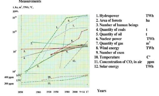
Figure 1: Changings on the World between 1850-2017

Starting Point

According to the United Nations Organization. “As greenhouse gas emissions blanket the Earth, they trap the sun’s heat. This leads to global warming and climate change. The world is now warming faster than at any point in recorded history.” Our opinion is that the situation is not such simple at all. In addition to the Sun’s and the Earth’s own energy, as well as the greenhouse gases, out of which CO2 and methane have already been present since the early life period of the Earth as then probably a reductive condition was, there are different other factors, too, which will be discussed in the subsections. While the incoming energy of the Sun has presumably not changed significantly, in contrast with this the radiated energy of the Earth has decreased. The role of other factors is illustrated by figures and tables in the text and separately in the Appendix, too. Another question is why the greenhouse gas envelope is an obstacle only for the outgoing and not for the incoming energy. In the following part of this manuscript we shell first show the evolution of the life of the Earth.

The Life of the Earth

Before the appearance of biological life, the fate of our Earth was determined not only from its beginning by its own materials and energy but also by those which came from the outside world – the Sun, the cosmos (hereafter: the Sun), too. This process is still going on today, the first stage of which began with the formation of the globe and which was then characterized by an intensive atomic exothermic process. This was the time when atoms were formed. The energy coming then from the Sun, regardless of whether it was the same as it is now or not, had an unknown effect on the Earth’s own energy and processes. This condition could last until the solidification of the Earth’s surface and the appearance of the atmosphere and water. As to the formation of the atmosphere and water we do not know when and how it happened. The water became from H and O and that process had to be exothermic. The radiation of the earth energy decreased due to the subsidence of the internal processes, and intensive energy eruptions could only occur in the form of volcanic activity. In consequence of the changes, the importance of the energy coming from the Sun grew on and on, which until the appearance of biological life could only exert its effect on the Earth’s surface through physico-chemical means in a form corresponding to the greenhouse gases (CO₂ and methane) envelope of that time. This period was the chemical development, during which the conditions for the appearance of the biological life were created.

Life of a living organisms is a biological phenomenon that did not exist before, which arose 3.75/3.8 billion years after the formation of the Earth, in a supposedly reductive environment, and it is nothing other than a continuous and well-regulated energy (electron/ion) migration of different level and complexity, existing in the living beings (from the primordial microorganism and its descendants till the living individuals of today). These primordial bacteria were, for example, chemolithoautotrophs and anaerobes, using CO₂ and other carbon-containing compounds to form methane, or depending on the species, they oxidized sulphur. The electron donor was H. The metabolism of these microorganisms created a new energetic situation, because the energy received from the donor was incorporated into the compounds they produced. With this, the reduction of the amount of atmospheric CO₂ began and the bioenergy and its storage appeared, as well as the transformation of the environment, and its loading with bio-heat and bio-products started. Meanwhile, the Earth continued to radiate its own energy, which, according to geophysicists, currently originates from the Earth’s inner core, and the Sun’s energy continued to arrive in the form of photons (e=h∙f). It is generally believed that, apart from certain fluctuations, the amount of energy reaching the Earth from the Sun can be considered to be the same.

The next stage was the appearance of photosynthesizing microorganisms and the O₂ produced by them, as well as the plants – although trees appeared only 400 million years ago – and the aerobic metabolism. This state resulted in a decisively new situation, because solar energy, which until the photosynthesis only acted on the Earth’s surface through physical-chemical means, since that point of time it has been utilized by the organisms producing their own organic materials, i.e. by storing energy. The essence of this process can be described with the following equation: 6 H₂O + 6 CO₂ + photon = C₆H₁₂O₆ + 6 O₂ and the resulting 1 mol of sugar contains 2,872 KJ of energy. The remains of the dead organisms of that time are the fossil energy sources of today. In the course of continued evolution, higher-order cold-blooded organisms appeared more than 300 million years ago, and then warm-blooded living creatures appeared 230-170 (233?) million years ago. As a result, the load on the environment also increased due to the metabolic products of large animals, which in the case of warm-blooded animals was further increased by the thermal effect, too. The proliferation of herbivorous animals also created favourable conditions for the growth of carnivores. After a biological evolution of 720-770 million years, the first pair of pre-humans appeared in East Africa about 30 million years ago and from there approx. 50,000 years ago, they began to spread throughout the world and the anthropoid period of our Earth began. Humans can be distinguished from animals by their familiarity with fire and its conscious use, (this means the appearance of a new source of increasingly effective energy and CO₂ as well as ash production), the sexual life independent from the estrus and only for pleasure and its aberrations, the domestication and keeping of animals, the accumulation of wealth, the appearance of demands regarding the way of life, the cultivation of plants and the production of consumer goods, the transformation of the environment, the use of means of transport, the utilization of natural energies – water, wind, sun -, the use of nuclear and H energy representing energy sources of increasing importance, and the ability to read/write. As walking on two legs, conscious activity, denaturing nature, use of simple tools, care of offspring, coexistence, communication and some forms of emotional reactions can already be observed in animals, too! The listed energetic and other characteristics that distinguish humans from animals, as well as the high degree of reproduction, the desire for wealth, power and domination, the endless demands and the lack of recognition that we live in a closed system and our possibilities are limited, and the denaturation of nature, as well as the wars which have occurred during the past 224 years have led to the today’s critical state, some of the characteristic energetic and other changes of which are clearly shown in Figure 1. prepared by us in 2015, and as a continuation of it, Figure 3. with the most recent data prepared by the International Energy Agency.

Results

Hydropower

In 2022, 4,289 TWh of electricity was produced by hydropower in the countries of the world, which is 15% of the total amount of electricity and half of the renewable energy (Figure 2). This capacity represents a depreciation compared to the previous period, which was caused by climate change through the drought. The main producers are China (30%), Brazil (10%), Canada (9.2%), the USA (5.8%) and Russia (4.6%). In terms of environmental pollution, this is a clean energy.

FIG 2

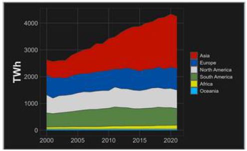
Figure 2: Production of the hydropower-stations between 2000-2020 (Wikipedia)

Forest Area

Based on data from the World Bank, Knoema.com wrote that between 1990 and 2015, 89 countries reported a decrease of their forest area in the last 25 years, 80 countries reported an increase in size of their forests, and 37 countries reported that there was no change. During the mentioned period, the total amount of forests as an extremely important source of energy and raw materials decreased by 1.3 million square kilometres, and the indispensable role of the forests and their bio-systems living there was also lost. The data described here are already included in Figure 1.

Number of People

Since the appearance of man, the number of mankind, even if it has shown significant fluctuations in certain periods, in the end, is constantly increasing. This is confirmed by the following data. 1850: 1.17; 1937: 2.1; 1950: 2.5; 1980: 4.4; 2014: ≈ 7.5 billion. The rate of reproduction shown in Figure 1 is currently accelerating. This can be determined from the following numbers: While on 20 April 2022 the Earth’s inhabitants were 7,944,521,000, on 2 April 2023 there were already 7,993,210,376, i.e. there were 48,686,376 more people. And now, on 27 February 2024, we were 8,093,918,390 because our number increases by one in less than 1 second.

In the beginning, people’s place of residence was less permanent (gathering, fishing, hunting, then grazing period). With the increase in their number and their needs, as well as with the change in their way of life (the spread of farming and domestic animal husbandry), permanent settlements developed and the communal problems related to them appeared. Although cities and even city-states existed in ancient times, urbanization was slow until the period of industrial revolution. The increase in the number of people, the development of agriculture, trade, transport, mining and industry helped the formation of (large) cities. The urbanization process began to accelerate in the 18th century in Europe while on other continents, depending on the circumstances, in the 19th and the 20th century and this process is still taking place today, in many places in an explosion-like form. In 2003, there were 409 cities/agglomerations in the world with more than one million inhabitants. In total, more than 1.15 billion people lived in them, using more than 70% of the world’s resources. Today, more than 50% of our Globe’s inhabitants live in cities, but this proportion varies from country to country. Settlements, especially cities, differ from the natural environment and have a denaturing effect. (With people’s needs, the heat demand, the size and comfort of their homes have also increased compared to those prevalent earlier. The sunlight absorption and heat emission of buildings and roads are different from before. Air pollution, noise and light load have increased. In cities, the so-called “desert climate” prevails). Think about how different the values of individual parameters are over a city with 10 million inhabitants and an area of any natural environment of the same size! It should also be mentioned that currently, the majority of people live in the northern hemisphere of the Earth, which is not surprising for several reasons, but this fact also has its consequences. The rapid increase in the number of mankind is also accompanied by the increasing use of fossil and other energy sources. Without a substantial reduction in the number of mankind and a radical reduction of needs, our situation is hopeless.

Quantity of Coal and Oil Used

As it can be seen on Figure 3 in 2019, after a long increasing the quantity of all fossil energy decreased. In the case of oil, the higher price might also have an influencing effect. The COVID-19 pandemic presumably played a role in the general decline. According to the IEA’s latest report, the amount of oil used was 8.7% more in December 2023 than in December 2022, so growth seems to have started again. They wrote that the demand for coal in 2023 will be greater than earlier with 1,4% and the total quantity will be more than 8,5 billion t-s in the first occasion.

FIG 3

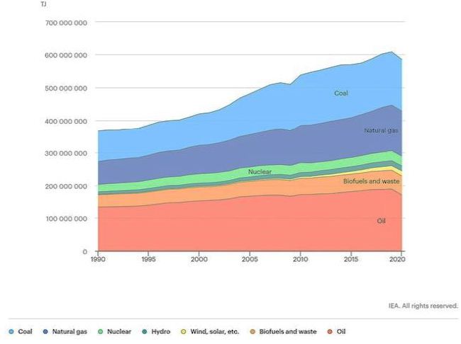
Figure 3: Production and use of different energies on the World between 1990-2020 között (IEA datum)

Nuclear Energy

According to the International Atomic Energy Agency’s annual report published in Vienna, in 2023 there were 438 nuclear power plants operating worldwide with a capacity of 351,327 megawatts, generating 2,447.5 terawatt hours of electricity. In 2019, the amount of electricity produced also decreased. The electricity produced at that time covered 16% of the world’s energy needs. According to the latest IEA report, the amount of electricity produced in December 2023 increased again and was 2.6% more than in December 2022.

The Amount of Extracted Natural Gas

In 2019, the production of natural gas, which had been continuously increasing over the years, also decreased. However, according to the latest IEA report, the amount of gas used in December 2023 was 3.9% more than in December 2022. The reduction in the amount of oil, coal and natural gas used also reduced the amount of CO₂ entering the atmosphere.

Wind Energy

From the beginning of the 2000s, the installation of windpower plants for the utilization of this weather-dependent energy increased dynamically, far exceeding previous expectations, mainly in countries with sea coasts (Table 1).

Table 1: Production of the wind powerstations between 2000 and 2020

Years

Prediction in 2000 Effective production

Difference

2010

85,4 TWh 346,4 TWh*
2020 177,5 TWh 1594 TWh*

Data from 2023 Statistical Review of World Energy

Farm Animals

The number of livestock has increased substantially over the past 100 years, in line with the growth in the number of people and their needs. This is shown by the data in Tables 2 and 3. The increase in the number of animals and changes in husbandry practices have unpleasant consequences (methane, CO2, heat, manure, urine, etc.). According to the latest IEA data, agriculture is responsible.

For about 40% of the methane released into the atmosphere. According to other experts the distribution of sources within agriculture is the following: rice production about 20%, animal husbandry 15-25%, and microbial decomposition of organic matter. According to them, 74% of methane of animal origin comes from cattle, 9% from sheep and 5% from buffalo, and small amounts of the gas are also formed in the rectum of pigs and poultry. These authors do not even mention methane due to the activity of free-living animals and non-animal anaerobic microbes. The IEA estimates that the oil and gas sector contributes about 37% of the methane in the atmosphere, waste contributes about 27% and other sources about 2.8%. They do not mention the release from natural living organisms, or from land and sea due to ice melting (the permafrost phenomenon). If the greenhouse effect of CO2 is 1 unit, that of methane is 21 times greater and that of N-oxides 310 times greater! There is also a view that water vapour has the greatest greenhouse effect. Some of the other consequences of animal husbandry are shown in the Tables in the Appendix. According to IEA experts, methane is responsible for 30% of warming. They also reported that emissions from the oil and gas industry have recently fallen substantially.

Table 2: Number of the different farm animals between 1930-2023

 Time

Animals and their number x 106
  Oxen Horses Pigs Sheep

Hens

1930th

438,9

68,1 193,3 563,0

1999-2000

1351,4 58,2 922,8 1056,1

14860,0

2017

1491,6

60,5 967,3 1202,4 22,8×10³

2021-2023

1913,7 1913,8 1266,0

34.4×10³

Abreviation: – = datum is unknown

Table 3: Number of different farm animals on various continents

Specification

Animals and their number x 106
  Goats Buffalos Donkeys + Mules Camels

’s species*

Europe

17,9

0,2 0,8

Asia

465,2 160,9 18,8 4,2

Africa

218,6

3,4 15,4 15,1

N., C. and S. America

35,8 1,1 7,8**

5,3***

Oceania

0,7

World total in 1999-2000 and in 2017

738,2 165,6 42,8 19,3

5,3

1034,4

200,9 55,3 34,8

Rövidítés: *Lama, alpaca, vicuna és guanaco together; **Datum only from C.-America; ***Datum only from S. -America; -: datum is not known.

Role and Utilization of Solar Energy

The average temperature of the Earth is now largely determined by the amount of energy from the Sun, which is thought to be constant, the amount of which was considered earlier to be 3.86×1033 erg/s, i.e. 3.86×10²³ kW of power. In addition, it is also influenced by the Earth’s own energy and by the effects of the existence of living organisms and the consequences of human activity. Not all of the solar energy emitted reaches the Earth’s surface, because about 30% of the Sun’s energy is reflected from the upper surface of the atmosphere. However, we do not know whether the greenhouse gas envelope has any retention effect and how much, if any. The rest is absorbed by clouds, surface water, ice, snow and land. These represent the Earth’s heat capacity. On the upper surface of the Earth’s atmosphere, in the case of a perpendicular radial position, the energy coming from the Sun represents a power of 1.36 kW/m². The amount of solar energy received and reflected from the Earth’s surface depends on environmental influences. In addition, there is the Earth’s own energy, and the ever-increasing energy generated by the existence and activity of humans or extracted from the Earth by them and emitted by the living organisms. Together, these add up to the total energy under the envelope of greenhouse gases and water vapour. The natural escape of these energies is uniformly retained by the envelope according to the laws of nature, promoting the warming of the Earth’s surface, where ideally the energy input would have resulted in a heat load of 1kW/m², equivalent to 1 kJ/s. This value is the so-called solar constant. We do not know what the solar constant and all the other energy values are today. In 2000, a huge development started in the field of solar energy utilization, because the installation costs of the systems decreased to an unexpected extent and people’s attitudes changed a lot. The annual amount of solar energy collected in the form of electricity between 2012 and 2022 in each year on the world was 104,212; 140,515; 180,712; 228,920; 301,082; 395,947; 489,306; 592,245; 720,429; 861,537 and 1,053,115 MW. It is not known that what is the consequence of the energy captured by the solar collectors on the global temperature?

Occurrence and Role of CO2

As for the CO2 content of the atmosphere, this gas has been present since the early life of the Earth and it is persisting there for a long period of time varying amounts since the beginning (Figure 4). Human life and activity, as well as keeping of livestock and changes in the population of natural living creatures and various geological events, influence the quantity of different gases in the atmosphere. Among these, carbon dioxide, methane, sulphur oxides, water vapour and, more recently, nitrous oxide and fluorine-containing gases have been and are of particular importance because they cause the greenhouse effect and thus accelerate global warming, i.e. climate change. The average concentration of CO2 was in 1750: 250 ppm; in 1957: 315 ppm; in 1987: 350 ppm; in 2015: 403 ppm. On 2 April 2022, atmospheric carbon dioxide concentrations reached their highest level measured at present time at the Mauna Loa monitoring station in Hawaii. The concentration there was 420.86 ppm. Over the Northern Hemisphere 500 ppm was already measured before!

FIG 4

Figure 4: Concentration of CO₂ in the atmosphere (Haszpra László)

The annual amount of CO₂ which was emitted by the countries of the world between 2012 and 2022 in million tonnes per year was 32,219.8; 32,676.8; 32,779.0; 32,773.7; 32,818.0; 33,306.2; 34,013.9; 34,044.0; 32,284.9; 34,052.2; 34,374.1. An average person, if not actively exercising, produces approximately 1kg of carbon dioxide per day that means that worldwide more than 8 billion kg-s, plus the CO₂ which has emitted by animals and then we did not mention the other sources. The year 2020 was the only exception when the steadily rising quantity decreased. The reduction then was the result of the decreasing use of fossil fuels in consequence of the COVID-19 pandemic.

Methane concentrations were in 1700: 1,000 ppb; in 1986: 1,700 ppb; in 2021:
1,875.7 ppb! According to IEA data, the amount of methane released into the atmosphere in 2023 was 349, 476 kt-s and therefore its concentration became more than 1,900 ppb which means a slight increase compared to 2022. This gas persists only for some 10 years in the atmosphere. In spite of the fact that the concentrations of CO₂ and methane which are steadily increasing some people expect and hope the stop of climate change.

The Average Temperature of the Earth

The average temperature of the Earth is influenced by several factors in their own way. These are: the Earth’s own energy, solar radiation, greenhouse gases, the production of previously unknown hydro, wind, solar and nuclear energy, heat from burning fossil raw materials, waste and woody plants, heat emitted by humans, warm-blooded animals and micro-organisms, heat from industry, transport, agriculture, architecture, housing, space exploration, heat from wars and because of the new situation related to denaturing of nature, etc (Figure 6)

FIG 6

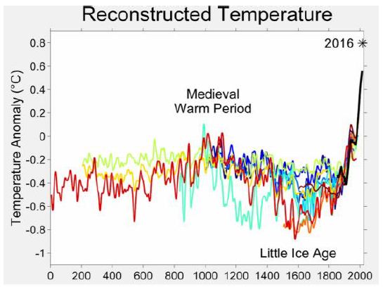
Figure 6: Changing of the temperature of the Earth during last centuries (Wikipedia)

Note: “O” point is equal with some 13,6°C from 1905. Each line was calculated by different expert.
Since the Earth was born, it has been emitting energy, the value of which has decreased over time and is now estimated by experts at between 43 and 49 TW. Without its own energy, the Earth’s temperature would be below freezing point. Despite the supposed ‘uniformity’ of solar radiation, the average temperature of the Earth has never been the same over longer or shorter time periods – see Figure 5. Ice-ages and warming up periods have alternated each other due to terrestrial – chemical, biological, geological and/or, in the present era, human life and activity – or extraterrestrial (?) influences. For example: from the early 1000s there was a so-called little ice age, which was replaced by a warming period due to the changes brought about by the industrial revolution from 1778 on. There is now ample evidence that air and ocean temperatures are rising, snow and glaciers are melting and the sea level is increasing. Between 1905 and 2005, the temperature rose by 0.74 ± 0.18°C every ten years. In the second half of the period under study, the rate of warming doubled compared to the value observed at the beginning (from 0.07 ± 0.02°C to 0.13 ± 0.03°C, per decade). This phenomenon is the so-called climate change. On 21 November 2023, for a short period of time, the Earth’s temperature was already more than 1,3°C warmer (14.9°C) than the global average temperature before the industrial revolution (13,6°C), which was an unprecedented record, reported by the Europe-based Copernicus Climate Change Service. The Earth’s average temperature has been rising for decades as we are facing a self-generating phenomenon because of snow and ice melting, the rising of surface water temperatures, and as the main causes are not diminishing, either, there is little we can do to stop the process [1-11].

FIG 5

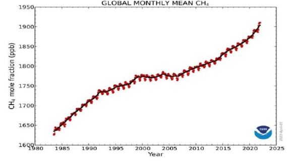
Figure 5: Concentration of methane in the atmosphere (NOAA)

Final Conclusion

We think that a thorough analysis is needed to determine which of the listed factors play a role, and exactly what role, in the climate change process, because in the nature there are no energy changes without effect and causes. So, one of the most important questions is what exactly the role of the greenhouse gas envelope and that of the different factors? In other words, does the current gas envelope affect the amount of solar energy considered to be constant arriving at the Earth’ surface at present compared to its amount which was before the industrial revolution i.e. does the gas envelope have any influence on the incoming energy, or does it just hinder all energies which are present under the envelope in leaving from our environment?. Furthermore, it is a fact that the amount of each of these factors (except the size of forests) are increasing and their energetic and environmental loading importance compared to their 1778 value is steadily growing. Is it conceivable that these changes have no effect? We think the answer is no. Finally, is such view acceptable that the Earth’s own energy within the envelope, together with the solar energy, the biological heat production of the living organisms and the use of non-fossil natural energies by human beings, and the energy release from all combustion processes do not have any effect on the circumstances of our Earth? In our opinion, this is not acceptable, either. If we continue to spend huge amounts of money on goals that are irrelevant to our survival (wars, military investments, unnecessary space exploration, tourism, etc.) instead of stopping climate change and neutralising its consequences, we will miss our chance of survival (Tables 4-6).

Table 4: Data to the circlation of substances and energy on the World

Specification

Years

Mass and average heat value of fuels; Quantity of CO2 liberated from them

1860

1935+37 1958 1980 2000+05 2009+14

2017

Oil × 106t

1

279,5 809,8 3059 3590 4117 4365

40,5 MJ/kg

4,05×10¹⁰ 1,13×10¹³ 3,27×10¹³ 1,23×10¹⁴ 1,45×10¹⁴

1,66×10¹⁴

CO2 m3

3,17×10⁹

8,86×10¹¹ 2,56×10¹² 9,69×10¹² 1,13×10¹³ 1,3×10¹³

Coal × 106t

136 1280 1762 2805 5878 7823

7549

20,35 MJ/kg

2,76×10¹²

2,6×10¹³ 3,58×10¹³ 5,7×10¹³ 1,18×10¹⁴ 1,59×10¹⁴

CO2 m3

3,12×10¹¹ 2,92×10¹² 4,05×10¹² 6,45×10¹² 1,37×10¹³

1,72×1013

Gas × 109m3

71 400 1531 2778 3479 3768

37 MJ/kg

2,62×10¹² 1,48×10¹³ 5,66×10¹³ 1,02×10¹⁴

1,28×10¹⁴

CO2 m3

1,37×10¹¹ 7,72×10¹¹ 2,95×10¹² 5,36×10¹² 6,72×10¹²

All together

MJ/kg

2,8×10¹²

3,99×10¹³ 8,33×10¹³ 1,8×10¹⁴ 3,66×10¹⁴ 4,53×10¹⁴

CO2m3

3,15×10¹¹ 3,94×10¹² 7,38×10¹² 1,9×10¹³ 3,01×10¹³

3,69×10¹³

Abbreviation: – = Datum is unknown

Table 5: Living conditions of different farm animals

Specifications

 Species of animals and their number x million
 Oxen  Horse  Pig  Sheep

 Hen

NEEDS

1 anim. 1351,4 1 anim. 58,2 1 anim. 922,8 1 anim. 1056,1 1 anim. 14860,0

 O2

*calf l/day


390

5,27×10¹¹

*calf l/year

1,42×10⁵ 1,92×10¹⁴

CALORIE
kcal (kJ) x kg0,75 daily  Basal metabolism in case of all animal species in general 70 (293)
yearly  2,55×10⁴ (1,07×10⁵)
kJ x kg0,75 daily  Existential metabolism in case of all animal species 475-575 in general 525
yearly  1,91×10⁵
*calf daily kJ

7712,9

1,04×10¹³

 yearly kJ

2,86×10⁶ 3,8×10¹⁵

 kg**/kJ daily

600/3,5×104

4,77×10¹³ 500/3,09×104 100/9207 50/5400 2/502

 yearly


1,29×10⁷ 1,75×10¹⁴ 1,12×10⁷ 3,36×10⁶ 1,98×10⁶ 1,83×10⁵

 METABOLISM  
kg/W/day

600/411

500/358 100/106 50/62,9 2/5,8

 W/year


1,5×10⁵


1,30×10⁵


3,88×10⁴


2,29×10⁴


2,11×10³


* calf W/day

89,16

* calf W/year

3,25×10⁴

WATER (drinking)  
ml/kg

129

78 108 76

kg/l/nap

600/77,4 500/39 100/10,8 50/3,8 0,25***

kg/l/év

2,82×10⁴

1,42×10⁴ 3,94×10³ 1,38×10³ 73-110

WATER (technological)
l/day


15

l/year

5,47×10³

Abbreviations: *Experimental datum of one calf of 75 kg body weight; **Effective body weight; ***In case of one animal; 1 anim. = one animal; – = datum is not known

Table 6: Emissions of different species of farm animals

Specifications

 Species of animals and their number x million
 

EMISSIONS

 Oxen  Horse  Pig  Sheep

 Hen

1 anim.

1351,4 1 anim. 58,2 1 anim. 922,8 1. anim.. 1056,1 1 anim.

14860,0

CO2 when O2 demand 390 l
*calf l/day

*calf l/year


311

1,13×10⁵

4,2×10¹¹

1.53×10¹⁴


METHANE
l/day

100-500

1,35-6,75×10¹¹  0,3-1,5 2,7-13,8×10⁸ <50


<5,3×10¹⁰


l/year

3,65-18,2×10⁴ 4,94-2466×1011 1,09-5,4×10² 1-5×10¹⁰ <1,8×10⁴


<1,92×10¹³


HEAT when 50%

of metabolism

**kg/ W/day

W/year

600/205,6

7,5×10⁴

2,77×10¹¹

1,01×10¹⁴

500/179

6,53×10⁴

?

?

100/53,2 1,94×10⁴ ?

?

50/31,4

1,14×10⁴

?

?

2/2,9

1.05×10³

?

?

*calf W/day

44,58

6,02×10¹⁰

*calf W/year

1,62×10⁴


2,18×10¹³

WATER
by evaporation g/ 100 kg animal/hour

 240

g/m2/hour

10-200

by perspiration l/hour

some litre

URINE
l/day

10-15

1,35-2,02×10¹⁰ 4-5 2,3-291×108 2,5-4,5  ? 0,6-1,0  ?  –

l/year

3,6-5,4×10³ 7,39×10¹² ? 7,3×10¹¹  ?  ?  ?  ?

 –

FAECES
kg/day

10-30

1,35-4,05×10¹⁰ 15-23 ? 0,5-3 1-3 0,1-0,15 1,48-2,22×10⁹

kg/year

3,6-10,9×10³ 1,47×10¹³ ? ? ? ? ? ? ?

5,4-8,1×10¹¹

Water content in %

80-85

70-80


55-75


55-75

MANURE

kg/animal/day  Is different dependig on the animal species and the way of breeding
SEWAGE
l/day

30***

 4,05×10¹⁰ 1,74×10⁹

l/year

 1,09×10⁴ 1,47×10¹³ 6,3×10¹¹

Abbreviations: *Experimental datum of one calf of 75 kg body weight; **Effective body weight; ***In general 30 l/day in each single animal (500 kg); – = datum is inknown, ? = datum is not written because of the narrow place.

References

  1. United Nations Organization: definition
  2. European Committee (Directorate-general CLIMA): Climate Action.
  3. Food and Agriculture Organization: data
  4. Haszpra László: A bioszféra szerepe a légkör szén-dioxid tartalmának alakulásában. OTKA t042941 zárójelentés, Országos Meteorológiai Szolgálat, Budapest, 2008. in Hungarian
  5. International Energy Agency: data
  6. Központi Statisztikai Hivatal: data in Hungarian
  7. National Oceanic and Atmospheric Administration (USA): data
  8. Ralovich Béla (2020): The History of the Hungarian Nation in the Light of the Life of our Earth. Püski Publishing Co. Budapest, ISBN 978-963-302-292-4
  9. Ralovich Béla (2023) Universe, Space, Infinity, God and our Earth. SciEnvironm 6: 592-610.
  10. Ralovich Béla (2023) Our Thoughts About Social Gender. SciEnvironm 6: 668-672.
  11. Statistical Review of World Energy: data