Abstract
We present a meta-analysis of five Mind Genomics cartographies, done over a 20 year period, all dealing with exercise; purchasing exercise equipment (Buy It!, 2002), joining a branded, well know exercise spa franchised around the US (Curves, 2010), what to say to entice a person to join an exercise club or a gym (2012, student projects at Queens College), and, at the tail-end of a Covid-stricken 2019, how to lure customers back to using exercise equipment either at home and/or the same equipment in a gym (2020). We present the strong performing messages for each cartography, show the power of mind-set segmentation, the power of doing simple background research (student work in 2012), and introduce new foci as well, emotions linked with elements and engagement with messages revealed by response times. These five case histories, the paper shows how Mind Genomics was used by different people in the same ‘general space,’ over a 20-year period, and how Mind Genomics evolved to incorporate new measures alongside its basic measure.
Introduction
We live in a society focused on beauty, whether beauty of the face or of the body, occasionally of the spirit and even of the mind. Whereas among the ancients and their successors in the medieval and modern worlds the search for physical beauty was both artistic and philosophical, today it manifests itself in the world of cosmetics and the world of fitness. One can barely drive through a town, a city, even a rural area without seeing stores devoted to making people more beautiful.
Our focus in this paper is on the world of exercise, a world perhaps not as glamorous as the world of facial beauty and the world of fashion, but a world important, nonetheless. With increasing prosperity and with increasingly caloric intake, coupled with lessened demand on physical activity for work, there is the natural result of increased weight, of lessened body tone. Add that to the oft-feared factor of aging, and one has created a perfect storm for people to focus on what can turn back the clock of time.
The topic of gyms and fitness clubs has enjoyed a moderate amount of published research, and undoubtedly a great deal more one-off business studies deposited after use in the corporate files, presumably hidden away forever, or until the issue has been forgotten along with the research effort. The topics involved in gyms range from a focus on the trajectory of human development [1] to the emotions and motives for joining gyms [2], to health, both physical and psychological [3,4]. At the same time, there is the business aspect of clubs, the need to convince people that certain clubs are worth paying for [5-7].
During the past two decades, as Mind Genomics evolved into the science it is today, a variety of research efforts generated some interesting data on exercise, fitness, and related topics. We look at the salient results from five studies, one run 20 years ago, three run about 10 years ago, and one run a year ago. One study was run to understand how people wanted to shop for exercise equipment. The remaining four studies were run to understand what messages makes people want to join health spas and exercise gyms.
A Short Introduction to Mind Genomics
In 1964, mathematical psychologists R. Duncan Luce and John Tukey had been involved in creating a strong, new, axiom-based foundation for mathematical psychology, and particularly for powerful measurement without using numbers. The approach they developed was called conjoint measurement, the measurement of quantities by the measurement of combinations of such quantities. The approach sounds perfectly ordinary today; measurement mixtures of ideas and from the measurement of the mixtures deduce the measure of the components. The mathematics would appear in a daunting first paper in a new journal, the Journal of Mathematical Psychology, volume 1, number 1, first paper. IN other words, the premier new journal, and the lead article [8].
Conjoint measurement would have remained a stunning intellectual contribution, albeit an esoteric one, except for the efforts of Wharton business school professors Paul Green, Abba Krieger, and Yoram Wind, who would take it, make it practical, and apply it to various problems [9-11]. The literature using conjoint measurement would grow, until the approach would be used for products, for public policy, and so forth [12,13]. One needs only Google(r) the academic literature to get a sense of its applications.
Despite its popularity, most published papers, and indeed most likely research reports buried in corporate offices are one-off studies, executed to solve a particular problem. Conjoint measurement required knowledge of the variables, a painful creation of the combinations, a painful execution, and an analysis, not to mention an equal painful explanation of the method. In other words, the system was expensive, slow, and clunky, reserved for the most important (better read better-funded) project [14].
Mind Genomics emerged out of conjoint measurement, propelled by three key goals:
- Create a system which, like Conjoint Measurement, would be able to measure the strength of ideas by measuring combinations of ideas, so-called vignettes. There was recognition that responses to vignettes could not be easily ‘faked’ as well as the fact that compound messages were more typical in the everyday world than single messages comprising one idea.
- Make sure that each respondent evaluated a unique set of combinations of the same set of elements. This notion of different sets of the same elements emerged from the world of medicine, and the MRI, which takes pictures of the same tissue from different angles, and then recombines them in the analysis phase to come up with a single, 3-dimensional picture [15].
- Create a system which could generate information that would be databased, with the data comparable within a study, and across studies [16].
The studies reported here were run in the same way, following these steps:
- Raw Materials: Create a topic, create a set of questions which ‘tell a story’, and for each question provide a set of ‘answers’ which give different facts. The number of questions can vary but the number of answers for each question is always equal. The Mind Genomics method allows for a variety of such options, such as four questions with nine answers, six questions with six answers, four questions with four answers, etc. The most common study as of this writing (2021) is the design comprising four questions, each with four answers (16 elements).
- Test Combinations: Create a fixed set of combinations, specified as an experimental design The experimental design prescribes the precise set of combinations, doing so by specifying which elements are put together. The experimental design is set up so that the variables are statistically independent, allowing methods such as OLS (ordinary least-squares) regression to reveal how each element or message contributes to the rating assigned to the vignette, viz., to the combination. Respondents do not rate the components; they rate the vignettes, the combinations, which is more natural to them [17].
- Permute the Combination: There are a fixed set of combinations, but the combinations are permuted [15]. For example, one design comprised four questions, nine answers per question, 60 combinations, and many different variations of the underlying design with 60 combinations. This approach lets the ‘experiment’ cover much of the range. Thus, Mind Genomic trades off precision of measuring one small region of the possible combinations of messaging, and instead opts to measure a great deal of the region, albeit with less precision.
- Transform the Ratings in a Way Which Permits Managers to Understand the Results More Easily: In these five studies, four used a 1-9 scale anchored at each end; one used a 5-point scale. Managers who work with the data derived from scale often ask ‘what does a 6 mean’ or a ’4’ mean, etc. To make the data easier for managers to use, consumer researchers and political pollsters have learned transform a scale with many points to a binary scale, no/yes. Following this practice, the researcher transformed the ratings on the 9-point scale to a binary scale (1-6 transformed to 0, ratings of 7-9 transformed to 100). In the case of the 5-point scale, the conversion was 1-3 transformed to 0, 4-5 transformed to 100. In each case, a vanishingly small random number was added to every data point, whether transformed to 0 or to 100, respectively. The random number ensured that no dependent variable would ever be all 0’s or all 100’s for any single individual. This slight variation ensured that the OLS regression always worked for each individual respondent
- Create Equations Relating the Presence/Absence of the Elements to the Newly Created Binary Variables: The experimental design makes it possible to create the equation even with the data of one respondent. Whether the equation is created for a group of respondents, or even for a single individual, the equation is expressed in the same way:
- Uncover Mind-sets: We often divide people by factors that we can easily measure. The easiest of course are WHO a person is, and in today’s digital world, what a person DOES. One can also divide people by the patterns of their answers to sets of questions, the pattern of answers to these questions assigning a person to a group based on attitude. These groups are large, and not particularly actionable. That, knows what a person buys do not tell us what messages move the respondent to buy, and what messages are turnoffs. We don’t typically think like that – viz., having details information about how the world of people’s minds divide for a topic. Usually, the topic is too small, too irrelevant for a deep, detailed investigation.
- Relate the Elements to the Transformed Rating Scale to Show the Impact of Each Element: The OLS (ordinary least-squares) regression analysis uses the data defined by the researcher Once members of the different groups have been identified (viz., respondents belonging to Total, to Males vs Females; to mind-sets 1 vs 2 vs 3), etc. The subgroups are defined either by how the respondent describes himself or herself (done in the context of the study, through self-profiling classification), or the mind-sets are created through clustering and the data from all respondents in a specific mind-set or cluster are combined to create one dataset, and the OLS regression run using all data from that dataset.
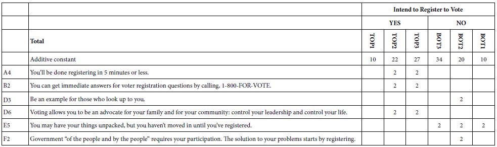
- The additive constant is a measure of the closeness of the vignette to one’s ideal shopping experience, in the absence of elements. The additive constant is purely theoretical, an estimated parameter. It does tell us, however, how positive the respondent is to the shopping experience. The additive constants are all low, between 26 and 34. It will be the elements which will make a difference.
- In most Mind Genomics studies we end up with a few elements which do well. The total panel shows two elements, C2 (Let’s you get your shopping done quickly), and B1 (The price is JUST RIGHT … ALL OF THE TIME). They score 9 and 8, weaker than we will see when we turn to the three mind-sets which emerged from clustering the respondents based upon the similarities among the set of 36 coefficients.
- It will be the mind-sets which show the big differences, differences which suggest three patterns:
- It is mind-sets, not genders, which show the strong responses to the elements, a pattern which shows the power of Mind Genomics to uncover these basic groups in what would seem to be a population which is indifferent to the messages because the first data column. There is no indifference, but rather strong albeit different preference patterns.
- Biedenweg K, Meischke H, Bohl A, Hammerback K, Williams B, et al. (2014) Understanding older adults’ motivators and barriers to participating in organized programs supporting exercise behaviors. The Journal of Primary Prevention 35: 1-11. [crossref]
- Crossley N (2006) In the gym: Motives, meaning and moral careers. Body & Society 12: 23-50.
- Layden T (2004) Get out and play! Like the rest of Americans, school-age children are becoming overweight at an alarming rate. But innovative health experts and gym teachers are introducing kids to the benefits–and joys–of exercise through sports and games. Sports Illustrated 101: 19.
- Otto MW, Church TS, Craft LL, Greer TL, Smits JA, et al. (2007) Exercise for mood and anxiety disorders. Journal of Clinical Psychiatry 68: 669.
- Fogel J, Ustoyev S (2021) Social media advertisements with deposit contracts and fitness club/gym membership: are consumers persuaded? Journal of Consumer Marketing 38: 27-38.
- McKnight OT, Paugh R, McKnight J, Zuccaro L, Tornabene G (2014) Marketing athletic clubs, recreation centers and country clubs: Recruiting and retaining members using psychodemographics. American Journal of Management 14: 60-67.
- Whiteman-Sandland J, Hawkins J, Clayton D (2018) The role of social capital and community belongingness for exercise adherence: An exploratory study of the Cross Fit gym model. Journal of health Psychology 23: 1545-1556.
- Gustafsson A, Herrmann A, Huber F (2000) Conjoint analysis as an instrument of market research practice. In Conjoint measurement 5-45. Springer, Berlin, Heidelberg.
- Green PE, Wind Y, Carmone FJ (1972) Subjective evaluation models and conjoint measurement. Behavioral Science 17: 288-299.
- Green PE, Krieger AM, Wind Y (2001) Thirty years of conjoint analysis: Reflections and prospects. Interfaces 313: S56-S73.
- Krieger AM, Green PE, Wind Y (2004) Adventures in conjoint analysis: A practitioner’s guide to trade-off modeling and applications. Monograph, University of Pennsylvania.
- Milutinovic V, Salom J (2016) Mind Genomics: A Guide to Data-Driven Marketing Strategy. Springer.
- Moskowitz HR, Gofman A (2007) Selling Blue Elephants: How to Make Great Products That People Want Before They Know They Want Them, Pearson Education.
- Wind J, Green PE, Shifflet D, Scarbrough M (1989) Courtyard by Marriott: Designing a hotel facility with consumer-based marketing models. Interfaces 19: 25-47.
- Gofman A, Moskowitz H (2010) Isomorphic permuted experimental designs and their application in conjoint analysis. Journal of Sensory Studies 25: 127-145.
- Moskowitz HR, Gofman A, Beckley J, Ashman H (2006) Founding a new science: Mind genomics. Journal of Sensory Studies 21: 266-307.
- Moskowitz HR (2012) ‘Mind Genomics’: The experimental, inductive science of the ordinary, and its application to aspects of food and feeding. Physiology & Behavior 107: 606-613.
- Likas A, Vlassis N, Verbeek JJ (2003) The global k-means clustering algorithm. Pattern recognition 36: 451-461.
- Schwartz B (2004) January. The paradox of choice: Why more is less. New York: Ecco.
- Bergert FB, Nosofsky RM (2007) A response-time approach to comparing generalized rational and take-the-best models of decision making. Journal of Experimental Psychology: Learning, Memory, and Cognition 331: 107.
- Rubinstein A (2013) Response time & decision making: An experimental study. Judgment and Decision Making 8: 540-551.
For those experiment designs using the 4×9 structure (four questions, nine answers for each question): Binary Variable (TOP3) = k0 + k1(A1) + k2(A2) … k36(D9)
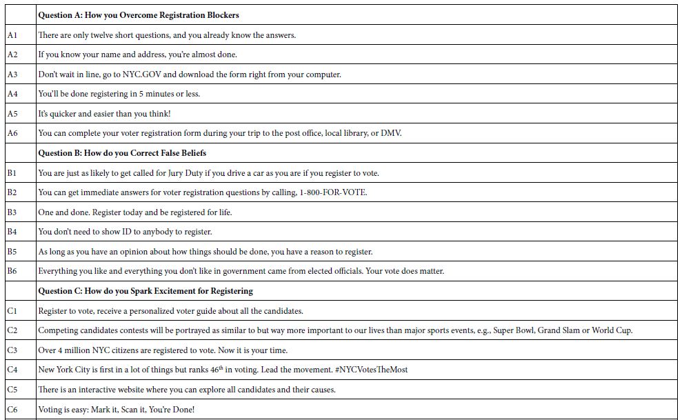
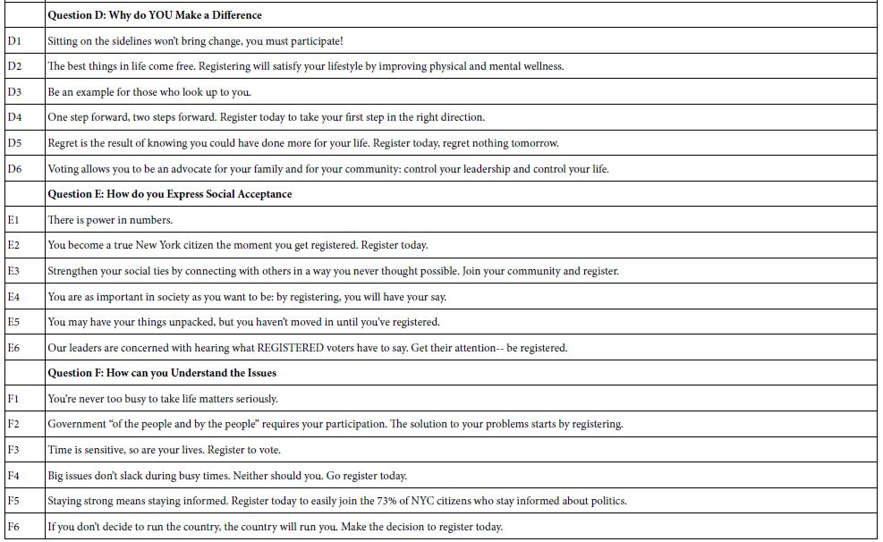
For those experimental; designs using the 6×6 structure (six questions, six answers for each question):
Binary Variable (TOP3) = k0 + k1(A1) + k2(A2)… k36 (F6)
For those experimental design using the 4×4 structure (four questions, four answers for each question): Binary Variable (Top2) = k0 + k1(A1) + k2(A2) … k16(D4)
Mind Genomics create different groups of people, not based on who they are, but rather on the pattern of their reactions to limited types of information. That is, the division of people is not based on the way the person thinks about large (and important) problems, buts divides people on the pattern of responses to any topic, in ways which make sense. The method is called clustering [18]. Clustering is based upon mathematical criterion. However, the choice of the number of clusters to use is based upon two non-mathematical criteria. The first is parsimony – fewer clusters are better than more clusters. The second is interpretability – the clusters must tell a coherent story. Parsimony and interpretability are opposed; more clusters mean easier to tell a story, but only the truly relevant elements need be included in the cluster.
Cartography 1 – Buying Exercise Equipment
Study # 1 was done in 2002, just about 20 years ago. The study was part of a large group of studies which focused on the nature of messaging which represent one’s idea shopping experience [13]. Figure 1 shows the wall of studies. All studies were identical except for the name of the product, and certain features and stores. The respondent selected the study and was led to the introduction for that study shown in Figure 2.

Figure 1: The wall of studies for Buy It! the respondent selected the study.

Figure 2: Respondent instructions for the Buy It! Study. The introduction comes from the study dealing with exercise equipment.
The different studies in the Buy It! project comprised four questions or silos, each with nine answers or elements. We will use the term element instead of answer. The 4×9 design (four questions, nine answers) generate 36 elements in total, combind according to an underlying experimental design into 60 vignettes. Each element appear an equal numbr of times across the 60 vignettes. Furthermore, the vignettes comprised 2-4 elements, so by design many of the vignettes were ‘incomplete,’ viz.,lacking an answer from one of the four questions. As noted above, each respondent evaluated a unique set of combinations, permutations of the original design.
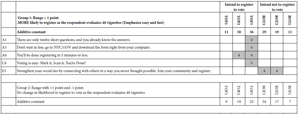
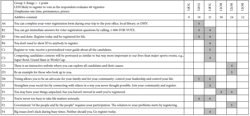
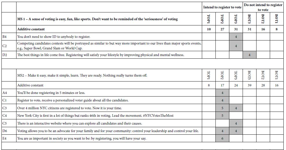
Table 1 shows only those elements which exhibit at least one strong performing element. The element had to have an estimated coefficient of +8 or higher when the dependent variable was defined as a binary scale (1-6 → 0; 7=9 → 100). Table 1 thus shows the highlights. We show the elements first in terms of total panel, then in terms of three mind-sets to emerge, and then in terms of gender.
Table 1: Strong performing element for the 2002 Buy It! study on exercise equipment. (Table courtesy of It! Ventures).
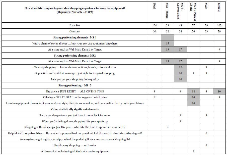
a. Mind-Set 1 responds to the stores
b. Mind-Set 2 convenience
c. Mind-Set 3 wants price and choice.
Cartography 2 – What Messages Drive Women to Say that They Will Join Curves
Study # 2 was run in December 6-7, 2010, at the behest of Queens College, in collaboration with author HRM, and the mathematics department of Queens College. The study was part of the ‘vetting processes that Queens College used to create a mathematics course, Math 110, offered 2011-2013. Two of the owners of a local gymnasium were interested in signing up with Curves. They approached Queens College and funded the study, which was otherwise done on a pro bono basis with permission to publish the results of the study in two years.
The ingoing brief for the study was the following:
To prosper in the present economy Curves Owners must always be on the look-out for new ways to accommodate and engage their members. Curves owners need faster access to useful consumer insights in developing marketing messaging and programs, products and services. The Vision – Increase lasting memberships at Curves. The marketing and sales strategy to emerge from Mind Genomics was set forth at the set-up meeting:
Attract prospects to come into your club by using optimum message appearing to the general marketplace through: Web coupons, Mailing Value Coupon packs, Web site landing page, E-mails, In person
When the prospect comes in, lead the discussion with those Curves features that appeal most to each individual: Use a simple approach to tell you EXACTLY what to say to each individual
Study # 2 was run on December 6-7, 2010, with a population of women of all ages across the US. The raw material for the study came from current (2010 basis) marketing and advertising messaging from Curves website as well as from websites of peer fitness clubs: Butterflylife, Contours express, Fitness club Forwomen, and Lady of America, respectively.
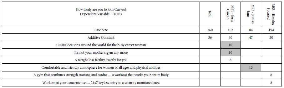
Table 2 shows the strong performing elements for the study. There were 36 elements. Surprisingly, most of the elements fared quite poorly. That is, despite their use in the promotional literature, their actual performance was poor using the criterion of consumer reactions. This is often the finding of a Mind Genomics study, perhaps because the elements used have not been established ‘effective’, in a rigorous, unbiased manner. That is, most elements used in the study may well have been legacy elements, the origin and usefulness of lists lost if, in fact, they are really existed.
Table 2: Strong performing elements for the ‘Curves’ study.
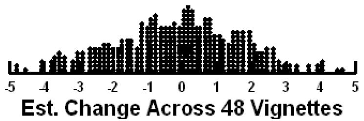
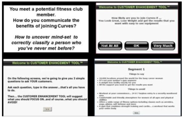
A key benefit of the Mind Genomics approach is the ability to assign new people to the appropriate mind-set. This is done with the PVI (Personal Viewpoint Identifier). The PVI uses statistical methods such as DFA (Discriminant Function Analysis), and Decision Trees to create a limited set of questions emerging from the elements or answers of the study. These are the elements which best differentiate the mind-sets from each other. Figure 3 shows an example of how the PVI appears in 2010, summarizing the process. The figure shows the objective, the respondent introduction (left column), and then one of the three questions and one of the three outputs (right column). The new respondent completes a short set of questions. The pattern of responses to the questions suffices to assign that respondent to one of the three mind-sets just uncovered. The process lasts about 30-45 seconds.
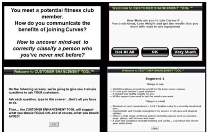
Figure 3: The PVI (Personal Viewpoint Identifier), showing the introduction. one question (of three) from the PVI, and the feedback when the respondent is assigned to Mind-Set (Segment) 1. The figure shows the version of the PVI from 2010.
Cartography 3 – Joining a Fitness Club
Study #3 (as well as Study #4 on joining a gym) was done in 2012 at Queens College by a cadre of four students in the Math 110 course. The course was an experiment run for five semesters at Queens College of City University of New York. The idea was to teach the students a combination of critical/creative thinking with a dose of mathematics and mathematical thinking. The students were divided into groups of four individuals, instructed on the basics of Mind Genomics (at that time called Addressable Minds for business), and selected a topic. The two studies reported here, chosen by two separate groups of students, show the power of creative thinking, and the strong performance of the elements when the students were engaged in research, and challenged to do their best.
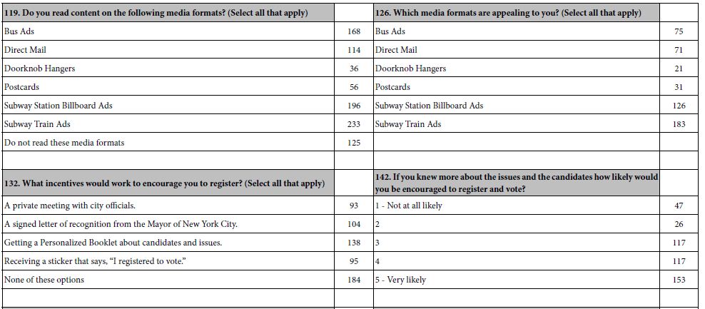
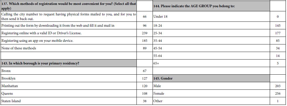
Figure 4 shows the orientation page to the study and is similar to the orientation pages of previous studies. The student was interested both in what drives interest in joining a fit club (question #1), as well as the emotional reaction to after reaching each vignette (question #2). This presentation of data from Study # 4 focuses only on the data from Question #1 (joining) to demonstrate the richness of the results. Emotions will be shown in the next study on joining a gym (Cartography #4).
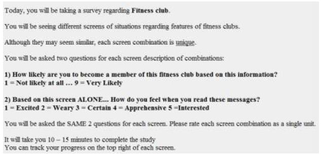
Figure 4: The orientation page to the study on joining a fitness club.
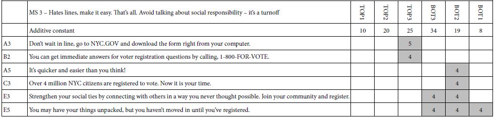
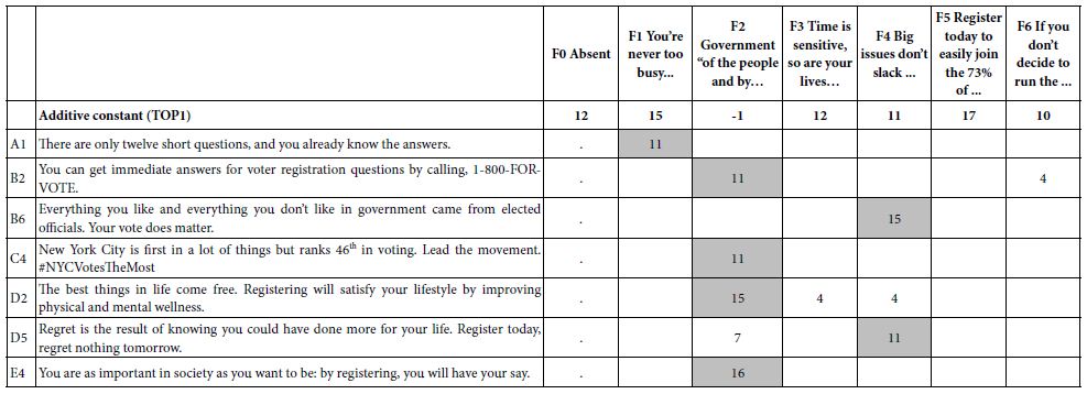
The actual design was a so-called 4×6 (four questions, six answers). Table 3 shows the strong performing elements by total panel, by gender, and by four emergent mind-sets. One mind-set, MS1, is very small, and should be discarded, but we leave it here for completeness. What emerges as remarkable in light of the previous two studies in the richness of the results, something that will be seen in the next study as well on joining a gym? The reason for the richness can be principally attributes to good up-front thinking by the four students who participated. The students took the project seriously, looked at the different messaging on the Internet, selected what seemed to be reasonable, and put that messaging into the study. The results, with 50 respondents, are no less than spectacular, with the number of very strong performing elements.
Table 3: Performance of elements for joining a fitness club.
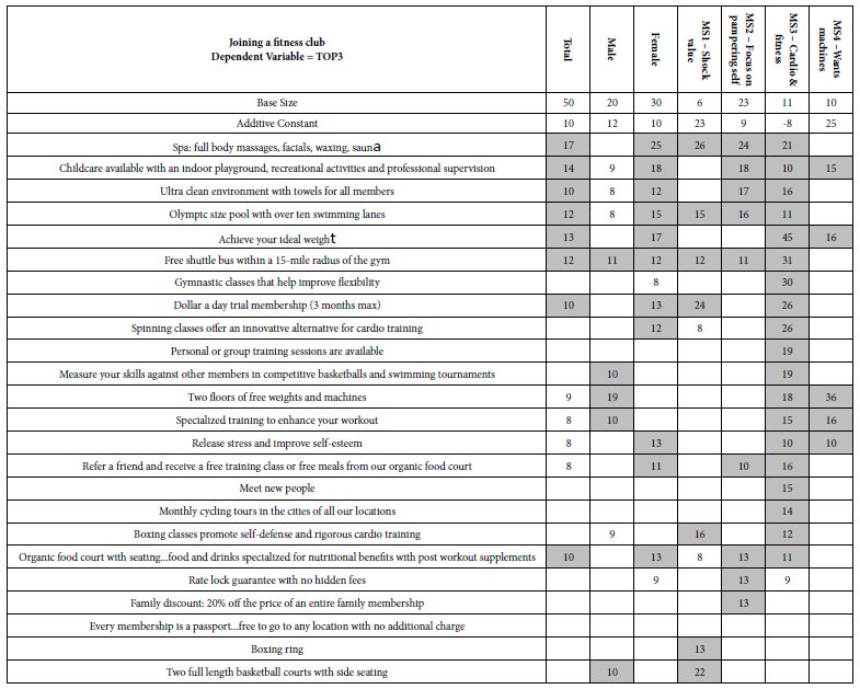
Mind-Set 1: Very modestly interested (additive constant 29), but attracted by the ‘shock’ value of services and prices
Spa: full body massages, facials, waxing, sauna
Dollar a day trial membership (3 months max))
Mind-Set 2: Barely interested (additive constant 9) but attracted by some outstanding features
Spa: full body massages, facials, waxing, sauna
Child-care available with an indoor playground, recreational activities and professional supervision
Ultra clean environment with towels for all members
Olympic size pool with over ten swimming lanes.
Mind-Set 3: Basically disinterested (additive constant -8) but exceptionally interested in cardio and fitness, as well as making it part of an easy daily schedule
Achieve your ideal weight
Free shuttle bus within a 15-mile radius of the gym
Gymnastic classes that help improve flexibility
Dollar a day trial membership (3 months max)
Spinning classes offer an innovative alternative for cardio training.
Mind-Set 4: Modestly interested (additive constant 25), and want machines for self-training
Two floors of free weights and machines.
The words of the four students are especially relevant here to summarize the results, and to show how new-to-the-approach students can learn to think more deeply about the topic.
“Addressable Minds was able to help identify the immense importance the therapeutic effect can provide to its members in a fitness center. Mostly overlooked, due to cardio and weightlifting but equally important to fitness and health is the state of the mind and spirit. The high response rate for the “Spa” and “Organic Food Court” elements demonstrate members are seeking more than just a weight room. Eating the right food along with properly relaxing the mind and body allow members to perform better in the gym thus maximizing the results. Providing these added qualities are crucial to health inside and out but also allow members to get more out of it than a traditional fitness center. Furthermore “Child Care” allows the member to escape responsibilities for a time, to truly focus on strengthening the spirit and mind.”
Cartography #4: Joining a Gym
Study # 4 was done at the same time as Study # joining a health club, but by a different team of students in the same class, Math 110 in Queens College. The process was the same and the instructions were virtually the same except that the work ‘gym’ replaced the phrase ‘fitness club’.
The data for this fourth cartography once again shows the power of doing one’s homework, of taking messages from competition. Table 4 shows low additive constant (-6) suggesting that it is the specifics of the gym which make a difference, not the basic interest in the gym. Table 4 also shows that the additive constant is higher for males (+24) and vanishing low for females (-16). For females, it will be the elements which must do the hard work to convince.
Table 4: Performance of elements for joining a gym.
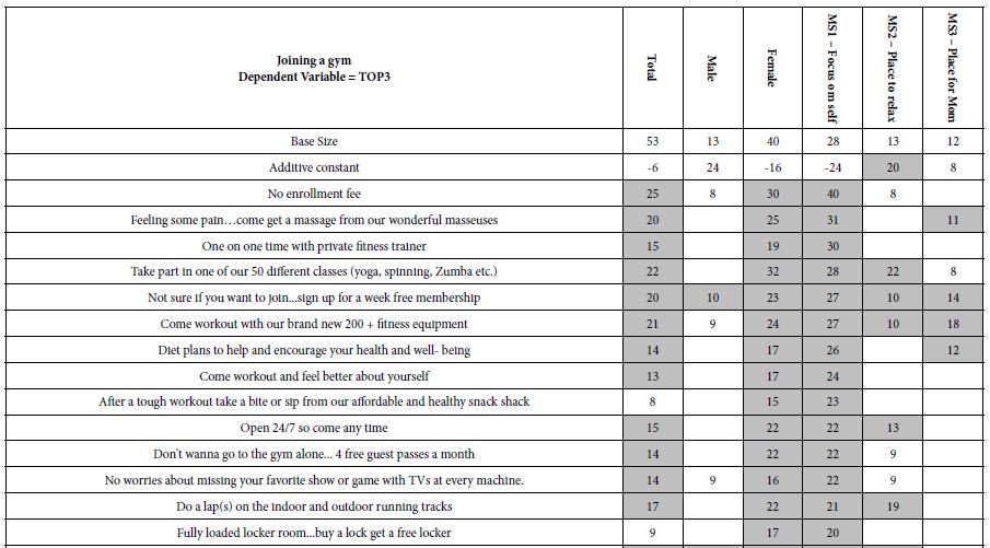
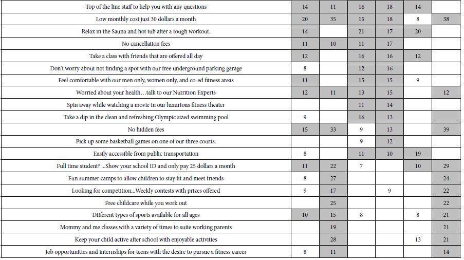
The data becomes, more interesting when we look at the three mind-sets which emerge.
Mind-Set 1 is basically uninterested in the gym but strongly differentiates among the messages, and actually loves most of the messages except for those dealing with children. The elements interesting Mind-Set 1 are:
No enrollment fee
Feeling some pain…come get a massage from our wonderful masseuses
One on one time with private fitness trainer
Take part in one of our 50 different classes (yoga, spinning, Zumba etc.)
Not sure if you want to join…sign up for a week free membership
Come workout with our brand new 200 + fitness equipment
Diet plans to help and encourage your health and well- being.
Mind-Set 2 likes the notion of joining a gym, although again it is what the gym offers (additive constant 20). The key elements interesting Mind-Set 2 are:
Take part in one of our 50 different classes (yoga, spinning, Zumba etc.)
Relax in the Sauna and hot tub after a tough workout.
Mind-Set 3 has no predisposition to joining the gym (additive constant 8) but like a low price. Their response show that they are the opposite of Mind-Set 1, viz., interested in an activity with their children. The elements interesting Mind-Set 3 are:
Low monthly cost just 30 dollars a month
Full time student? …Show your school ID and only pay 25 dollars a month
Fun summer camps to allow children to stay fit and meet friends
Looking for competition…Weekly contests with prizes offered
Free childcare while you work out
Different types of sports available for all ages
Mommy and me classes with a variety of times to suit working parents
Keep your child active after school with enjoyable activities.
Table 5 shows how the elements link with the choice of emotion. The analysis of the emotion responses was slightly different from the analysis of the ratings for joining. Recall that for the reactions about joining, the 9-point rating scale was converted to one binary variable, taking on the value ‘0 when the original rating was 1-6, and taking on the value ‘100’ when the original rating was 7-9.
Table 5: Strong linkages (>=8) between elements and selected emotion for the cartography on selecting a gym.
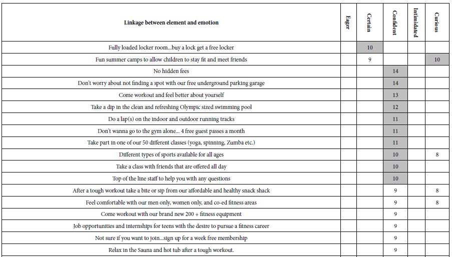
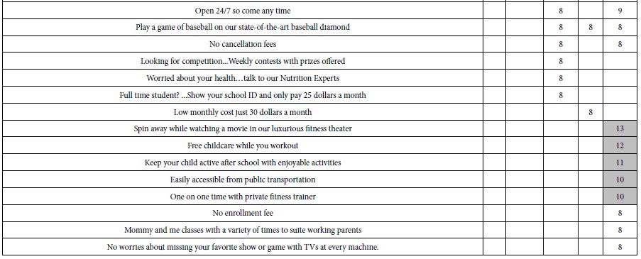
This type of transformation does not work for the emotion scale, known as a ‘nominal scale.’ The numbers are simply placeholders for different, not necessarily related emotions. The solution, simple and in the same spirit, was to create FIVE new binary variables, one binary variable for each of the five emotions. A selection of an emotion for a vignette would result in the value ‘100’ for the newly created binary variable corresponding to that emotion, and the value ‘0’ for the four new created binary variables corresponding to the emotions not selected. For example, when the respondent selected the emotion ‘5’ (Interested), the newly created binary variable ‘INTERESTED’ was assigned a value of ‘100’ and the remaining four binary variables (EXCITED, WEARY, CERTAIN, APPREHENSIVE) were all assigned a value of ‘0’. The vanishingly small random number (<10-5) was added to each newly assigned value, whether ‘0’ or ‘100’, respectively.
The regression analysis relating the presence/absence of the elements to the selection of the emotion was run separately five times, once for each of the five newly created vignettes. The equation was the now familiar regression equation, but the equation was absent the additive constant. The rationale is that the additive constant would be the same for the five newly created binary variables and provides no additional information.
The two emotions selected most often are confident and curious. Only the strong linkages are show, 8 or higher. The emotion confident links with elements giving the respondent control and choice:
No hidden fees
Don’t worry about not finding a spot with our free underground parking garage
Come workout and feel better about yourself
Take a dip in the clean and refreshing Olympic sized swimming pool
Do a lap(s) on the indoor and outdoor running tracks
Don’t wanna go to the gym alone… 4 free guest passes a month
Take part in one of our 50 different classes (yoga, spinning, Zumba etc.)
Different types of sports available for all ages
Take a class with friends that are offered all day
Top of the line staff to help you with any questions.
The emotion curious links with diversion (movie), children, easy to access, and a personal trainer
Spin away while watching a movie in our luxurious fitness theater
Free childcare while you workout
Keep your child active after school with enjoyable activities
Easily accessible from public transportation
One on one time with private fitness trainer.
The new learning here is that by linking emotion with the elements, one begins to get a deeper sense of why the elements seem to do well. The respondent may not be able to articulate the reason for choice, but the nature of the linked emotion may provide that insight.
Cartography 5: Gym-Two-Ways (2020)
Study #5 was done in late 2020, during the waning period, after the height of the lockdown due to Covid-19. The objective was to see what type of basic messages would attract prospective customers, who had just been through the lockdown, and might be interested in return to a gymnasium, or having a home trainer work with them using the same equipment in their home.
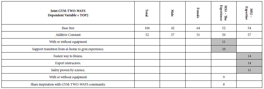
By 2020 Mind Genomics had transitioned to the much easier to use 4×4 design, comprising 16 elements (four answers each to four questions) The design generated 24 vignettes, which were permuted by the standard permutation approach, so that across the 106 respondents many of the possible vignettes were estimated. The rating scale was also reduced from 9 points to 5 points. The total time for the Mind Genomics exercise went from about 15 minutes to 3 minutes
Table 6 shows a much-reduced set of strong performing elements. There are still themes emerging, but what is important is the reduced set of strong performers, and the much lower coefficients. The reason for this may be the emergence of a society whose ability to concentrate on messages and to become excited has diminished and continues to diminish. It may well be that over the period of a decade the prospective audience has been saturated, the so-called paradox of choice [19]. That paradox may reveal itself in what might be called a customer-based ennui, and a growing indifferent to messaging.
Table 6: Performance of elements for GYM-TWO-WAYS.
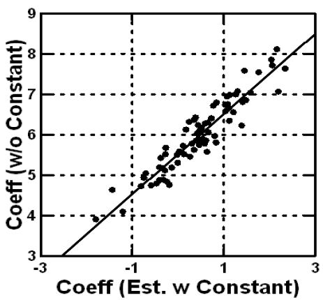
Our final analysis concerns response time. The Mind Genomics program recorded the interval between the presentation of the vignette and the respondent’s rating. The interval is called the response-time, and presumably co-varies with internal psychological processes, including reading and decision-making [20,21]. We can look at the estimated response time of each element, with the estimation coming from the OLS (ordinary least-squares regression). Once again there is NO additive constant.
Table 7 shows the longest and the shortest response times. Most response times are between 0.5 and up to, but not including one second. Only a few elements are processed very quickly or processed more slowly than the half-second range between 0.5 and 1.0 seconds.
Table 7: Estimated response time for elements. Only the ‘short’ and the ‘long’ response times are shown.
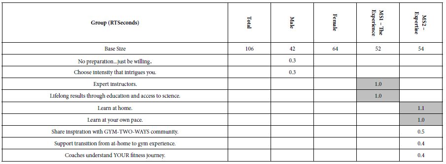
Elements that are quickly (estimated response time <= 0.4 seconds)
No preparation…just be willing (males)
Choose intensity that intrigues you (male)
Share inspiration with GYM-TWO-WAYS community. (MS2 – Expertise)
Support transition from at-home to gym experience. (MS2 – Expertise)
Coaches understand YOUR fitness journey. (MS2 – Expertise)
Elements processed slowly (estimated response time >= 1.0 seconds).
Expert instructors.(MS1 – Experience)
Lifelong results through education and access to science. (MS1 – Experience)
Learn at home. (MS2 – Expertise)
Learn at your own pace. ( MS2 – Expertise).
Discussion and Conclusion
During the past six decades, since the early and middle 1960’s, researchers have focused on obtain increasing amounts of information from customers. Sixty years ago, it was sufficient to measure general attitudes towards products, desires for certain features, and perhaps the ‘gap’ between what was being offered and what was desired by consumers. This so-called ‘gap-analysis’ was satisfactory but over time the world of consumer goods and services would evolve to cut-throat competition. New methods were needed to understand the competitive frame.
The heyday of consumer research saw the development of new ways to understand the mind of the consumer. In terms of goods and services, Professors Paul Green and Yoram Wind at Wharton pioneered the methods of experimental design to study the trade-offs that consumers would make when considering a service or a product. The notion of trade-off was not new, but the zeitgeist of the 1970’s was moving towards the study of mixtures as being the natural stimuli.
It is in the spirit of this movement towards studying mixtures that Mind Genomics was born. The objectives were no longer to do single, difficult-to-execute studies, but rather to create a system that would be able to produce knowledge on demand for verticals such as buying products (Buy It!, source of the study on exercise equipment), or solutions to practical problems at the time, at low cost, with cycle times per iteration of a day or less (Curves, GYM-TWO-WAYS), or teaching tools, forcing first-year, non-quantitatively oriented college students to research the competitive frame, and to run a study which both taught them how to structure their inquiry, and how mathematics could provide important information.
The studies here represent a collection of different issues, done by different researchers, at different times. The numbers are comparable. The coefficient is the percent of respondents saying ‘yes’. Thus, there is ongoing learning, revealed by the meta-analysis, the learning transcending the specific elements, and in addition showing how nature of the up-front research may provide information of higher value.
References