DOI: 10.31038/EDMJ.2025941

Abstract

A 51-year-old man with hypertension and diabetes presented with proximal muscle weakness and severe hypokalemia. Hormonal evaluation confirmed ACTH-dependent Cushing’s syndrome, with extremely elevated cortisol levels (>1100 ng/ml), consistent with a severe form of the condition. Imaging and biopsy identified an ectopic ACTH-secreting thymic neuroendocrine tumor (atypical carcinoid) with chromogranin A positivity. Initial medical therapy with fluconazole failed to reduce cortisol levels. To mitigate perioperative risk from hypercortisolemia, a low-dose overnight etomidate infusion was initiated, successfully lowering cortisol levels below 300 ng/dl. Surgical excision of the tumor was then performed. Histology confirmed atypical carcinoid with a Ki-67 index of 7.5%, and evidence of capsular and vascular invasion. Postoperatively, cortisol and ACTH levels dropped significantly, and the patient was started on physiological hydrocortisone replacement. He experienced no complications from cortisol excess and is currently being monitored for disease re-staging. The case underscores etomidate’s value in preoperative cortisol control in severe ectopic Cushing’s syndrome.

Keywords

Ectopic Cushing’s syndrome, Atypical thymic carcinoid, Etomidate, Severe Cushing’s syndrome

Background

Ectopic Cushing’s syndrome is a rare condition that contributes to 10-20% of Adrenocorticotropic Hormone (ACTH)-dependent Cushing’s syndrome cases. Severe Cushing’s syndrome, which is defined when serum cortisol levels are above 1100 ng/ml, is rare in ectopic Cushing’s syndrome and carries higher perioperative and postoperative morbidity and mortality. Distinguishing ectopic Cushing’s syndrome from other causes of Cushing’s syndrome is imperative, as removing the tumor can cure the condition. Normalizing cortisol levels prior to surgical removal is crucial to reduce peri- and postoperative morbidity and mortality.

We present a case of severe ACTH-dependent Cushing’s syndrome due to an ectopic ACTH-secreting atypical thymic carcinoid tumor, which we successfully treated with etomidate pre-operatively, leading to good postoperative outcomes. In environments where intensive care facilities are scarce, high-dependency units (HDUs) may offer a safe and effective alternative for administering low-dose etomidate infusion to manage hypercortisolemia. In this particular case, serum cortisol levels were successfully reduced to approximately 300 nmol/L without inducing cardio-respiratory compromise.

Pre-operative etomidate prior to definitive surgical treatment of thymic carcinoid tumors helps to minimize complications.

Introduction

Hypercortisolism and the range of symptoms associated with it are collectively referred to as Cushing’s syndrome. Exogenous Cushing’s syndrome is the most common type, while endogenous Cushing’s syndrome occurs secondary to excess cortisol, which may be due to ACTH-dependent and ACTH-independent mechanisms. ACTH-dependent causes account for 70–80% of cases, while 20–30% of cases are ACTH-independent. ACTH-dependent Cushing’s syndrome can occur due to pituitary tumors or tumors at ectopic sites, and ACTH-independent Cushing’s syndrome is usually caused by adrenal lesions [1,2].

Ectopic Cushing’s syndrome is a rare condition contributing 5-20% of all Cushing’s syndrome cases and 10-20% of all ACTH-dependent Cushing’s syndrome cases. The commonest sites for ectopic ACTH secretion are the lung, mediastinum, gastro-entero-pancreatic neuroendocrine tumors, or pheochromocytomas, respectively [3].

Severe Cushing’s syndrome is defined by random serum cortisol levels more than 40 μg/dL (1100 nmol/L) at any time or a 24-hour urinary free cortisol more than fourfold the upper limit of normal and/or severe hypokalemia (<3.0 mmol/L). Severe hypercortisolism is associated with a higher risk of infection, septicemia, thromboembolism, and postoperative morbidity compared to mild and moderate Cushing’s syndrome. Thus, reducing hypercortisolism at the time of intervention may benefit these patients. Depending on the lesion site, we can categorize the available treatment options into medical, surgical, and radiotherapy-related treatments. It’s pivotal to differentiate ectopic Cushing’s syndrome from other causes because identification of the ectopic site and surgical removal may completely cure the disease [4].

We present a case report on a 51-year-old Sri Lankan male who was diagnosed with severe ACTH-dependent Cushing’s syndrome secondary to ectopic ACTH-secreting atypical thymic carcinoid tumor. He was successfully treated using low-dose etomidate with minimal postoperative complications. This case report highlights the benefits of preoperative low-dose etomidate treatment, leading to a successful postoperative outcome in managing severe hypercortisolism. Also, in environments where intensive care facilities are scarce, high-dependency units (HDUs) may offer a safe and effective alternative for administering low-dose etomidate infusion to manage hypercortisolemia. In this particular case, serum cortisol levels were successfully reduced to approximately 300 nmol/L without inducing cardio-respiratory compromise.

Case Presentation

A 51-year-old male who is a known patient with well-controlled diabetes mellitus and hypertension presented with the complaint of episodic diarrhea over a 2-week duration and difficulty in standing from a squatting position, suggesting proximal muscle weakness. He also had sinister lower back pain that was persistent throughout the day with the same intensity, with no recent history of trauma. He noted facial flushing and mild facial puffiness along with exertional shortness of breath and excessive tiredness with routine tasks.

He had severe constitutional symptoms, including weight loss of nearly 10 kg over the last 2 months with loss of appetite. The patient denied any recent onset of pigmentation, palpitations, episodic flushing, or wheezing episodes in the recent past. The patient complained of visual and auditory hallucinations with depressive symptoms, episodically over the last two months. There were no visual disturbances, history of dyspeptic symptoms, renal stone disease, or any family history of similar disease to suggest multiple endocrine neoplasia (MEN) syndrome.

On examination, the patient had a BMI of 19.53 kg/m² with an initial blood pressure of 180/100 mmHg. He had flushing involving the face and upper chest with thin skin and subtle nail hyperpigmentation. Overt clinical signs of Cushing’s syndrome, including buffalo hump, purple abdominal striae, or hirsutism, were not seen. The patient exhibited proximal muscle weakness with a power of 3/5 in both the upper and lower limbs, in contrast to distal muscle power, which was 4/5. His mental status examination revealed visual and auditory hallucinations with a moderate degree of depression. Throughout the hospital stay, it was noted that he had poor blood pressure control with evidence of resistant hypertension and poor glycemic control (Table 1).

Table 1: Investigations

White cell count	14.98 × 109
Hemoglobin	11.7 g/dL
Platelet count	238 × 103
Serum sodium	141 mmol/L (136-145)
Serum potassium	2.1 mmol/L (3.5-5.1)
Erythrocyte sedimentation rate	45 mm/1st hour
Aspartate transferase	58 U/L (11-34)
Alanine transaminase	145 U/L (<45)
Total Bilirubin	1.9 mg/dl
Direct Bilirubin	1.0 mg/dl
Alkaline phosphatase	350 mu/L
Gamma-glutamyl transferase	284 mu/L
Albumin	2.1 g/dL
Globulin	2.7 g/dL
9am cortisol (initial)	1220 nmol/l (118.6-618)
9am cortisol (Post fluconazole for 1 week)	1100 nmol/L
Overnight dexamethasone suppression test (ODST)	880.33 nmol/L (≤50)
Low dose dexamethasone suppression test (LDDST)	260.3 nmol/L (≤50)
Cortisol day curve	9am 674.95 nmol/L
	11am 1038.61 nmol/L
	3pm 760.38 nmol/L
	5pm 797.55 nmol/L
Adrenocorticotrophic Hormone (ACTH) level	172 pg/ml (4.7-48.8)—— 81 pg/ml (Post operatively)
Albumin corrected Calcium	8.9 mg/dL (8.6 to 10.3 mg/dL)
Serum Prolactin	203.24 mIU/L (73-412)
Abdominal ultrasound (USS)	Normal USS abdomen with no evidence of organomegaly or adrenal lesions.
Contrast-Enhanced Computed Tomography (CECT) chest- abdomen- pelvis	Lobulated soft tissue density lesion in the anterior mediastinum measuring 3.3 cm × 4.8 cm × 5 cm. Lesion shows avid contrast enhancement with internal non-enhancing areas. No calcifications. It compresses the left subclavian vein posteriorly, and in-between fat planes are obliterated. Fat planes between the lesion and SVC are also obliterated. Enlarged lymph nodes are seen in the right lower paratracheal and upper paratracheal regions.
USS guided FNAC of the mediastinal lesion	Cellular smears reveal epithelial clusters and single cells with acinar arrangement and sheets. Nuclei are prominent with fine speckled chromatin with a few enlarged nuclei and eosinophilic cytoplasm. No admixed lymphocytes or keratin pearls. Ki67 30% Suggestive of neuroendocrine carcinoma of the thymus.
Serum Chromogranin A	<39 ng/L (Normal- < than 39 ng/l)
Serum 5- HIAA levels	2.1 mg/24 hrs (2-9)
Histology of the thymic gland biopsy specimen (Figure 4)	Atypical Carcinoid tumor with lympho-vascular invasion and infiltration of inferior margins and capsule invasion. All mediastinal and pre-tracheal nodes were positive for tumor invasion. (PT1a pN2 IV B)
Post operative 9am cortisol	358 nmol/L
Post operative ACTH	81 pg/ml
DOTATE-PET imaging	Not done due to unavailability
Post-operative short synacthen test	Basal 121.50 nmol/L 30 min 233.50 nmol/L 60 min 315.60

After confirming ectopic ACTH-dependent severe Cushing’s syndrome with elevated serum cortisol levels above 1100 ng/dl and non-suppressed ODST and LDDST, we started the patient on oral fluconazole 150 mg twice daily as a steroid synthesis inhibitor. Given the presence of severe hypokalemia, ectopic ACTH syndrome was suspected. As a result, we proceeded directly with a CECT of the chest, abdomen, and pelvis to search for an ectopic tumor, which revealed a thymic lesion in the anterior mediastinum. Severe hypokalemia with serum potassium levels of 2.1 mg/dl was treated with oral and intravenous supplementation of potassium. Even though there was no liver metastasis, the presence of facial flushing and the history of diarrhea prompted us to exclude the possibility of carcinoid syndrome in this patient. USS guided FNAC of the mediastinal lesion confirmed the tumor as a neuroendocrine carcinoid tumor of the thymus, without evidence of carcinoid syndrome, as indicated by non-measurable levels of 5-HIAA and serum Chromogranin A.

Treatment

Thus, the cardiothoracic surgical team’s opinion was taken to embark on surgery. Given the risk of mobilization of the carcinoid tumor to prevent carcinoid crisis, the patient was started on subcutaneous octreotide 50 mg every 6 hours two weeks prior to surgery.

Protocol for Low Dose Etomidate

The patient was started on a low-dose etomidate infusion of 0.05 mg/kg/hr on the day before surgery in an intensive care setup to closely monitor respiratory compromise and hemodynamic instability (Figures 1 and 2).

Figure 1: Serum cortisol levels following low dose etomidate infusion.

Patient’s serum cortisol levels were measured 2 hourly, aiming at a target cortisol level of <300 ng/dl. The etomidate infusion rate was slowly titrated to obtain a cortisol drop of around 100 nmol/l/hr.

Once cortisol levels reached <300 nmol/L, low-dose etomidate infusion was stopped. Within 16 hours of low-dose etomidate infusion, the expected range of cortisol was achieved (Figures 1 and 2).

Figure 2: Blood pressure and oxygen saturation alteration with time.

The patient was operated on through median sternotomy, and an anterior mediastinal mass was removed. The tumor was measured 5 cm x 6 cm x 3 cm and weighed 140 g (Figure 3). Histology of the anterior mediastinal mass was suggestive of atypical carcinoid tumor of the thymic gland with lymphovascular invasion and infiltration of inferior margins and capsule invasion (Figure 4).

Figure 3: Macroscopic appearance of the tumor during surgery.

Outcome and Follow Up

The patient had postoperative symptomatic and biochemical improvement (Table 1). The post-operative cortisol level was 78 nmol/L and ACTH level was 81pg/ml showing partial cure of disease. Despite the partial cure patient did not develop any complications of cortisol excess during the post-operative period including infections or venous thromboembolism. Patient was started on physiological doses of hydrocortisone until the recovery of hypothalamo-pituitary -adrenal axis. (HPA axis). He is awaiting re-imaging for re-staging of the thymic tumor in 6 months with assessment for HPA axis recovery (Figure 3 and 4).

Figure 4: Thymic gland histology : hematoxylin and eosin (x400 magnification).

Discussion

Ectopic ACTH-secreting tumors account for 5 to 10% of cases of ACTH-dependent Cushing’s syndrome, which is commonly caused by thymic, bronchial, gastrointestinal, and pancreatic neuroendocrine tumors. Ectopic ACTH-secreting tumors can be challenging to identify, with up to 19% of cases lacking clear tumor localization. Hypokalemia is an important clue pointing toward ectopic ACTH-secreting tumors. It occurs in 80% of ectopic ACTH-secreting tumors, which is due to the mineralocorticoid action of excess steroids and the decreased 11-hydroxysteroid dehydrogenase type 2 [7].

Carcinoid tumors, which were renamed by the World Health Organization as neuroendocrine tumors in 2000, are derived from enterochromaffin cells. These tumors release biologically active amines and peptides, including serotonin, histamine, and prostaglandins. Carcinoid syndrome is a group of symptoms brought on by the release of biologically active substances. It happens in about 10% of neuroendocrine tumors. Most of these clinical features are due to serotonin, which is an end product of tryptophan metabolism. But the thymic neuroendocrine tumor, which was observed in our patient, is a foregut tumor that lacks the enzyme aromatic L-amino acid decarboxylase, which metabolizes 5-hydroxytryptophan to serotonin [27]. Therefore, they theoretically do not produce serotonin or cause carcinoid syndrome, which was true in view of our patient.

Neuroendocrine tumors of the thymus are rare, accounting for approximately 0.4% of all neuroendocrine tumors [20]. 80% of these tumors are malignant [21]. These tumors are larger in size (median 7.9 cm) compared to thymic carcinoma and are usually present before the advanced stage [22]. According to the 2015 tumor classification by the World Health Organization, NETTs were included in the thymic cancer group. These were classified into well-differentiated neuroendocrine carcinomas (typical and atypical carcinoids) and poorly differentiated ones (small-cell and large-cell neuroendocrine carcinomas) [23]. Atypical carcinoid, which was the diagnosis in our patient, accounts for about 40–50% of NETTs, and middle-aged adults (48–55 years) were commonly affected [24].

Approximately 50% of NETTs were associated with endocrinopathies, including Cushing’s syndrome (ectopic ACTH production) and acromegaly (growth hormone releasing hormone hypersecretion). Multiple endocrine neoplasia-1 was seen in approximately 20% of NETTs [25].

Surgical resection of the tumor removes the source of ectopic ACTH secretion, which is the treatment of choice for ectopic ACTH-secreting tumors. In NETTs, the resectability rate ranged from 28% to 100% in a published single-center case series, but this may depend on the surgical experience in that center [26]. Hypercortisolemia can increase peri- and postoperative complications and mortality in these patients. So, it is important to normalize cortisol levels as early as possible and preoperatively to minimize the adverse effects associated with hypercortisolism, such as increased risk of infection, thromboembolism, etc., which are the main factors that contribute to Cushing’s syndrome mortality [12].

There are several medical options that can be used to control Cushing’s syndrome, including ketoconazole, mitotane, metyrapone, etomidate, and the newer medication osilodrostat. Etomidate, an induction anesthetic, in its lower doses reduced serum cortisol levels by inhibiting 11β-hydroxylase action. 11β-hydroxylase catalyzes cortisol conversion from deoxycortisol, whereas at its higher concentrations, it inhibits the conversion of cholesterol to pregnenolone [13].

The mean rate of drop of cortisol in literature is 104.3 nmol/L/hr; that is when etomidate is used as a first-line medication to reduce hypercortisolism. It has been observed to have a lesser mean percentage of drop when it becomes the second or third line treatment modality, 62% and 41%, respectively [14]. Our patient had a mean rate of drop of cortisol of ~134.3 nmol/L/hr, where we used etomidate as second-line therapy. Also, according to literature, when etomidate was used as the first-line medication, the time to reach the expected baseline was around 15 hours, and if cortisol is used as a second-line or third-line, it has been observed to take more time to achieve its effect. (80 hours and 48 hours, respectively) [14]. In our patient, even though we used etomidate as a second-line medication, we were able to achieve the expected baseline value within 16 hours of initiating the infusion.

It has been shown that during the treatment for hypercortisolemia with etomidate, ACTH-independent Cushing’s syndrome had a higher incidence of adrenal insufficiency than ACTH-dependent Cushing’s syndrome. The mechanism responsible would be the increased production of cortisol under the influence of ACTH. Therefore, ACTH-dependent Cushing’s syndrome might need higher doses of etomidate in the management [15]. Our patient needed the dose to achieve the expected cortisol level, which was 0.05 mg/kg/hr. This might infer higher benefit and safety of etomidate in cases of ACTH-dependent Cushing’s syndrome, rather than in ACTH-independent cases.

The use of etomidate for acute management of severe hypercortisolemia was first described in 2012, and the current protocol for continuous infusion of low-dose etomidate for Cushing’s syndrome was validated in 2019 by Carroll et al. [16]. They describe giving a 5 mg bolus dose followed by an infusion of etomidate with a dose of 0.02 mg/kg/hr and up titration aiming for a maximum dose of 0.3 mg/kg/hr with 6-hourly up-titration of the etomidate dose if necessary. This method was proven to be minimally associated with cardio-respiratory compromise. In our patient we did not give the bolus dose, rather continued the low dose continuous infusion of etomidate with up-titration until the expected rate of decline was achieved.

Studies have experimented on the use of etomidate in ICU setups vs. ward setups [17,18]. Agnieszka et al. had carried out very low dose infusions of 0.1-0.2 mg/kg/hr with a bolus dose of 2.5 mg at the outset for prolonged periods of time without any hemodynamic compromise, thus suggesting the safety of etomidate infusion, whereas in Constantinescu et al., the study did not reveal any difference in the outcomes when etomidate was used in the ICU setup vs. the inward setup. For our patient, we were able to arrange an ICU bed for close monitoring of parameters. In our patient, we used a 0.05 mg/kg/hr infusion safely without any fluctuations in hemodynamic status. However, in a resource-poor setup, for the acute management of severe hypercortisolemia, unavailability of an intensive care unit should not be a limiting factor, given the extensive availability of the drug due to its use for anesthetic purposes and its cost-effectiveness.

It is also possible to use the “block and replace” strategy with intravenous hydrocortisone to reach a serum cortisol goal of 500–800 nmol/L, but only for a short time [19]. But in our patient, we did not adhere to the block-and-replace strategy and only used etomidate at 0.05 mg/kg per hour. We maintained serum cortisol around 300 nmol/L. We did not observe any cardiorespiratory complications or drastic electrolyte alterations in our patient. Due to the difficulty in allocating an ICU bed upon our observation, we propose to start etomidate in the ward in the high dependency unit under careful monitoring. Etomidate, its complications, and cost analysis are areas that need future research.

Learning Points

• Ectopic ACTH-secreting atypical thymic carcinoid tumors are a rare cause of severe Cushing’s Syndrome.
• Administering an initial dose of 0.05 mg/kg/hour of the anesthetic agent etomidate in an HDU setting, even without Intensive care facilities to lower serum cortisol levels is safe while maintaining the serum cortisol around 300nmol/L without leading to any cardio-respiratory compromise.
• Pre-operative etomidate prior to definitive surgical treatment of thymic carcinoid tumors helps to minimize complications.

Funding

None

Competing Interests

Authors declare that they have no competing interests.

Contribution

Dr. W.M.D.A.S. Wanninayake, Dr. H.S.Senanayake, Dr. U.C.Hettiarachchi, Dr. Manilka Sumanathilake were involved in managing the patient. Dr.W.M.D.A.S. Wanninayake and Dr. Tilan Aponso did the literature review and writing of the initial manuscript was done by Dr.W.M.D.A.S. Wanninayake. Dr. Manilka Sumanathilake finalized the manuscript and gave expert opinion. All the authors read and approved the final manuscript.

Acknowledgements

None

Ethical Declaration

Not applicable

Consent for Publication

Informed written consent for publication of details was taken from the patient. Consent form can be made available to the editor on request.

Availability of Data and Materials

The data is available from the corresponding author on reasonable request.

References

1. Lacroix A, Feelders RA, Stratakis CA, Nieman LK (2015). Cushing’s syndrome. Lancet. [crossref]
2. Hirsch D, Tsvetov G, Manisterski Y, et al. (2017). Incidence of Cushing’s syndrome in patients with significant hypercortisoluria. Eur J Endocrinol. [crossref]
3. Hayes AR, Grossman AB (2022). Distinguishing Cushing’s disease from the ectopic ACTH syndrome: Needles in a haystack or hiding in plain sight? J Neuroendocrinol. [crossref]
4. Alexandraki KI, Grossman AB (2016). Therapeutic Strategies for the Treatment of Severe Cushing’s Syndrome. Drugs. [crossref]
5. Maragliano R, Vanoli A, Albarello L, et al. (2015). ACTH-secreting pancreatic neoplasms associated with Cushing syndrome: clinicopathologic study of 11 cases and review of the literature. Am J Surg Pathol. [crossref]
6. Davi’ MV, Cosaro E, Piacentini S, et al. (2017). Prognostic factors in ectopic Cushing’s syndrome due to neuroendocrine tumors: a multicenter study. Eur J Endocrinol. [crossref]
7. Ilias I, Torpy DJ, Pacak K, Mullen N, Wesley RA, Nieman LK (2005). Cushing’s Syndrome Due to Ectopic Corticotropin Secretion: Twenty Years’ Experience at the National Institutes of Health. J Clin Endocrinol Metab. [crossref]
8. Engels EA (2010). Epidemiology of thymoma and associated malignancies. J Thorac Oncol. [crossref]
9. Chaer R, Massad MG, Evans A, et al. (2002). Primary neuroendocrine tumors of the thymus. Ann Thorac Surg. [crossref]
10. Gaur P, Leary C, Yao JC (2010). Thymic Neuroendocrine Tumors: A SEER Database Analysis of 160 Patients. Ann Surg. [crossref]
11. Meinardi JR, Wolffenbuttel BH, Dullaart RP (2007). Cyclic Cushing’s syndrome: a clinical challenge. Eur J Endocrinol. [crossref]
12. Gaur P, Leary C, Yao JC (2010). Thymic neuroendocrine tumors: a SEER database analysis of 160 patients. Ann Surg. [crossref]
13. Pence A, McGrath M, Lee SL, Raines DE (2022). Pharmacological management of severe Cushing’s syndrome: the role of etomidate. Ther Adv Endocrinol Metab. [crossref]
14. Muthukuda D, Jayawickreme KP, Liyanarachchi K, Pathmanadan S, Sumanatilleke M, Kurupiah D, Cooray S, Antonypillai C, Weerakkody M, Somasundaram N, Subasinghe C (2024). Etomidate in the Treatment of Severe Cushing Syndrome: The Sri Lankan Experience. Sri Lanka J Diabetes Endocrinol Metab.
15. Preda VA, Sen J, Karavitaki N, Grossman AB (2012). Etomidate in the management of hypercortisolaemia in Cushing’s syndrome: a review. Eur J Endocrinol.
16. Carroll TB, Peppard WJ, Herrmann DJ, et al. (2018). Continuous Etomidate Infusion for the Management of Severe Cushing Syndrome: Validation of a Standard Protocol. J Endocr Soc. [crossref]
17. Łebek-Szatańska A, Nowak KM, Papierska L (2020). Etomidate infusion for severe Cushing’s syndrome outside intensive care unit. Eur J Endocrinol. [crossref]
18. Constantinescu SM, Driessens N, Lefebvre A, Furnica RM, Corvilain B, Maiter D (2020). Etomidate infusion at low doses is an effective and safe treatment for severe Cushing’s syndrome outside intensive care. Eur J Endocrinol. [crossref]
19. Preda VA, Sen J, Karavitaki N, Grossman AB (2012). Etomidate in the management of hypercortisolaemia in Cushing’s syndrome: A review. Eur J Endocrinol. [crossref]
20. Yao JC, Hassan M, Phan A, et al. (2008). One hundred years after “carcinoid”: epidemiology of and prognostic factors for neuroendocrine tumors in 35,825 cases in the United States. J Clin Oncol. [crossref]
21. Klemm KM, Moran CA (1999). Primary neuroendocrine carcinomas of the thymus. Semin Diagn Pathol. [crossref]
22. Filosso PL, Yao X, Ruffini E, et al. (2016). Comparison of outcomes between neuroendocrine thymic tumours and other subtypes of thymic carcinomas: a joint analysis of the European Society of Thoracic Surgeons and the International Thymic Malignancy Interest Group. Eur J Cardiothorac Surg. [crossref]
23. Travis WD, Brambilla E, Burke AP, et al. (2015). WHO classification of tumours of the lung, pleura, thymus and heart, Fourth edition. International Agency for Research on Cancer.
24. Ströbel P, Zettl A, Shilo K, et al. (2014). Tumor genetics and survival of thymic neuroendocrine neoplasms: a multi-institutional clinicopathologic study. Genes Chromosomes Cancer. [crossref]
25. Phan AT, Oberg K, Choi J, et al. (2010). NANETS consensus guideline for the diagnosis and management of neuroendocrine tumors: well-differentiated neuroendocrine tumors of the thorax (includes lung and thymus). Pancreas. [crossref]
26. Cardillo G, Treggiari S, Paul MA (2010). Primary neuroendocrine tumors of the thymus: a clinico-pathologic and prognostic study in 19 patients. Eur J Cardiothorac Surg.
27. Pinchot SN, Holen K, Sippel RS, Chen H (2008). Carcinoid tumors. Oncologist. [crossref]

DOI: 10.31038/EDMJ.2025933

Abstract

Introduction: This phase I multiple ascending dose study investigated the safety, pharmacokinetic, and pharmacodynamic properties of zalfermin in healthy participants.

Methods: Male participants aged 22–55 years and female participants aged 22–45 years with a body mass index between 27.0–39.9 kg/m² were randomized 3:1 to receive either once-weekly subcutaneous zalfermin in multiple ascending doses of 3 mg, 9 mg, 27 mg, 60 mg, and 120 mg, or placebo for 12 weeks. Blood samples were obtained for endpoint assessments. The primary endpoint was the total number of treatment-emergent adverse events (TEAEs) from treatment administration to end of follow-up.

Results: Overall, 57 participants were enrolled. A total of 237 TEAEs were reported in 87.7% of participants; these were all mild to moderate in severity. TEAEs were mainly gastrointestinal-related and most prevalent in the 120 mg group; thus, treatment at this dose level was terminated prematurely. Dose proportionality was established for the maximum concentration of zalfermin in serum at steady state, and the geometric mean for the time to maximum concentration of zalfermin in serum at steady state ranged from 29–38 hours. The plasma half-life of zalfermin was approximately 120 hours and significant improvements in plasma lipid profiles were observed. The maximum tolerated (multiple ascending) dose of zalfermin was 60 mg and was compatible with once-weekly dosing.

Conclusions: The pharmacodynamic profile of zalfermin, particularly the observed improvement in lipids, is promising for the treatment of a range of cardiometabolic diseases including metabolic dysfunction-associated steatohepatitis. Further clinical development and investigations into zalfermin are warranted.

Keywords

Pharmacokinetics, Pharmacodynamics, Phase I, Safety, Tolerance

Introduction

Metabolic dysfunction-associated steatohepatitis (MASH) is a progressive form of metabolic dysfunction-associated steatotic liver disease (MASLD) [1], characterized by abnormal accumulation of fat in the liver (steatosis), inflammation, hepatocellular ballooning, and fibrosis [2,3]. The prevalence of both MASLD and MASH is increasing worldwide [4-6]. Approved pharmacotherapies that effectively treat MASLD and MASH alongside other cardiometabolic-related comorbidities are limited [7]; thus, there is a high unmet need for new therapies.

Fibroblast growth factor 21 (FGF21) was discovered as a metabolic regulator in 2005 [8]. Based on preclinical trials investigating obesity- related metabolic conditions, activation of the FGF21 receptor complex has been associated with several beneficial effects. These include sustained weight loss, reduced blood glucose and triglyceride (TG) levels, improvements in insulin sensitivity and hepatic steatosis [9], reduced low-density lipoprotein cholesterol (LDL-C) levels, and increased high-density lipoprotein cholesterol (HDL-C) levels [10-12]. This has led to the pursuit of FGF21 as a potential pharmacotherapy for the treatment of MASH and other metabolic-related conditions [13,14]. Zalfermin is a long-acting, proteolytically stabilized FGF21 analog, which has been preclinically shown to induce pharmacologically mediated weight loss accompanied by an improved serum lipid profile [15].

In a first-in-human, single ascending dose (SAD) study investigating the safety, pharmacokinetics (PK), and pharmacodynamics (PD) of zalfermin in healthy males, zalfermin, administered in the dose range of 2 to 180 mg, was found to have an acceptable safety profile regardless of participants’ race and ethnicity, a plasma half-life of approximately 120 hours, and demonstrated improvements in plasma lipid profiles [16]. However, to date, zalfermin has not been tested in a human female population nor via a repeated dosing regimen.

Given the long plasma half-life of zalfermin and improvement in the plasma lipid profile observed in the SAD study [16], this phase I trial investigated the safety, tolerability, PK, and PD of zalfermin when administered multiple times weekly in a healthy male and female population.

Furthermore, literature has shown that increases in FGF21 can cause a decrease in the luteinizing hormone surge and female fertility in mice [17-19]; therefore, zalfermin may mediate a reversible pause in the menstrual cycle, potentially contributing to hypothalamic amenorrhea. Thus, we collected reproductive hormone and menstrual cycle data from female participants to evaluate this.

Materials and Methods

Study Design and Participants

This was a phase I, randomized, double-blind, placebo-controlled trial (NCT03479892) conducted at a single clinical research site that enrolled female participants (aged 22–45 years) and male participants (aged 22–55 years) with overweight or obesity (body mass index 27.0–39.9 kg/m²) who were otherwise healthy. All participants were required to be generally healthy as judged by the investigator based on medical history; physical examination; and the results of vital signs, electrocardiogram, and clinical laboratory tests performed during the screening visit.

Based on nonclinical findings and previous literature [15,17-20], the menstrual cycle and reproductive hormones were monitored, and a pelvic ultrasound scan was conducted for female participants. Female participants were required to have regular menstrual cycles (defined as 24–35 days between the first day of menses and the end of the cycle, for the two most recent menstrual periods; this was self- reported), and have bilateral tubal ligation or bilateral salpingectomy or use a nonhormonal intrauterine device.

Key exclusion criteria for all participants included any clinically significant disease history and use of any prescription or non- prescription medication. The full list of exclusion criteria is in the supplementary appendix.

Participants were randomized in a 3:1 ratio to receive either once-weekly subcutaneous zalfermin in multiple ascending doses (MADs) of 3, 9, 27, 60, and 120 mg or placebo for 12 weeks. Sequential initiation was included to allow for safety clearance evaluation within each cohort before proceeding to the next cohort. The trial design can be found in Figure S1.

Safety Outcomes

The primary endpoint was the total number of treatment-emergent adverse events from the time of first zalfermin administration at baseline (day 1) to the end of the follow-up period (day 112). A treatment-emergent adverse event was defined as any event that either had onset after administration of the trial product but no later than the follow-up visit or was present before the trial product was administered and increased in severity during the treatment period but no later than the follow-up visit. Stopping criteria are listed in the supplementary appendix. Hereafter, treatment-emergent adverse events will be referred to as adverse events (AEs).

Secondary safety endpoints were changes from baseline to follow- up in vital signs, clinical laboratory safety parameters (biochemistry, hematology, and coagulation), electrocardiogram parameters, number of injection site reactions, and the presence of anti-zalfermin antibodies. Additional exploratory safety endpoints are listed in the supplementary appendix.

Supportive Secondary PK Endpoints

Blood samples for the PK analysis of zalfermin were collected from each participant on days 1 and 2 at baseline and at the start of the treatment period. Further blood samples were taken on days 8, 15, 22, 36, 50, 64, 78, 79, and 80 during the treatment phase; on day 85 (end of treatment [EOT]); days 92, 99, and 106 post-treatment; and on day 112 (follow-up). Parameters assessed were the terminal serum half-life of zalfermin at steady state (t_½,SS), the maximum zalfermin serum concentration at steady state (C_{max, SS}), the time to maximum zalfermin serum concentration at steady state (t_{max, SS}), and the apparent total serum clearance of zalfermin at steady state (CL/F_SS). Serum zalfermin concentrations were measured from last dose (day 78, pre-dose) until follow-up (day 112). Exploratory PK parameters are listed in the supplementary appendix.

PK Sampling

The bioanalysis of zalfermin was performed by the Department of Development Bioanalysis, Novo Nordisk A/S. Zalfermin was assessed in serum by a validated enzyme-linked immunosorbent assay according to departmental procedures, the US Food and Drug Administration 2001 guidance on validation of bioanalytical methods [21], and the European Medicines Agency guideline on bioanalytical methods validation and current practice [22]. The lower limit of quantification for the assay was defined as 1.00 nmol/L. However, to avoid positive pre-dose samples, the lower limit of quantification was raised from 1.00 nmol/L (version 2.0) to 2.00 nmol/L.

Study samples were analyzed using an analyte-specific capture antibody and a second (detection) analyte-specific biotin- labeled antibody. The antibody–antigen complex was visualized by 3,3’,5,5’-Tetramethylbenzidine substrate. Quantification was performed using the optical density values at 450 nm (reference wavelength at 620 nm was subtracted). All calibration standards and unknown samples were analyzed in duplicate determinations (2 wells), and quality control samples were analyzed in two duplicates (2 × 2 wells). Sunrise (Tecan), controlled by Magellan version 7.1, was the instrument software used and Thermo Scientific Corporation Watson™ Bioanalytical LIMS version 7.4.2 (also called DReS), was the computer application software used for the testing systems.

Exploratory PD Endpoints and Sampling

Body weight, waist circumference, whole body fat mass, and whole body lean mass were assessed from baseline (day 1) to EOT (day 85). Blood samples were obtained for the analysis of TG, total cholesterol (TC), HDL-C, LDL-C, very low-density lipoprotein cholesterol (VLDL-C), and beta-hydroxybutyrate levels from baseline to EOT. Estimated treatment ratios (ETRs) for zalfermin treatment groups versus placebo were calculated for all lipids. Blood samples were also taken for the analyses of leptin and soluble leptin receptor, fasting FGF21, and glucose metabolism parameters (fasting serum glucose [FSG], fasting serum insulin [FSI], fasting plasma glucagon [FPG], and glycated hemoglobin [HbA_1c]) from baseline to EOT. ETRs for zalfermin treatment groups versus placebo were calculated for hormones. Changes in insulin and glucose area under the curves (AUCs) related to the oral glucose tolerance test (OGTT) from baseline to EOT were also assessed as exploratory endpoints, and ETRs for zalfermin treatment groups versus placebo were also calculated for the OGTT parameters.

Statistical Analyses

Safety endpoints were analyzed using the safety analysis set (SAS; all participants who had been exposed to ≥1 dose of the trial product). Participants in the SAS contributed to the evaluation ‘as treated’. AEs were summarized using descriptive statistics. All AEs were coded using Medical Dictionary for Regulatory Activities (MedDRA) version 20.1. The statistical analyses for the secondary and exploratory safety endpoints are listed in the supplementary appendix.

PK and PD endpoints were analyzed using the full analysis set (including all randomized participants who received ≥1 dose of the trial product). Participants in the full analysis set contributed to the evaluation ‘as treated’. Further details on the statistical analyses for the supportive secondary PK endpoints are described in the supplementary appendix. All PD endpoints were summarized by zalfermin dose and placebo using descriptive statistics. Further details on the statistical analyses for the PD endpoints are described in the supplementary appendix.

Results

Baseline Characteristics

Overall, 57 participants were enrolled with a mean age (standard deviation [SD]) of 37.9 (6.6) years. The majority were male (54.4%) and White (80.7%). Mean (SD) body weight and body mass index were 93.8 (14.1) kg and 32.5 (3.2) kg/m², respectively (Table 1). Mean (SD) fasting FGF21 in plasma was 240.2 (248.9) pg/mL. The full list of baseline characteristics is presented in Table 1.

Table 1: Baseline characteristics

Characteristic	Zalfermin
	3 mg(n = 10)	9 mg(n = 9)	27 mg(n = 9)	60 mg(n = 9)	120 mg(n = 6)	Placebo(n = 14)	Total (N = 57)
Age, years	37.2 (6.1)	36.2 (4.4)	39.2 (5.4)	34.1 (8.6)	41.5 (5.3)	39.4 (7.4)	37.9 (6.6)
Sex, n (%)
Male	3 (30.0)	3 (33.3)	5 (55.6)	6 (66.7)	6 (100.0)	8 (57.1)	31 (54.4)
Female	7 (70.0)	6 (66.7)	4 (44.4)	3 (33.3)	0 (0.0)	6 (42.9)	26 (45.6)
Female of childbearing potential
Yes	4 (57.1)	4 (66.7)	3 (75.0)	2 (66.7)	0 (0.0)	2 (33.3)	15 (57.7)
No	3 (42.9)	2 (33.3)	1 (25.0)	1 (33.3)	0 (0.0)	4 (66.7)	11 (42.3)
Race, n (%)
White	8 (80.0)	7 (77.8)	9 (100.0)	7 (77.8)	4 (66.7)	11 (78.6)	46 (80.7)
Asian	0 (0.0)	0 (0.0)	0 (0.0)	0 (0.0)	0 (0.0)	0 (0.0)	0 (0.0)
Black or African American	2 (20.0)	2 (22.2)	0 (0.0)	2 (22.2)	1 (16.7)	3 (21.4)	10 (17.5)
American Indian or Alaska Native	0 (0.0)	0 (0.0)	0 (0.0)	0 (0.0)	1 (16.7)	0 (0.0)	1 (1.8)
Body weight, kg	89.1 (10.8)	89.4 (17.8)	98.8 (13.6)	97.2 (19.9)	99.1 (9.5)	92.1 (10.9)	93.8 (14.1)
BMI, kg/m2	32.5 (2.5)	32.1 (4.0)	34.1 (2.7)	33.7 (4.1)	32.1 (3.7)	31.2 (2.5)	32.5 (3.2)
Waist circumference, cm	103.2 (6.2)	103.9 (13.1)	108.1 (8.9)	106.9 (12.8)	108.4 (11.4)	101.3 (11.0)	104.7 (10.6)
Triglycerides, mg/dL	120 (41)	224 (110)	162 (56)	180 (147)	199 (39)	124 (59)	162 (89)
LDL cholesterol, mg/dL	116 (34)	126 (23)	123 (23)	153 (39)	162 (31)	129 (37)	133 (34)
HDL cholesterol, mg/dL	57 (17)	45 (9)	51 (12)	45 (7)	40 (6)	50 (12)	49 (12)
FGF21 in plasma, pg/mL	310.1 (285.5)	306.6(277.2)	310.4(329.3)	257.7(310.3)	136.8(47.0)	135.6(95.6)	240.2 (248.9)
HbA1c, %	5.2 (0.3)	5.3 (0.2)	5.4 (0.3)	5.3 (0.3)	5.6 (0.3)	5.4 (0.4)	5.3 (0.3)

Data are mean (standard deviation) unless otherwise stated.
BMI, body mass index; FGF21, fibroblast growth factor 21; HbA_1c, glycated hemoglobin; HDL, high-density lipoprotein; LDL, low-density lipoprotein.

Safety and Tolerability

Primary Endpoint AEs

In total, 237 AEs were reported for 50 participants (87.7%), and were mild to moderate in severity and transient (Table 2). Of the 237 events, 204 AEs in 40 participants were reported across the five zalfermin treatment groups, and 33 events in 10 participants were reported in the placebo group. The highest number of AEs was reported in the 9 mg treatment group, with 61 events in nine participants; no clear dose dependency in the number of AEs was observed (Table 2). AEs were mainly gastrointestinal (GI)-related, with 49 events recorded in 27 participants across all treatment groups including placebo. GI- related AEs were most prevalent in the zalfermin 120 mg treatment group, with four events of vomiting recorded in four participants and six events of nausea recorded in five participants (Table 2). As a result of this, treatment with the 120 mg dose was terminated prematurely. Overall, the most frequently reported AEs by preferred term were increased appetite (Table 2) and nausea, and injection site reactions.

Five participants withdrew from the trial and five participants discontinued treatment due to AEs (Table 2). A total of 134 AEs in 42 participants were assessed to have probable or possible relation to the trial product (Table 2). No deaths, serious AEs, or AEs related to technical complaints were reported.

Table 2: AEs from time of first zalfermin administration (day 1) to the end of the follow-up period (day 112).

Treatment with the 120 mg dose was discontinued early due to AEs.
AE, adverse event; ALT, alanine aminotransferase; AST, aspartate aminotransferase; CRP, C-reactive protein; DBP, diastolic blood pressure; E, number of events; GFR, glomerular filtration rate; LDL, low-density lipoprotein; MedDRA, Medical Dictionary for Regulatory Activities; SBP, systolic blood pressure.

Supportive Secondary Safety Endpoints

Vital Signs and ECG

Administration of zalfermin was not associated with any clinically relevant changes in vital signs such as body temperature, pulse, or respiratory rate (Table S1). Slight increases in systolic blood pressure (SBP) and diastolic blood pressure (DBP) were observed in participants who received the two highest doses of zalfermin; one AE of increased SBP in the zalfermin 60 mg treatment group and four AEs of increased DBP (three in the 60 mg treatment group, one in the 120 mg treatment group; Table 2). No AEs of increased heart rate were reported at follow-up (Table S1).

Clinical Laboratory Parameters

In total, six AEs related to clinical laboratory parameters across the zalfermin treatment groups were reported (ie, glomerular filtration rate decrease [n = 1], blood creatine phosphokinase increase [n = 1], alanine aminotransferase increase [n = 1], blood cholesterol increase [n = 1], and C-reactive protein increase [n = 2]); these events were deemed to be unlikely related to the trial product, and all were mild to moderate in severity.

Injection Site Reactions

In total, 44 injection site reactions were reported in 18 participants (31.6%), but did not appear to be dose dependent, with the highest number of events (6) reported in the zalfermin 27 mg dose (Table 2). All injection site reactions were mild; included mainly redness, ecchymosis, and itching; and duration ranged between 16 minutes and 13 days. The dose volume injected per dose is presented in Table S2.

Anti-zalfermin Antibodies

Across all zalfermin treatment groups, anti-zalfermin antibodies were detected in 14 participants (24.6%) post-baseline, all of whom had cross reactivity to FGF21 (Table S3). Of these 14 participants, 10 were positive for neutralizing antibodies toward FGF21 (Table S3).  Presence of anti-zalfermin antibodies was not related to any AEs and they were not associated with any effects on PK.

Exploratory Safety Endpoints

Results for exploratory safety outcomes including menses assessments, pelvic ultrasound, and reproductive hormone assessments in females; bone mineral density; and patient-reported outcomes are presented in the supplementary appendix (Tables S4– S7).

Pharmacokinetics

The concentration–time profiles across zalfermin doses are presented in Figure 1. Across the zalfermin 3 mg to 60 mg treatment groups, geometric mean C_{max, SS} ranged between 20.4 nmol/L and 399 nmol/L (Table 3) and geometric mean area under the serum concentration–time curve from time 0 to 168 hours at steady state (AUC_0-168,SS) ranged between 2612 nmol*h/L and 53,369 nmol*h/L (Table S8). Across all zalfermin treatment groups, dose proportionality was established for C_max,SS (2^β estimate: 1.94; 95% confidence interval: 1.80–2.10; P = 0.4439) and AUC_0-168,SS (estimate 1.97; 95% confidence interval: 1.83–2.12; P = 0.6712). The geometric mean t_1/2,SS of zalfermin ranged between 120 and 127 hours and apparent CL/F_SS ranged from 0.0347 to 0.0599 L/h for the 3 mg to 60 mg doses (Table 3). Geometric mean t_max,SS ranged between 29 and 38 hours (Table 3). Further results for the exploratory PK parameters are presented in Table S8.

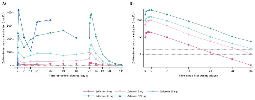
Figure 1: Pharmacokinetics of zalfermin after MADs in healthy male and female participants.
(A) shows the geometric mean for the full concentration–time profiles. (B) shows the geometric mean for concentration–time profiles at steady state and elimination on the logarithmic scale. The dotted lines in both graphs are reference lines for the LLOQ. Values below the LLOQ were imputed. LLOQ, lower limit of quantification; MAD, multiple ascending dose.

Table 3: Pharmacokinetics of zalfermin at steady state after MADs in healthy male and female participants.

	Zalfermin
	3 mg(n = 10)	9 mg(n = 9)	27 mg(n = 9)	60 mg (n = 9)
t1/2,SS, h	122 (23.0)	127 (21.3)	120 (12.6)	122 (5.2)
Cmax,SS, nmol/L	20.4 (24.8)	98.1 (31.4)	162 (23.1)	399 (24.1)
tmax,SS, h	29 (71.9)	38 (41.9)	37 (30.2)	37 (29.3)
CL/FSS, L/h	0.0565 (22.1)	0.0347 (31.9)	0.0599 (25.1)	0.0553 (24.8)

Data are geometric mean (CV). Data are not shown for the 120 mg treatment group as treatment at this dose was discontinued early due to adverse events. CL/F_SS, total apparent serum clearance at steady state; C_max,SS, maximum plasma concentration at steady state; CV, coefficient of variation; MADs, multiple ascending doses; t_1/2,SS, terminal serum half-life at steady state; t_max,SS, time to C_max at steady state.

Pharmacodynamics

Body Weight, Waist Circumference, Whole Body Fat Mass, and Whole Body Lean Mass

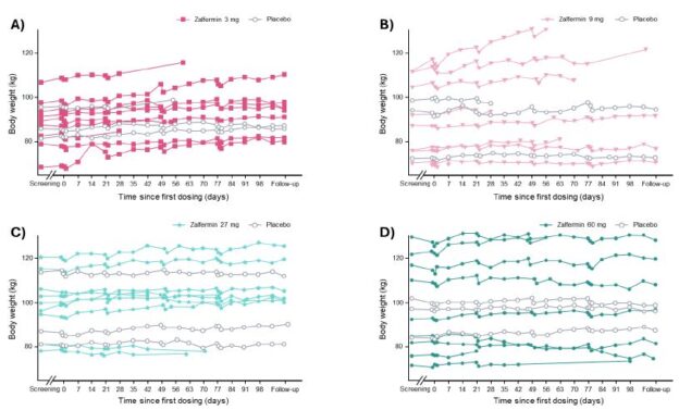
Changes in body weight over time are shown in Figure 2. A statistically significant weight gain of 4.5 %-points (placebo-adjusted) was observed in the zalfermin 3 mg treatment group (P = 0.0008). For the zalfermin 60 mg treatment group, a weight loss of 1.9 %-points was observed; however, this was not statistically significant compared with placebo (Figure S2). No clinically relevant change or dose dependency was observed across any zalfermin dose for waist circumference, whole body fat mass, and whole body lean mass (Figure S2).

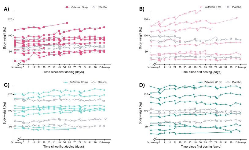
Figure 2: Change in body weight according to zalfermin dose over time: (A) 3 mg, (B) 9 mg, (C) 27 mg, and (D) 60 mg.
Data are not shown for the 120 mg treatment group as treatment at this dose was discontinued early due to adverse events.

Lipids

Sustained improvements in TG, HDL-C, and LDL-C levels were observed at EOT (Figure 3). The change from baseline to EOT in TG and VLDL-C was significant across the zalfermin 3 mg to 60 mg treatment groups versus placebo (P < 0.05) (Figure 4). Improvements in HDL-C and LDL-C were dose dependent, with the greatest improvements achieved with the zalfermin 60 mg dose versus placebo (P = 0.0113 and P = 0.0135, respectively; Figures 3 and 4).  Improvements in TC were significant for the zalfermin 27 and 60 mg doses versus placebo (P = 0.0023 and P = 0.0116, respectively). For beta-hydroxybutyrate, non-significant increases favored zalfermin versus placebo with the exception of the 27 mg dose (Figure 4).

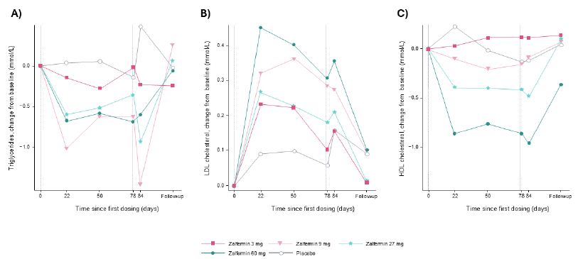
Figure 3: Change from baseline in lipids: (A) triglycerides, (B) LDL cholesterol, and (C) HDL cholesterol after MADs of zalfermin in healthy participants.
Data are not shown for the 120 mg treatment group as treatment at this dose was discontinued early due to adverse events.
Vertical dotted reference lines represent first and last doses of zalfermin.
HDL, high-density lipoprotein; LDL, low-density lipoprotein; MAD, multiple ascending dose.

Placebo-adjusted changes in the 3, 9, 27, and 60 mg treatment groups were −33%, −52%, −61%, and −48%, respectively, for TGs; −1%, −4%, −17%, and −14%, respectively, for TC; 7%, −1%, −13%, and −20%, respectively, for LDL-C; −32%, −52%, −61%, and −48%, respectively, for VLDL-C; 51%, 10%, −26%, and 12%, respectively, for beta-hydroxybutyrate; and −1%, 11%, −1%, and 20%, respectively, for HDL-C (Figure 4).

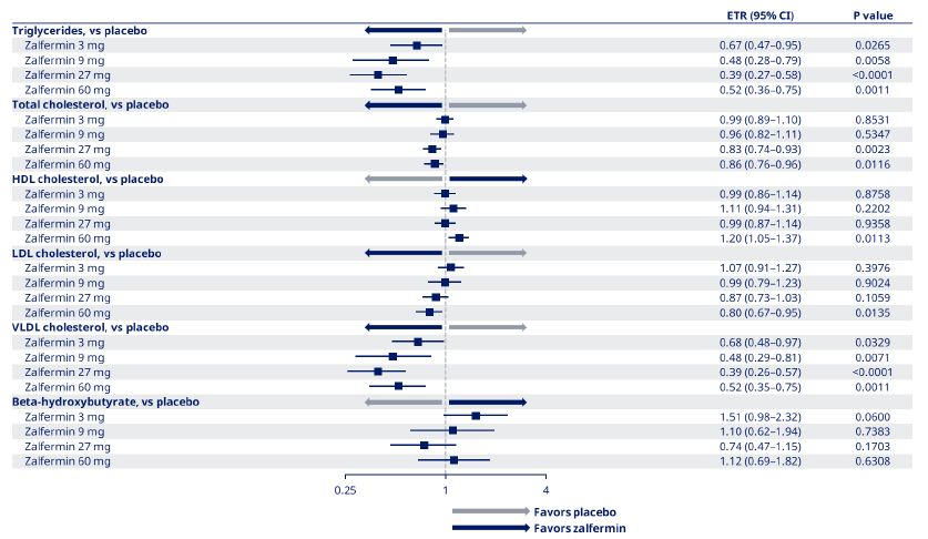
Figure 4: Estimated treatment ratios for change from baseline to end of treatment in lipids for zalfermin versus placebo.
Data are not shown for the 120 mg treatment group as treatment at this dose was discontinued early due to adverse events.
CI, confidence interval; ETR, estimated treatment ratio; HDL, high-density lipoprotein; LDL, low-density lipoprotein; VLDL, very low-density lipoprotein.

Hormones

Decreases in plasma leptin levels were observed at EOT in all zalfermin treatment groups with no clear dose dependency (Table S9). Plasma soluble leptin receptor levels increased across all the zalfermin treatment groups at EOT; changes were not dose dependent (Table S9). The ETRs for plasma leptin and plasma soluble leptin receptor levels across all zalfermin treatment groups are presented in Figure S3. Changes in plasma leptin levels favored zalfermin except for the 3 mg dose (Figure S3). Changes in plasma soluble leptin receptor levels favored zalfermin across all treatment groups (Figure S3).

Glucose Metabolism

Variations in mean glucose metabolism parameters were observed across the zalfermin treatment groups, with no clear dose dependency. No clinically meaningful changes in FSG, FSI, or FPG were observed across the zalfermin treatment groups (Table S10). A reduction in HbA_1c was observed in all zalfermin treatment groups, with greatest reduction observed in the 27 and 60 mg treatment groups (Table S10).

The ETRs for the glucose AUCs were consistently but not statistically significantly slightly above 1 for the 3 mg to 60 mg treatment groups, indicating a minimally higher glucose excursion with the OGTT. This was accompanied by a slight non-significant lowering below 1 in the ETRs for insulin AUCs in the two highest treatment groups (27 and 60 mg) at EOT, compared with baseline. This tendency was not confirmed for the incremental AUCs for insulin and glucose for the highest dose of zalfermin (Table S11).

Discussion

In the current study, AEs were mainly GI related across all MADs of zalfermin and were mild to moderate in severity. Zalfermin was generally well tolerated, except for the 120 mg treatment group that was terminated early due to GI-related AEs (vomiting and nausea). No deaths, serious AEs, or AEs related to technical complaints were reported across any of the zalfermin treatment groups. Overall, zalfermin had a safety profile that was consistent with the FGF21 analog class [13,23-26]. No clinically relevant effect on the menstrual cycle, female reproductive organs, or sex hormones were observed, and no clinically relevant changes at follow-up were observed in other safety parameters. Although slight increases in SBP and DBP were observed in the higher-dose zalfermin treatment groups, these were not regarded as events directly caused by treatment but likely incidental findings. Of note, one other FGF21 analog (PF-05231023) has reported slight increases in blood pressure [27]. Low-titer anti- zalfermin antibodies were detected in 14 participants with no clinical impact. Given that the 120 mg dose in this current study was terminated prematurely, the 60 mg dose appears to be the maximum tolerated dose for weekly administration.

Dose proportionality was observed for AUC_0-168,SS and C_max,SS. The geometric mean t_½,SS of zalfermin ranged from 120 to 127 hours, and t_max,SS ranged from 29 to 38 hours across the zalfermin 3 mg to 60 mg treatment groups. The approximate plasma half-life of zalfermin of 120 hours (5 days) was determined in the SAD study [16] and corroborated in this study. Therefore, zalfermin may be capable of sustained PD activity with a once-weekly dosing regimen. By comparison, other FGF21 analogs such as efruxifermin and pegozafermin have reported half-lives in humans of 3–3.5 days, which were suitable for once-weekly dosing [14,28]. Other PK parameters, for example C_max and t_max, were also similar between this study and the SAD study [16].

Participants in the lower-dose zalfermin treatment groups experienced some weight gain, likely mediated by an increase in appetite and patient-reported changes in food preferences, which has also been described in preclinical species [29,30]. In addition, some other FGF21 analogs have shown an increase in appetite with no clinically meaningful change in body weight [13,31]. In this current study, no clinically meaningful change in body weight was observed in the 60 mg treatment group, where increase in appetite was observed, indicating a potential treatment effect on energy expenditure. By comparison, no clinically meaningful weight loss was observed in the SAD study [16]. In a previous study, efruxifermin did not demonstrate meaningful weight loss at lower doses of 7 and 21 mg compared with the higher doses of 70 and 140 mg [13]. Furthermore, in another study, efruxifermin 50 mg did show a trend toward body weight reduction [32]. Thus, it is likely that studies involving higher doses of zalfermin and of longer duration may be needed for clinically significant weight loss to be observed; however, the effect on body weight reduction would need to be carefully balanced with the observed GI-related AEs. At the time of writing, the phase II study (NCT05016882) of zalfermin 30 mg and semaglutide combination therapy is in progress to determine their effect on MASH resolution and fibrosis improvement in patients with MASH and fibrosis stages 2–4 [33]. Semaglutide has previously demonstrated glucagon-like peptide-1 receptor agonist- mediated weight reduction [34], and it is hypothesized that this would confer additional benefit alongside zalfermin treatment.

Changes in leptin favored zalfermin versus placebo across all doses (except the 3 mg dose) despite no clinically significant weight loss across zalfermin treatment groups. This may be related to the mechanism of action of zalfermin with modulation of adipokines in adipose tissue, resulting in alterations in secretion and systemic leptin sensitivity [35]. A decrease in leptin may also be related to the decrease in female fertility that was observed preclinically [15,17-20], suggesting that this may not translate to patients with overweight/ obesity.

Positive effects on the lipid profile in humans have previously been demonstrated with other FGF21 analogs [13,24-26]. The percentage changes from baseline in TG, HDL-C, LDL-C, and VLDL-C levels for the 60 mg treatment group in this analysis were –48%, 20%, –20%, and –48%, respectively. Specifically for TG and VLDL-C, significant treatment effects were observed across all zalfermin treatment groups versus placebo (3 mg to 60 mg). These results are consistent with the lipid profile improvement reported in the SAD study [16]. Although this study was conducted in healthy volunteers with overweight/ obesity, these results indicate that zalfermin may be promising not only as pharmacotherapy for the treatment of MASH but for other cardiometabolic-related disorders such as dyslipidemia and severe hypertriglyceridemia [36].

No clinically meaningful changes in FSG, FSI, and FPG were observed across the zalfermin treatment groups. This is consistent with the results from the SAD study, where no clinically relevant changes were observed in glucose metabolism parameters [16]. This could be explained by the fact that in both the current study and the SAD study, analyses were conducted in populations without diabetes, and therefore, clinically meaningful changes in glucose metabolism parameters were not expected. However, in this current analysis, reduction of HbA_1c was observed and was greatest in the zalfermin 27 and 60 mg treatment groups. This is likely attributable to the MAD design of this study, with participants having a higher exposure to zalfermin compared with the SAD study [16], and where an effect on HbA_1c was harder to observe with once-weekly single dosing. In addition, participants in this current study had obesity and therefore may also have been insulin resistant. Furthermore, the results of the OGTT, with a slight increase in glucose excursion rate across all doses of zalfermin and a lowering of insulin, could suggest a reduction of glucose tolerance. This finding is not supported by the HbA_1c results where a reduction was observed at the higher zalfermin dose levels. One explanation could be that the relationship observed between zalfermin and glucose tolerance may be influenced by body weight; however, further investigation is needed to assess this.

Some FGF21 analogs have shown sustained effects on insulin sensitivity and trends in the lowering of FPG [13,24]. However, in two previous studies, the results observed were in populations with type 2 diabetes, and therefore, the effects on glycemic parameters may be more pronounced than in the current study [13-24]. Nevertheless, further studies are warranted to determine potential effects of zalfermin on glucose metabolism parameters in participants with types 2 diabetes.

This study had several limitations. Although the purpose of the trial was to primarily assess safety and tolerability to establish a well- tolerated dose range for zalfermin to be investigated in larger trials, the relatively small sample size of 57 participants, and short duration and follow-up time, may affect the generalizability of the safety and efficacy assessments. Furthermore, most of the population was White and no Asian participants were included, thus there was limited diversity in this trial. In addition, fewer females were included in the 27 and 60 mg treatment groups, thus, there are limited data on the effects of zalfermin on the menstrual cycle and reproductive organs at higher doses. Longer, larger clinical studies may provide further insights into the efficacy and safety of zalfermin in more diverse populations.

Based on the safety and PK profile established during this MAD study of subcutaneous zalfermin, the maximum tolerated dose was 60 mg, and this was compatible with a once-weekly dosing regimen. The PD profile of zalfermin, particularly the improvement in the plasma lipid profile, is promising for the treatment of a range of cardiometabolic diseases such as MASH and dyslipidemia. The results obtained from this trial support further clinical development of zalfermin.

Acknowledgments

The authors thank the trial participants, the investigators, and trial site staff who conducted the trial. Medical writing support was provided by Casey McKeown, RVN, FdSc, and Liam Gillies, PhD, of Titan, OPEN Health Communications, and funded by Novo Nordisk, in accordance with Good Publication Practice (GPP) guidelines (www.ismpp.org/gpp-2022).

Data availability Access request proposals can be found at novonordisk-trials.com

Funding

This study was funded by Novo Nordisk A/S.

Conflict of interest disclosure

K.D., J.S.H., M.S.P., S.L.L., O.B., S.T., and B.A. are all employees of and shareholders in Novo Nordisk. C.K. is an employee of and shareholder in ICON.

Ethics approval

The trial was conducted in accordance with the Declaration of Helsinki and Good Clinical Practice guidelines. The protocol for this trial was approved by an independent ethics committee/institutional review board.

Participant consent

All participants provided written informed consent.

Clinical trial registration

This study is registered with ClinicalTrials.gov (NCT03479892).

Author contributions

K.D., J.S.H., M.S.P., S.L.L., O.B., S.T., and B.A. wrote the manuscript; K.D., J.S.H., M.S.P., S.T., and B.A. designed the research for the SAD and MAD studies; K.D., J.S.H., S.T., and B.A. performed the research for the SAD and MAD studies; K.D., J.S.H., M.S.P., S.T., and B.A. analyzed the data; S.L.L. and O.B. contributed new reagents and analytical tools; C.K. was the principal investigator and responsible for assessment of adverse events as well as the medical care of the participants during the study.

References

1. Rinella ME, Lazarus JV, Ratziu V, et (2023) A multisociety Delphi consensus statement on new fatty liver disease nomenclature. J Hepatol. [crossref]
2. Takahashi Y, Fukusato T (2014) Histopathology of nonalcoholic fatty liver disease/ nonalcoholic World J Gastroenterol. [crossref]
3. Chalasani N, Younossi Z, Lavine JE, et al. (2018) The diagnosis and management of nonalcoholic fatty liver disease: Practice guidance from the American Association for the Study of Liver Hepatology. [crossref]
4. Murag S, Ahmed A, Kim D (2021) Recent epidemiology of nonalcoholic fatty liver Gut Liver. [crossref]
5. Younossi ZM, Koenig AB, Abdelatif D, et al. (2016) Global epidemiology of nonalcoholic fatty liver disease:Meta-analytic assessment of prevalence, incidence, and Hepatology. [crossref]
6. Le MH, Yeo YH, Li X, et (2022) 2019 global NAFLD prevalence: a systematic review and meta-analysis. Clin Gastroenterol Hepatol. [crossref]
7. Harrison SA, Bedossa P, Guy CD, et (2024) A phase 3, randomized, controlled trial of resmetirom in NASH with liver fibrosis. N Engl J Med. [crossref]
8. Kharitonenkov A, Shiyanova TL, Koester A, et (2005) FGF-21 as a novel metabolic regulator. J Clin Invest. [crossref]
9. Xu J, Lloyd DJ, Hale C, et (2009) Fibroblast growth factor 21 reverses hepatic steatosis, increases energy expenditure, and improves insulin sensitivity in diet- induced obese mice. Diabetes. [crossref]
10. Xie T, Leung PS (2017) Fibroblast growth factor 21: a regulator of metabolic disease and health span. Am J Physiol Endocrinol Metab. [crossref]
11. Keinicke H, Sun G, Mentzel CMJ, et al. (2020) FGF21 regulates hepatic metabolic pathways to improve steatosis and Endocr Connect. [crossref]
12. Kliewer SA, Mangelsdorf DJ (2019) A dozen years of discovery: insights into the physiology and pharmacology of FGF21. Cell Metab. [crossref]
13. Kaufman A, Abuqayyas L, Denney WS, et al. (2020) AKR-001, an Fc-FGF21 analog, showed sustained pharmacodynamic effects on insulin sensitivity and lipid metabolism in type 2 diabetes Cell Rep Med. [crossref]
14. Rosenstock M, Tseng L, Pierce A, et al. (2023) The novel glycoPEGylated FGF21 analog pegozafermin activates human FGF receptors and improves metabolic and liver outcomes in diabetic monkeys and healthy human volunteers. J Pharmacol Exp Ther. [crossref]
15. Sass-Ørum K, Tagmose TM, Olsen J, et al. (2024) Development of zalfermin, a long- acting proteolytically stabilized FGF21 analog. J Med Chem. [crossref]
16. Dahl K, Hansen JS, Clausen J, et al. (2022) SAT116 – Sustained reduction of triglyceride and LDL cholesterol from single administration of the novel long-acting FGF21 analogue 0499. J Hepatol.
17. Ahart ER, Phillips E, Wolfe MS, Marsh C (2021) The role of kisspeptin in the ovarian cycle, pregnancy, and IntechOpen.
18. Zhang Y, Cao X, Chen L, et al. (2020) Exposure of female mice to perfluorooctanoic acid suppresses hypothalamic kisspeptin-reproductive endocrine system through enhanced hepatic fibroblast growth factor 21 synthesis, leading to ovulation failure and prolonged J Neuroendocrinol. [crossref]
19. Singhal G, Douris N, Fish AJ, et (2016) Fibroblast growth factor 21 has no direct role in regulating fertility in female mice. Mol Metab. [crossref]
20. Owen BM, Bookout AL, Ding X, et al. (2013) FGF21 contributes to neuroendocrine control of female Nat Med. [crossref]
21. S. Food and Drug Administration (2018) Guidance for industry: Bioanalytical method validation.
22. European Medicines Agency, Committee for Medicinal Products for Human Use (CHMP) (2011) Guideline on bioanalytical method validation.
23. Dong JQ, Rossulek M, Somayaji VR, et al. (2015) Pharmacokinetics and pharmacodynamics of PF-05231023, a novel long-acting FGF21 mimetic, in a first- in-human Br J Clin Pharmacol. [crossref]
24. Gaich G, Chien JY, Fu H, et al. (2013) The effects of LY2405319, an FGF21 analog, in obese human subjects with type 2 diabetes. Cell Metab. [crossref]
25. Loomba R, Lawitz EJ, Frias JP, et al. (2023) Safety, pharmacokinetics, and pharmacodynamics of pegozafermin in patients with non-alcoholic steatohepatitis: a randomised, double-blind, placebo-controlled, phase 1b/2a multiple-ascending-dose Lancet Gastroenterol Hepatol. [crossref]
26. Alkhouri N (2022) Pharmacokinetic (PK) and pharmacodynamics (PD) of BIO89- 100, a novel glycoPEGylated FGF21, in non-alcoholic steatohepatitis (NASH) patients with compensated J Hepatol.
27. Kim AM, Somayaji VR, Dong JQ, et al. (2017) Once-weekly administration of a long-acting fibroblast growth factor 21 analogue modulates lipids, bone turnover markers, blood pressure and body weight differently in obese people with hypertriglyceridaemia and in non-human primates. Diabetes Obes Metab. [crossref]
28. Charles ED, Neuschwander-Tetri BA, Frias JP, et (2019) Pegbelfermin (BMS- 986036), PEGylated FGF21, in patients with obesity and type 2 diabetes: results from a randomized phase 2 study. Obesity (Silver Spring) [crossref]
29. Talukdar S, Owen BM, Song P, et (2016) FGF21 regulates sweet and alcohol preference. Cell Metab. [crossref]
30. von Holstein-Rathlou S, BonDurant LD, Peltekian L, et al. (2016) FGF21 mediates endocrine control of simple sugar intake and sweet taste preference by the Cell Metab. [crossref]
31. Loomba R, Sanyal AJ, Kowdley KV, et al. (2023) Randomized, controlled trial of the FGF21 analogue pegozafermin in NASH. N Engl J Med. [crossref]
32. Harrison SA, Frias JP, Neff G, et (2023) Safety and efficacy of once-weekly efruxifermin versus placebo in non-alcoholic steatohepatitis (HARMONY): a multicentre, randomised, double-blind, placebo-controlled, phase 2b trial. Lancet Gastroenterol Hepatol. [crossref]
33. gov (2005) Research study on whether a combination of 2 medicines (NNC0194 0499 and semaglutide) works in people with non-alcoholic steatohepatitis (NASH)
34. Lau DCW, Batterham RL, le Roux CW (2022) Pharmacological profile of once- weekly injectable semaglutide for chronic weight Expert Rev Clin Pharmacol. [crossref]
35. Antonellis PJ, Kharitonenkov A, Adams AC (2014) Physiology and Endocrinology Symposium: FGF21: insights into mechanism of action from preclinical studies. J Anim Sci. [crossref]
36. Bhatt DL, Bays HE, Miller M, et al. (2023) Pegozafermin for the treatment of severe hypertriglyceridemia: a randomized, double-blind, placebo-controlled phase 2 study (ENTRIGUE STUDY) Metab Clin Exp.

References

1. Young EJ (2000) Brucella species. In: Doughlas and Bennett’s Principles and Practice of Infectious Diseases. Mandell GL, Bennett JE, Dolin R (eds) Elsevier Churchill Livingstone, Philadelphia, USA.
2. Alton GG, Forsyth JRL (2004) Brucella, General Concepts. Medical Microbiology, Fourth edition
3. OIE (2009) Bovine Brucellosis: Terrestrial Manual. Office International des Epizooties.
4. Agada CA, Ogugua AJ, Anzaku EJ (2018) Occurrence of brucellosis in small ruminants slaughtered at Lafia Central Abattoir, Nassarawa State, Nigeria. Sokoto J Vet Sci [crossref]
5. Franco MP, Mulder M, Gilman RH, Smits HL (2007) Human brucellosis. Lancet Infect Dis [crossref]
6. CDC (2005) Brucellosis. Centers for Disease Control and Prevention.
7. OIE (2018) Bovine Brucellosis. In: Terrestrial Manual, Chapter 2.4.3. Office International des Epizooties
8. Sofian M, Aghakhani A, Velayati AA, Banifazl M, Eslamifar A, Ramezani A (2008) Risk factors for human brucellosis in Iran: a case-control study. Int J Infect Dis [crossref]
9. Dias RA, Gonçalves VSP, Figueiredo VCF (2009) Epidemiological situation of bovine brucellosis in the State of São Paulo, Brazil. Arq Bras Med Vet Zootec
10. Bronsvoort BM, Koterwas B, Land F, Handel IG, Tucker J, Morgan KL, Tanya VN, Abdoel TH, Smits HL (2009) Comparison of a flow assay for brucellosis antibodies with the reference cELISA test in West African Bos indicus. PLoS One [crossref]
11. Ogugua AJ, Akinseye OV, Ayoola MC, Stack J, Cadmus SIB (2015) Risk factors associated with brucellosis among slaughtered cattle: Epidemiological insight from two metropolitan abattoirs in Southwestern Nigeria. Asian Pac J Trop Dis [crossref]
12. Mubanga M, Mfune RL, Kothowa J, Mohamud AS, Chanda C, Mcgiven J, Bumbangi FN, Hang’ombe BM, Godfroid J, Simuunza M, Muma JB (2021) Brucella seroprevalence and associated risk factors in occupationally exposed humans in selected districts of Southern Province, Zambia. Front Public Health [crossref]
13. Yakubu A, Salako AE, Imumorin IG (2011) Comparative multivariate analysis of biometric traits of West African dwarf and red Sokoto goats. Trop Anim Health Prod [crossref]
Toponym Disputes in Indigenous North America
DOI: 10.31038/GEMS.2025751
Toponyms is a general scholarly study of place names as they have been established and disputed over time by different cultural groups and nation states. Culturally based place names can reference small geosites, long ceremonial landscapes based on established trails, and massive geoscapes that are functionally integrated by geology, climate, and human use. Many of these geosites have been celebrated by nations in recent times as national parks and world heritage sites. Multivocality is a term used by the USA federal government to reflect multiple names for places by cultural groups. Sunset Crater in Arizona after ethnographic studies [1] involving multiple Native groups who are now recognizes in a trail sign containing authentic traditional toponyms reflecting ancient connections with this volcano (Figure 1). Surrounding the park are volcanic lands (Figure 2). The park continues to be referred to by its colonial name Sunset Crater and the surrounding lands are called the Flagstaff Volcanic Landscape.
A geosite is best understood in terms of its surrounding topography (geoscape). A new trail sigh provides a map of eight Native toponyms (Figure 2). Only one mountain toponym is allocated to each tribe or pueblo although all peaks in this area have their own Native names and stories. Note the Native toponyms map is imbedded in a larger colonial toponym interpretation where the peaks are named after one Spanish and three English colonial explorers, and the area is called by the Spanish colonial name, the San Franciso Mountains. Figure 2B illustrates the complexity of modern toponym renaming and the resulting multivocality.
Figure 1: The multivocality of cultural place names on a trail sign at Sunset Crater National Monument in Arizona (soured Van Vlack 2025) [2].
As they increasingly become more formally defined and celebrated, debates over place names and their meanings have increased, which, now have been more specifically defined by Toponymic Guidelines of the United Nation which have been negotiated by a series of formal committees (United Nations Group of Experts on Geographical Names2018) [3]. The content of Toponymic Guidelines has been developed since 1979 and includes information about official, national and minority languages, names authorities, source material for toponyms, glossaries, abbreviations used on official maps, differentiating text from toponyms on national maps, and administrative regions. At the Ninth Conference (United Nations 2007) [4], it was acknowledged that the format should not be too restrictive; also considered important were having guidelines in more than one language and cooperating with neighboring countries. A toponymic landscape involves the functional interconnections of geosites and geotrails to form a geoscape. The naming of new places during colonial expansion is well documented. For example, in Australia, studies analyze the effects of British settler colonialism on the toponymic landscape of lands traditionally cared for by Indigenous Australian peoples [5]. So, in the Australian research and analysis as of contemporary national efforts to rectify these past colonial changes. Detailed toponymic research has focused on lands where Germans were the first settler colonialists to alienate land in portions of southern Australia, thus dispossessing the Nunga as traditional owners. The encroaching German settlers created a toponymic landscape that reflected their culture and history and the geological characterizes of the new lands where they settled. The German toponymic landscape of settled places was derived from religious sources, from a person’s name, and from the name of their home communities in German.
Figure 2: A Park Trail Sign Identify Nearby Native Toponyms of Volcanic Mountains (Source Van Vlack 2025) [2].
The Cases
This brief, case-based review essay reflects findings from five of our ethnographic studies that have involved Native Americans. Each case illustrated contemporary Toponyms issues involving Native people and Colonial Settlers in North America and disputes over the names of places. Each of these case studies represent but a small segment of a much broader international issue that was largely crated by worldwide human events in the Pre-colonial, Colonial, Post-colonial, and Neocolonial periods which have occurred over the past 500 years. All these cases of Toponym disputes have occurred or are occurring between the Native and Colonial peoples. The cases involve Geosites, Geotrails, and Geoscapes. Findings from all cases are available publicly.
Geosite- Mato Tepe or Devils Tower, Wyoming
Mateo Tepe (Figure 3) is a Native name for a shared sacred geosite composed earth and fire materials. Debate of toponyms is whether it should be the stairs to Heaven as the 23 Native tribes maintain or the steps to Hell as the Devils Tower implies (Stoffie et al 2024). This place name debate immediately when it was mapped by exploring expedition of the USA colonial state and continues to today. Mateo Tepe has been placed on the list of the most important geosites in the World and was nominated as both a geology place and a cultural place [6]. Using both Toponyms, this geosite was awarded a position on the official lists of significant International Commission on Geoheritage Sites.
Figure 3: Mateo Tepe Stairs to Heaven or Steps to Hell?
Devils Tower was declared as the first National Monument because of its geological value, but it is now recognized for its value for Native Americans.
Geotrail – Old Spanish Trail: Native Communities, USA Southwest
The Old Spanish Trail (OST) has been designated as a National Historic Trail by the NSP. An ethnographic study [7] involving Native tribes who traditionally lived along the trail study was funded and thus were impacted by the thousands of animals and people who traveled in large caravans along it from New Mexico to California. All participating tribes disputed the US applied name for the trail which they maintained was a series of traditional Native trails linked for the caravans. The Taos Pueblo was so incensed by the name that they refused to participate in the study even though the events along the OST were key in their history.
Geoscape – Bears Ears, Utah
Presently 32 tribes have expressed cultural connections to Bears Ears (Figure 4) as a geosite and its surrounding geoscape. Each tribe has a name for this place in their own language and their own stories about why it is important. The Hopi refer to it as Hoon’Naqvut, the Navajo call it Shash Jaa,’ the Utes named it Kwiyagatu Nukavachi, and for Zuni it is Ansh An Lashokdiwe. During an ethnographic study that involved nine culturally affiliated tribes, tribal representatives shared their deep time but different kinds of cultural attachments to this geosite and geoscape [2].
Figure 4: Bears Ears is a culturally significant geoscape in southeast Utah.
Geoscape – Iliamna Lake (Nanvarpak, Nila Vena) Native and Local Place Names Alaska)
This is an extended ethnographic and linguistic study of a Native toponyms associated with large lake (Figure 5) (a geosite) and the numerous geosites that constitute its massive integrated surrounding geoscape [8-10]. The research illustrates how difficult it is to both explain and share toponymic information across linguistic and cultural differences. The researcher devoted years to accomplishing this goal which had epistemological, cultural protocols, and privacy challenges.
Figure 5: Iliamna Lake, Biggest Lake in Alaska.
Geoscape – El Malpais National Monument, New Mexico
El Malpais National Monument is an ancient area consisting of two unique geoscapes– lava flows occurring on top of each other forming layers of volcanic fields (Figure 6) and underground lava tunnels (Figure 7). It occurs at the foot of a massive sacred mountain with the colonial name Mount Taylor. The mountain and lava field are active ceremonial areas and considered living due to the rebirth of the Earth.
Figure 6: Volcanic Fields of El Malpais National Monument.
Today the lava flows are managed as a park by the US NPS using the area’s original colonial toponym. El Malpais is a Spanish term for a bad place or bad lands but the many tribes and pueblos who participated in the NPS funded ethnographic study of this lava flow park define it using their own linguistic terms and traditional uses patterns that its cultural importance and spiritual value [11].
Figure 7: One of Many Lava Tunnels in the Monument.
Toponyms Discussion
Many geosite toponym disputes are between Native people whose lands are involved in encroachment of members of the conquering colonial society. Native people today, however, often experience conflict with each other regarding appropriate place terms. This is a situation debate that derives from the western views of property and ownership of places. A finding from our ethnographic studies is that places are culturally layered with different meaning specific to the peoples who have interrelated with each other and the geosite for long periods. For Native people of the Southwest US this is now documented to be about 40,000 years. Deep time and multicultural connections make for complex understandings of places, as our studies have shown. This complexity becomes a key issue when Native people participate as tribal representatives at land management meetings where their desire to apply or preference traditional toponyms face resistant from supporters of colonial toponym meanings.
1. Stoffie, Richard, and Kathleen Van Vlack (2022) Talking with a Volcano: Native American Perspectives on the Eruption of Sunset Crater, Arizona. Land 11.
2. Van Vlack Kathleen, H Lim, J Yaquinto, J Gazing Wolf, B Eguino-Uribe, et (2025) Monticello BLM Ethnographic Partnership: An Ethnographic Overview and Assessment of the Cedar Mesa and Bears Ears Region. Heritage Lands Collective: Cortez, CO.
3. United Nations Group of Experts on Geographic Names (2018) Toponymic Guidelines for Map and Other Editors for International Use.
4. United Nations (2007) Ninth United Nations Conference on the Standardization of Geographical New York. United Nations.
5. Spennemann DHR (2025) A Disappearing Cultural Landscape: The Heritage of German-Style Land Use and Pug-And-Pine Architecture in Land. 14.
6. Stoffie R, K Van Vlack V, Semeniuk, M Brocx (2025) Devils Tower, Mateo The Second 100 IUGS Geological Heritage Site. The Second 100 IUGS Geological Heritage Site.
7. Stoffie R, K Van Vlack R, Toupal S, O’Meara, R Arnold (2008) American Indians and the Old Spanish Tucson, AZ: Bureau of Applied Research in Anthropology, University of Arizona.
8. Kugo Y (2020) Artic Data: Iliamna Lake (Nanvarpak, Nila Vena) Native and Local Place Names (2016-2019).
9. Kugo Y (2021) Documenting Yup’ik Place Names with Yoko Kugo. Artic Data Center Blog.
10. Kugo Y( ed) (2024) Nanvarpagmiut Qanemciit-llu/ Iliamna Lake People and Their Stories: Place Names and Sense of Fairbanks, AK: Alaska Native Language Center, University of Alaska.
11. Larsson Simon (2025) The Connectedness of People and Geological Features in the El Malpais Lava Flows of New Mexico, USA. Land 14.
Use of Preoperative Low Dose Etomidate Infusion in Severe Ectopic ACTH-Dependent Cushing Syndrome Due to Thymic Carcinoid: A Case Report
1. Thomas R (2025a) The change from the supercritical fluid-melt system into the under-critical stage: The Zinnwald example. Geol Earth Mar Sci 7: 1-9.
2. Thomas R, Trinkler M (2024) Monocrystalline lonsdaleite in REE-rich fluorite from Sadisdorf and Zinnwald/E-Erzgebirge, Germany. Geol Earth Mar Sci 6: 1-5.
3. Bauer W (2013) Gusseisen mit Lamellengraphit, Leoben, ÖGI-Eigenverlag.I-V and 95 PG.
4. Keller DS, Ague JJ (2022) Possibilities for misidentification of natural diamond and coesite in metamorphic Neues Jb. Mineral Abh 197: 253-261.
5. Thomas R, Davidson P, Rericha A, Recknagel U (2023) Ultrahigh-pressure mineral inclusions in a crustal granite: Evidence for a novel transcrustal transport mechanism. Geosciences 13: 1-13.
6. Hurai V, Huraiová M, Slobodník M, Thomas R (2015) Geofluids – Developments in Microthermometry, Spectroscopy, Thermodynamics, and Stable Isotopes. Elsevier.
7. Lafuente B, Downs RT, Yang H, Stone N (2015) The power of database: the RRUFF project. In: Armbruster T, Danisi, R.M. (eds). Highlights in mineralogical W. De Gruyter, Berlin. Pg: 1-30.
8. Liu Q, Miao H, Liu W, Bu L, Yao J, et (2024) Selective transformation of cementite: Graphitization or spheroidization. Materials Today. 18 pages, under review.
9. Estandia B, Rodriguez L, Alvarez, JA, Ferreño D, Hernández D, et al. (2014) Raman spectroscopy of flake graphite as a tool to detect stress-strain states in cast Advanced Sustainable Foundry. 71st World Foundry Congress in Bilbao. 6 pages.
10. Yang H-P, Wen H-H, Zhao Z-W, Li S-L (2001) Possible superconductivity at 37 K in graphite-sulphur Chin Phys Lett 18: 1648-1650.
11. Thomas R, Rericha A, Pohl WL, Davidson P (2018) Genetic significance of the 867 cm-1 out-of-plane Raman mode in graphite associated with V-bearing green Mineralogy and Petrology 112: 613-645.
12. Gong Y, Luo D, Choe M, Seong WK, Bakharev P, et (2024) Growth of diamond inliquid metal at 1 atm pressure. Nature 629: 348-354.
13. Zaitsev AM (2001) Optical Properties of A Data Handbook. Springer, I-XI, and 1-502 pages.
14. Thomas R (2025b) Strong Isotope Fractionation Between 13C and 12Cin the Supercritical Fluids Related to the Variscan Mineralizations in Erzgebirge, Slavkovský Les (Kaiserwald), and Lusatian Mountains, Germany, and the Czech Republic, and Some Remarks on the Low-Pressure Formation of Geol Earth Mar Sci 7: 1-6.
15. Stefanescu DM, Alonso G, Suarez R (2020)Recent Developments in Understanding Nucleation and Crystallization of Spheroidal Graphite in Iron-Carbon-Silicon Metals 10 Bericht-Nr. 221.
16. Sommerfeld A, Tonn B (2008) Nucleation of graphite in cast iron melts depending on manganese, sulphur, and oxygen. International Journal of Cast Metals Research 21: 23-26.
17. Zykova A, Lychagin, D, Chumaevsky, A, Popova N, Kurzina (2018) Influence of Ultrafine Particles on Structure, Mechanical Properties, and Strengthening of Ductile Cast Iron. Metals.
18. Nandori G, Dul J (1982) Beurteilung von Gußeisenschmelzen durch Messung der Makrovolumenänderungen und der Ausdehnungskräfte während der Erstarrung. Giesserei-Rundschau 29: 9-16.
19. Matjuschkin V, Woodland Ab, Frost DJ, Yaxley M (2020) Reduced methanebearing fluids as a source for diamond. Scientific Peports. 10: 6961, 8 pages.
Review: Knowledge and Prevalence of Cervical Cancer Screening Among Women Receiving Prenatal Care in Accra, Ghana
DOI: 10.31038/IGOJ.2025812
Study Overview
This cross-sectional study examined cervical cancer screening (CCS) knowledge and prevalence among 393 women receiving prenatal care at three health facilities in the Okaikwei North Municipal Assembly, Greater Accra Region, Ghana. Utilizing a two-stage cluster sampling method, the research targeted women over 18 years attending Achimota Hospital (36.6%), Lapaz Community Hospital (32.1%), and NK-Salem Medical Centre (31.3%). The study addressed a critical gap in understanding CCS awareness among pregnant women, a high-risk population with frequent healthcare contact opportunities. The research employed a quantitative methodology with data collection through REDCap electronic surveys administered in English and Asante Twi. Knowledge of CCS was assessed using 12 questions scored from 0-12, with participants categorized into low (0-4), moderate (5-8), and high (9-12) knowledge levels using percentile-based classification. Analysis of covariance (ANCOVA) was used to compare CCS knowledge scores across facilities while controlling for demographic variables including age, marital status, education, employment, and income.
Key Findings
The study revealed alarmingly low levels of both CCS knowledge and screening prevalence. Only 19.8% of participants demonstrated high CCS knowledge, with the majority (98.5%) scoring below adequate levels. The overall mean CCS knowledge score was 3.0 ± 2.57 out of 12 possible points. While 75.6% had heard of CC and 68.4% were aware of CCS, substantial knowledge gaps existed when probed further, thus 46.5% did not understand what CCS entailed, 71.7% were unaware of screening intervals, 62.0% did not know the recommended screening age, and only 33.9% correctly identified Pap smear as the primary screening test. The prevalence of CCS was remarkably low at 7.4%, with 90% of participants never having been screened. This finding aligns with Ghana’s national CCS rates of 2-3% and reflects broader challenges in sub-Saharan Africa where over 85% of global cervical cancer cases occur. Participants correctly identified key risk factors including multiple sexual partners (23.3%), STI infections (18.0%), and early sexual onset (13.1%).
Significance and Inter-facility Variations
A significant finding was the substantial variation in CCS knowledge across health facilities. ANCOVA results revealed statistically significant differences (F (2,384)=75.03, p<0.001, ηp²=0.281), with facility type accounting for 28.1% of variance in knowledge scores beyond demographic factors. Pairwise comparisons showed that women at Achimota Hospital (M=4.33) and NK-Salem Medical Centre (M=4.74) had significantly higher knowledge scores compared to Lapaz Community Hospital (M=1.25). These differences raise facility-specific factors such as patient education programs, healthcare provider engagement, or access to health information materials may influence knowledge levels.
Among demographic covariates, income (ηp²=0.187) and marital status (ηp²=0.144) had the strongest influence on CCS knowledge, followed by age and education. This indicates that financial stability and spousal support may positively affect CCS awareness, while younger, less-educated, and lower-income women face greater knowledge barriers.
Limitations and Methodological Considerations
The study acknowledges several limitations that affect generalizability. The single-district focus in Greater Accra may not represent all Ghanaian women receiving prenatal care, particularly those in rural areas or different socioeconomic contexts. The two-stage cluster sampling method, while enhancing representativeness within the district, may introduce selection bias if certain clusters are more likely to be selected. Additionally, reliance on self-reported data introduces potential recall and social desirability biases.
The cross-sectional design prevents assessment of knowledge changes over time, and the focus on prenatal care attendees may not reflect the general population’s CCS knowledge. The study’s strength lies in its robust sample size (92.9% response rate), rigorous statistical analysis controlling for demographic confounders, and focus on a high-risk population with regular healthcare contact opportunities.
Implications and Future Directions
The findings reveal critical gaps in CCS knowledge and uptake that require urgent intervention. The significant inter-facility differences suggest that targeted, facility-specific interventions may be more effective than uniform approaches. The research recommends integrating structured cervical cancer education into routine prenatal care through health talks, standardized materials in local languages, and most importantly pre- and post-natal counseling sessions.
Practical interventions should include mobile screening clinics, community health worker outreach, and culturally appropriate educational materials. Catering for groups that are characterized by no formal education and unstable financial stability, the employment of existing social networks such as market associations, church groups, neighborhood committees could benefit from CCS education and mobile screenings. The study emphasizes leveraging social media and local dialects for awareness campaigns, as participants identified social media as their primary information source (31.0%). Future research should conduct multi-site studies across different geographical areas/regions to examine disparities among the geographical areas to understand the specific barriers that exist to screening uptake.
Conclusion
This study provides compelling evidence of the urgent need to strengthen cervical cancer prevention efforts in Ghana’s prenatal care settings. The combination of low CCS knowledge levels (19.8% high knowledge) and minimal screening prevalence (7.4%) among pregnant women represents a missed opportunity for early detection and prevention. The significant facility-based variations in CCS knowledge calls for targeted interventions considering the local contexts and demographic factors. Implementing these interventions could substantially improve outcomes. As prenatal care provides a structured platform for health education, integrating comprehensive CCS awareness programs could dramatically enhance early detection rates and reduce cervical cancer mortality in Ghana. The research contributes essential insights for developing evidence-based interventions that address both knowledge gaps and systemic barriers to screening access.
Continuous Glucose Monitoring in Hospitalized Patients: Is It Time to Embrace a Paradigm Shift?
DOI: 10.31038/EDMJ.2025934
The use of continuous glucose monitoring (CGM) has transformed outpatient diabetes care, yet its implementation in the inpatient setting remains limited [1,2]. In our recent systematic review and meta-analysis of six randomized controlled trials (RCTs) (n=979), we evaluated whether adding unblinded CGM (real-time or intermittently scanned) to point-of-care (POC) glucose testing, to assist with insulin adjustment, improves outcomes for non-critically ill, hospitalized adults with diabetes mellitus. We found that the addition of CGM significantly increased time in range (TIR, 70–180 mg/dL) by a mean difference (MD) of +7.24% (P <0.00001), supported by high-certainty evidence. It also reduced time below range (TBR) <70 mg/dL (MD: −1.23%, P=0.02; moderate certainty) and <54 mg/dL (MD: −0.95%, P<0.00001; high certainty). Time above range (TAR) >250 mg/dL decreased by −3.70% (P=0.003), and mean glucose levels declined by −10.93 mg/dL (P=0.0003), both with high-certainty evidence. In terms of safety outcomes, CGM use reduced hypoglycemic events <70 mg/dL (MD: −1.21 events per patient, P=0.001; low certainty) and <54 mg/dL (MD: −1.24 events per patient, P=0.03). Notably, nocturnal hypoglycemic events were also reduced for both <70 mg/dL (MD: −0.16 events per patient, P=0.002) and <54 mg/dL (MD: −0.11 events per patient, P=0.006), although the certainty of evidence was not formally graded for these specific outcomes [1-3].
We believe these findings mark an inflection point in hospital glucose management. While point-of-care (POC) glucose testing has long been the mainstay, CGM offers high frequency of data points, rate-of-change of glycemia over time, direction of blood glucose levels and potential for proactive hypo-and hyperglycemia prevention [4]. Although the six included RCTs in our review varied in population, diabetes types, insulin protocols, and device models (Dexcom G6 and Guardian Sensor 3), our sensitivity analyses demonstrated robust, consistent benefit across subgroups. Nevertheless, we recognize that further research is warranted to address remaining knowledge gaps and to further validate these findings across diverse clinical settings. The implementation of CGM in the general ward still faces several challenges. It requires integration of CGM with electronic medical records and training staff and providers on initiation of download and interpretation. Ideally software integration should include the use of artificial intelligence to pick up patterns of hypo and hyperglycemia and a new “glucose monitoring team,” like a telemetry unit should review those flags in real time and inform the treatment team to make clinical decisions. But even more basic integration can provide retrospective data that will assist providers in making insulin adjustments based on better quality of that than what is provided by POC glucose alone [5].
The 2025 Standards of Care in Diabetes from the American Diabetes Association (ADA) now endorse universal use of CGM for all patients with diabetes, regardless of insulin therapy, as well as the continued use of CGM during hospitalization in those already utilizing the technology [6]. Our findings reinforce this recommendation to continue CGM during hospitalization in patients admitted already using the technology but also as a primary tool that could be started in hospital to assist glycemic management in patients with hyperglycemia. With evidence mounting improved outcomes, fewer hypoglycemic events, and no apparent safety concerns, we believe CGM will eventually be implemented as standard practice for most non-ICU inpatients with hyperglycemia.
In conclusion, continuous glucose monitoring (CGM) represents a significant advancement in diabetes management in non-critically ill hospitalized patients. By enabling continuous insight into glycemic patterns, it facilitates optimized glycemic management, resulting in improved safety and clinical outcomes compared to the use of POC glucose testing alone. With supportive policies, appropriate infrastructure, and comprehensive training, CGM integration into routine inpatient care is warranted – particularly for patients at the highest risk of hypoglycemia. Advancing beyond intermittent glucose measurements to leverage continuous data represents a critical evolution in optimizing inpatient glycemic management.
1. American Diabetes Association Professional Practice Committee (2025) Diabetes Technology: Standards of Care in Diabetes-2025. Diabetes Care. [crossref]
2. Zelada H, Perez-Guzman MC, Chernavvsky DR, Galindo RJ (2023) Continuous glucose monitoring for inpatient diabetes management: an update on current evidence and practice. Endocr Connect. [crossref]
3. Cavalcante Lima Chagas G, Teixeira L, Clemente MRC, et al. (2025) Use of continuous glucose monitoring and point-of-care glucose testing in hospitalized patients with diabetes mellitus in non-intensive care unit settings: A systematic review and meta- analysis of randomized controlled trials. Diabetes Res Clin Pract. [crossref]
4. Agarwal S, Galindo RJ, Shah AV, Abreu M (2024) Diabetes Technology in People with Type 2 Diabetes: Novel Curr Diab Rep. [crossref]
5. Tian T, Aaron RE, Yeung AM, et al. (2023) Use of Continuous Glucose Monitors in the Hospital: The Diabetes Technology Society Hospital Meeting Report J Diabetes Sci Technol. [crossref]
6. American Diabetes Association Professional Practice Committee (2025) Diabetes Care in the Hospital: Standards of Care in Diabetes-2025. Diabetes Care. [crossref]
Safety, Tolerability, Pharmacokinetics, and Pharmacodynamics of the Novel Long-Acting FGF21 Analog Zalfermin: A Multiple Ascending Dose Study in Healthy Participants with Overweight/Obesity
1. Tracy SK (2025) Serial killing: A psychological Cognella (in press).
2. Cullen E (2020) American evil: The psychology of serial killers. Waterside Press.
3. S. Department of Justice, Morton, R. J., Tillman, J. M., & Gaines, S. J (2019) Serial murder: Pathways for investigation. AbeBooks.
4. Ramsland K (2006) Inside the minds of serial killers: Why they Praeger.
5. Sterling E (2019) Desperate motives for murder: Mercenary female baby killers in Victorian England. The Lincoln Humanities Journal, 7(1), 136-153. Available from: https://www.lincoln.edu/_files/academics/Lincoln-Humanities-Journal-Vol-7-2019. pdf#page=137
6. Schechter H (2003) The serial killer files: The who, what, where, how, and why of the world’s most terrifying murders. Ballantine Books.
7. Benkart E (2019) The patterns of women serial killers in a climate of changing gender norms. OSF Preprints. Center for Open Science. Available from: https://doi. org/10.31219/osf.io/pcqk6
8. Wilkins MP (2004) A comfortable evil: Female serial murders in American culture [Doctoral dissertation, Pennsylvania State University]. Electronic Theses and Dissertations for Graduate School.Available from: https://etda.libraries.psu.edu/ catalog/6451
Attachment and Trauma in Therapy: A Neuroaffective Developmental Perspective
DOI: 10.31038/PSYJ.2025731
1. Hart S, Bentzen M (2012) Through Windows of Karnac.
2. Teicher MH, Samson JA, Anderson CM,Ohashi K (2016) The effects of childhood maltreatment on brain structure, function and connectivity. Nature Reviews Neuroscience, 17: 652–666. [crossref]
3. Perry BD (2009) Examining child maltreatment through a neurodevelopmental lens: Clinical applications of the Neurosequential Model of Journal of Loss and Trauma, 14: 240-255.
4. Perry BD, Szalavitz M (2006) The Boy Who Was Raised as a Dog: And Other Stories from a Child Psychiatrist’s Notebook – What Traumatized Children Can Teach Us About Loss, Love, and Basic Books
5. Tronick E,Gianino A (1986) Interactive mismatch and repair: Challenges to the coping Social Perception in Infants.
6. Bentzen M (2021) The Neuroaffective Picture North Atlantic Books.
7. Kearney BE, Lanius RA (2022) The brain-body disconnect: A somatic sensory basis for trauma-related disorders. Frontiers in Neuroscience. [crossref]
8. Porges S (2011) The Polyvagal Norton Books.
9. Schore AN (2003) Affect Dysregulation and Disorders of the Norton Books.
10. Siegel D (2012) The Developing Mind (2nd ) Guilford Books.