DOI: 10.31038/GEMS.2025773

Abstract

Laboratory experiments with rock samples show that creep at small strains is transient and is described by the linear hereditary rheological model of Andrade. Flows that restore isostasy (in particular, postglacial ones) cause deformations in the lithosphere that do not exceed 10^-3 and, therefore, demonstrate transient creep. The effective viscosity characterizing transient creep is lower than the effective viscosity at steady-state creep and depends on the characteristic time of the process under consideration. The characteristic duration of isostatic equilibrium recovery after the initial disturbance of the Earth’s surface relief does not exceed ten thousand years, and therefore the depth distribution of rheological properties differs from the distribution that corresponds to slow geological processes. The perturbations of the Earth’s surface relief caused by an initial small-scale perturbation that disrupts isostasy are considered. The propagation of vertical displacements along the Earth’s surface from the area of the initial perturbation is carried out by diffusion-type waves that arise during the process of isostasy recovery, and by convective waves that arise due to the vertical temperature gradient in the lithosphere. The solutions of the equations of continuum mechanics are obtained using the Fourier transform in the spatial horizontal coordinate and the Laplace transform in time.

Keywords

Transient creep, Isostatic recovery, Vertical movements of the Earth’s surface, Thermoconvective waves, Diffusion-type waves

Introduction

Andrade proposed a law to describe the transient creep he observed experimentally in 1910. This law was later confirmed in numerous laboratory studies of rock creep conducted at high temperatures and pressures typical of the Earth’s interior [1-5]. The well-known concept in mechanics that creep is transient at small deformations was first introduced into geophysics in the work of [6], where the idea was put forward that flows in the mantle associated with small deformations, and, in particular, postglacial flows, occur in the transient creep regime. The concept of transient creep at small deformations of geomaterial was further developed in the monograph [7]. Experimental and theoretical justifications for the applicability of the Andrade rheological model in studying dynamic processes in the lithosphere and mantle are presented in [8]. The lithospheric plate is a cold boundary layer formed by mantle convection, and the thickness of continental plates beneath cratons can exceed 200 km. The rheological model of a power-law non-Newtonian fluid, which describes steady-state creep and is commonly used in modern geophysical studies, leads to a very high effective viscosity characterizing creep at small deformations. With such a high effective viscosity, the lithosphere would be purely elastic even over geological times. Transient creep corresponds to a much lower effective viscosity than steady-state creep. Therefore, transient creep must be taken into account when examining geophysical processes in the lithosphere. The effective viscosity corresponding to transient creep depends on the characteristic duration of the geophysical process under consideration. In [8-11], low-amplitude thermoconvective waves in the lithosphere, the existence of which is due to transient creep, were considered, and it was shown that thermoconvective oscillations (standing waves) lead to the formation of sedimentary basins on continental cratons. The characteristic time of this process is about 108 years. The work [12] considers the recovery of isostatic equilibrium after an initial small – scale disturbance of the earth’s surface relief. As a result of the recovery process, the Earth’s surface returns to a flat position, which corresponds to the equilibrium state with a uniform horizontal density distribution. The characteristic duration of this process does not exceed 1000 years, and therefore the distribution of rheological properties by the depth of the lithosphere and crust differs from the distribution that corresponds to slower processes associated with convective motion. A process with a characteristic time of about 1000 years is a fairly fast process, the study of which does not require taking into account the influence of the vertical temperature gradient present in the lithosphere, since thermal effects are associated with very slowly occurring thermal conductivity. However, this process is slow enough to neglect the elasticity, compressibility, and inertia of the lithosphere.

In this paper, we will consider the movements of the Earth’s surface caused by initial vertical displacements. If a vertical displacement disrupting the isostatic equilibrium of the crust has occurred in some area of the Earth’s surface, then the process of isostasy recovery is reduced not only to a gradual decrease in the initial vertical displacements in this area, but also to the propagation of displacements beyond its boundaries. The processes of displacement propagation in the crust can be called diffusion-type waves. Waves of this type appear when solving parabolic equations of the theory of diffusion or heat conduction. These waves describe the process of propagation of temperature disturbance from the area where the disturbance occurred to the environment. The temperature gradually increases in remote areas, and the temperature in the initially disturbed area decreases. The propagation of the disturbance is accompanied by its strong attenuation, and over time, the temperature disturbance disappears everywhere. This is exactly how the process of displacement propagation occurs in the elastic crust, where the displacement acts as an analogue of temperature disturbance. It will be shown what movements of the Earth’s surface created by diffusion-type and thermoconvective waves caused by the initial vertical displacement of this surface.

Rheological Model

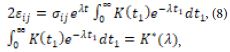
Laboratory studies show that at small deformations transient creep occurs, in which creep deformations depend linearly on the applied constant stresses

where  f(t) is the creep function, which provides an analytical description of transient creep, ε_ij and  is the strain tensor measured from the state at the moment of stress application. For rocks, the creep function at high temperatures is well described by Andrade’s law

where A is the Andrade rheological parameter. At short times, transient creep obeys Lomnitz’s law, but already at times of the order of a day, Andrade’s law becomes valid [13]. Therefore, Andrade’s law will be used in the study of low-frequency waves. The attenuation of high-frequency seismic waves is described by Lomnitz’s rheology [14], but in this paper, although we will talk about Rayleigh surface elastic waves, their attenuation will not be considered. To generalize the results of experiments carried out at constant stresses to the case of variable stresses, we can use the linear Boltzmann theory, valid for sufficiently small deformations. This theory leads to an integral relationship between strains and stresses

where t is the observation time, and K(t) is the integral creep kernel determined by the creep function

As follows from (2) and (4), the creep kernel corresponding to Andrade’s law has the form

The rheological model described by equations (3) and (5) will be called the Andrade model. This model generalizes Andrade’s law to the case of variable stresses. At sufficiently large deformations, transient creep is replaced by steady-state creep, which is described by the rheological model of a power-law non-Newtonian fluid. The value of the Andrade rheological parameter depends on temperature, pressure, and mineralogical composition. The depth distribution of the Andrade parameter was obtained in [11]. Since the Andrade parameter decreases with increasing temperature, and the temperature increases with depth in the lithosphere, this parameter decreases with depth. In the upper crust, the thickness of which is about 20 km, the value of this parameter is estimated as A ≈ 10¹⁶ Pa∗ s^1/3 . With such a high value of  A, the upper crust behaves as an elastic layer even on times of the order of the age of the Earth. More precisely, the upper crust, the thickness of which is about 20 km, is brittle-elastic, and elasticity dominates only in the lower layer of the upper crust, the thickness of which is about 10 km. In the uppermost layer of the crust, brittleness dominates, and its strength is very low [11]. We will assume that the upper crust with a thickness of 20 km is an elastic layer with a reduced shear modulus due to brittleness. Within the framework of the simplified model of the lithosphere beneath the upper crust used in the paper,we use the depth-averaged estimate A ≈ 10¹² Pa∗ s^1/3.

Since the total deviatoric deformation of the medium can be represented as the sum of the deviatoric creep deformation (1) and the deviatoric elastic deformation

where μ is the elastic shear modulus, an elastic-creeping medium whose creep is transient is described by the equation

In linear stability theory, it is assumed that the strains and stresses depend on time as exp(λt), where λ is the complex decrement, and the right-hand side of equation (3) takes the form

where the asterisk denotes the Laplace transform, which is used here only to evaluate the integral in equation (8). The Laplace transform of the creep kernel (5) yields

where the gamma function is Γ (1/3)≈3. Linear stability theory considers the behavior of a mechanical system at large times elapsed since the occurrence of a small disturbance. Therefore, in equation (8), the upper limit of integration is t=∞.

Thus, when the time dependence has the form exp(λt), at large times the effective shear modulus of the Andrade medium has the form

and the effective Newtonian viscosity is written as

where  is the characteristic time of the process. As follows from (11), on time scales of the order of 1000 years, small-scale postglacial flows, which are characterized by an average value of the rheological parameter A ≈ 10¹² Pa∗ s^1/3, correspond to an effective viscosity ℑ_eff ≈ 10¹⁹ Pa∗ s. Such estimate agrees in order of magnitude with the viscosity estimates found when considering small – scale postglacial flows within the framework of the rheological model of a Newtonian fluid [15]. Consequently, the estimates of Andrade parameter obtained on the basis of data from laboratory experiments with rock samples at temperatures and pressures characteristic of the Earth’s interior [11], correspond to the observational data used to estimate the viscosity of the upper mantle [15]. The effective viscosity for the Andrade medium depends on the characteristic time of the process under consideration and, therefore, the effective viscosity found for postglacial flows with a characteristic time of 1000 years cannot be used in the study of slower geological processes [8,13].

Thermoconvective and Elastic Surface Waves

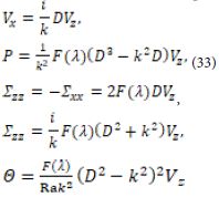
We consider an elastic thin plate lying on a layer with Andrade rheology. The origin of coordinate is placed on the upper surface, and the z-axis is directed vertically upward. The thin plate (z = 0) models the upper elastic crust, and the layer (-1 < z < 0) – the underlying lithosphere. The equations describing the disturbances of the lithostatic equilibrium of an incompressible medium are written as

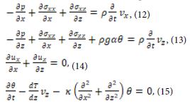
where p  is the pressure perturbation, σ_xx, σ_xz and σ_zz are the components of the deviatoric stress tensor,  v_x and v_z are the velocities, θ is the temperature perturbation,  x is the thermal diffusivity,  is the vertical gradient of the unperturbed temperature, which is assumed to be uniform throughout the depth of the lithosphere, ρ is the density, α is the coefficient of thermal expansion, g is the gravitational acceleration. The velocities, stresses, pressure and temperature perturbations are functions of the vertical spatial coordinate, the horizontal coordinate x, and time t. Equations (12) and (13) describe the two-dimensional motion of the medium (the motion occurs in the xz plane) taking into account the Archimedes force. Equation (14) is the condition of incompressibility of the medium, and equation (15) is the heat balance equation. Equations (12) – (15) use the Boussinesq approximation, within which the mechanical compressibility of the medium can be neglected, and thermal compressibility can be taken into account only in the equations of motion. Rheological equations are added to equations (12) – (15)

where F(λ) is the complex viscosity of the Andrade viscoelastic medium (7)

Equations (16) relate deviatoric stresses to strain rates, which are defined as

On the upper surface of the lithosphere (z = 0) the boundary conditions, determined by the force action of the elastic plate, are imposed

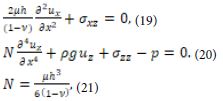
where ν is Poisson’s ratio, N is the flexural rigidity of the elastic plate with thickness h. The displacements  u_x and u_z in the plate are equal to the displacements in the underlying layer at z = 0. The temperature boundary condition is added to the boundary conditions (19) and (20)

The incompressibility condition for a viscous medium, under which equation (14) is valid, is written as

where τ is the characteristic time of the flow under consideration, and K is the bulk modulus. It follows from (23) and (11)

In equations (12) and (13), the inertial terms can be neglected under the condition

from which it follows

Slow flows with a large characteristic time τ are called creeping. Convective flows in the Earth are a typical example of creeping flows. The lithosphere, which exhibits both elastic and viscous properties, is described by the Maxwell viscoelastic rheological model. Elasticity can be neglected for a sufficiently slow flow

where µ is the elastic shear modulus, and η_eff /μ is called the Maxwell time. It follows from condition (27)

To move to dimensionless variables, we introduce the following scales: the length scale is the layer thickness d, the time scale is d²/x , where κ is the thermal diffusivity, the velocity scale is κ/d, the pressure (and stress) scale is kη_A /d², where η_A is the viscosity scale for the Andrade medium. The temperature difference between the hot lower and cold upper surfaces of the layer is taken as the temperature scale. For the Andrade medium η_A = A(d² /x)^2/3, and then with an exponential dependence on time, the dimensionless effective viscosity takes the form

and the Rayleigh number for the Andrade medium is defined as

The lithosphere is characterized by the following values of physical parameters [16]:

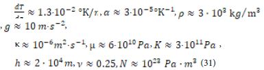
The thickness of the continental lithosphere, which is taken as the length scale, is estimated as d = 2∗ 10⁵ m. Since the Andrade parameter for the lithosphere is estimated as 10¹² Pa∗.s^1/3 m, the Rayleigh number, according to (31), is estimated as Ra ≈ 80.

We will represent the vertical velocity as

where λ is the complex increment, k is the real wave number. We will represent all the physical variables in a similar form. This representation allows us to reduce the system of partial differential equations (12) – (18) to a system of ordinary differential equations, in which all variables characterizing the strain rates, stresses, and pressure depend only on the vertical coordinate z. The characteristic time τ for a flow with a decrement λ can be represented as .

Passing to dimensionless variables and substituting relations (32) into equations (12) – (15), (16) and (18), we obtain relations connecting the amplitudes of pressure, temperature, and components of the deviatoric stress tensor with the amplitude of the vertical velocity

Excluding from the equations the amplitudes of all physical variables, except for the amplitude of the vertical velocity V_z , we arrive at an ordinary differential equation, valid for small values of λ, for which we can neglect elasticity and inertia of the layer (-1 < z <0) simulating the lithosphere,

From (34) it follows that the influence of the temperature gradient can be neglected when

The boundary conditions on the upper deformable surface of layer z = 1 are

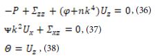
where U_z is the vertical displacement of the upper boundary of the layer, i.e. the deviation of the boundary surface from the plane z = 1. Equations (36) and (37) follow from the condition of equilibrium of the forces acting on a unit area of the disturbed surface of the layer, and equation (38) follows from the condition of vanishing of the temperature disturbance on this surface. Equations (36) and (38) include the displacement of the boundary U_z due to the fact that in the state of equilibrium there is vertical gradients of pressure and temperature in the layer. Condition (38) assumes that the boundary motion is determined by the motion of material points located on this boundary. In equations (36) and (37), dimensionless parameters are introduced:

which characterize the deformable surface. For sufficiently small k, the influence of a thin elastic plate modeling the upper crust is negligible.

Using the parameter φ, the Rayleigh number can be written as  The parameter φ describes the mobility of the boundary and is the ratio of the additional hydrostatic pressure caused by the boundary displacement to the characteristic viscous stress in the layer. The smaller the parameter φ, the more mobile the boundary. For a very large value of φ, the upper surface of the layer behaves like a fixed boundary.

Under each lithospheric plate, there is an isothermal core of large-scale mantle convection, and there is movement with a constant horizontal velocity at the lithosphere-mantle boundary [16]. Therefore, in the coordinate system that moves together with the lithospheric plate, the following conditions must be imposed at the lower boundary of the plate

Thus, the lower boundary of the lithosphere, considered as a boundary layer of large-scale convection, is isothermal (the temperature perturbation is zero at this boundary) and “solid” (zero velocity components at this boundary).

The general solution of the ordinary differential equation (34) is written as

where   q₁ , q₂ , q₃ are the roots of the equation

Investigating surface waves, for which disturbances do not penetrate into the deepest layers of the lithosphere, we consider only sufficiently large values of the wave number (k > 3), for which  e^{q1 z} , e^{q2 z} and e^{q3 z} are close to zero at the lower boundary (z = -1). In this case, to satisfy the boundary conditions at the lower boundary of the lithosphere, it is sufficient to set C₄ = C₅ = C₆ = 0 Substituting (40) into the boundary conditions (36) – (38) on the upper surface, we arrive at a system of three homogeneous equations for three unknowns C_{1 ,} C₂ and C₃. In order for this system to have a solution, it is necessary to equate its determinant to zero

As a result, we obtain the characteristic equation relating the decrement λ to the wave number k. For large wave numbers (k > 5), the imaginary parts of the complex decrements are very small. This means that the temperature gradient present in the lithosphere has a very weak effect and the Rayleigh number in equations (34) and (41) can be neglected. For k = 3, the decrement takes the value . Such a convective wave propagates with the dimensionless velocity . The dimensional velocity of this wave is extremely small: m/year. Values of k < 3 cannot be considered since equation (42) was obtained for surface waves. However, the study of thermoconvective waves [8,9,10,11] allows us to assume that for k < 3 the imaginary part of the decrement and the propagation velocity increase, while the real part of the decrement (attenuation) tends to zero.

The characteristic equation (42) is obtained for sufficiently small values of k and λ, for which the elasticity and inertia of the medium can be neglected. For large values of the wave number k and the decrement λ, the viscosity of the medium and temperature effects can be neglected but the elasticity and inertia of the medium must be taken into account. In this case, it is more convenient, while maintaining the length scale d=2∗ 10⁵ m, to move to the velocity scale  and the time scale Then λ=iw (the decrement becomes purely imaginary), and the characteristic equation takes the form

This equation has solutions w(k) = Vk, where V ≈ 0.95529 is the dimensionless velocity of the surface wave. Its dimensional velocity is slightly lower than the velocity of the bulk transverse wave. Taking into account the effect of gravity (non-zero parameter φ) slightly increases the frequencies ω(k) ≈ 0.95531k. Equation (43) describes the Rayleigh wave in an incompressible medium. Taking into account compressibility, equation (43) becomes

where  This parameter can be considered small, since it has little effect on the result. The frequencies ω found from equation (43) and from equation (44) differ by approximately 3%.

When k and λ are small enough to neglect elasticity and inertia, but not small enough to take into account thermal effects, the complex decrement λ turns out to be a real number (lmλ = 0). In this case, which will be discussed in the next section, there is no wave motion at a fixed k but we can speak of a diffusion – type wave in the presence of a whole spectrum of values of k.

Laplace Transform. Diffusion-type Wave

Solving the problem of excitation of surface waves by the initial disturbance of the Earth’s surface, we will use the Laplace transform with respect to time t and the Fourier transform with respect to the spatial horizontal coordinate x. Representation (32) introduces the Fourier transform but not the Laplace transform, which allows us to find not only solutions of the form exp (λt).

The Laplace transform is a convenient mathematical apparatus for solving differential equations with initial conditions. The Laplace transform f∗(s), denoted by an asterisk, is related to the original f(t) by the equation

The Laplace variable s is a complex number, unlike the Fourier variable k, which is a real wave number.

Using the Laplace transform, we can write the rheological equation (3) as

where G∗_A  is the Laplace analogue of the shear modulus for the Andrade medium, Γ(1/3) ≈ 3 is the gamma function. Equation (7) corresponds to the Laplace image

where G∗ is the Laplace analogue of the shear modulus for an elastic-creeping medium.

As follows from (46), the elasticity of the medium can be neglected if the condition

is satisfied, under which the Laplace analogue of the shear modulus for the Andrade medium G∗_A is significantly less than the elastic shear modulus μ. According to the property of the Laplace transform, it follows from (47)

The compressibility of the medium can be neglected if the Laplace analogue of the shear modulus for the Andrade medium G*_A is significantly less than the elastic bulk modulus K. Since the elastic shear modulus μ is less than the bulk modulus (K ≈ 3μ), condition (48) allows us to neglect not only the elasticity but also the compressibility of the medium. Since μ ≈ 6. 10¹⁰ Pa and A ≈ 10¹² Pa ∗ s^1/3 , it follows from (48) that the lithosphere beneath the elastic upper crust behaves as a creeping Andrade medium, not exhibiting elasticity or compressibility at times exceeding 10⁴ s.

The effect of inertia is negligibly small (inertial forces are small compared to the forces arising during deformations of the Andrade medium), if

The right-hand side of (49) is estimated as 20 s for the lithosphere. Consequently, neglecting elasticity, inertia can be neglected even more so. Isostatic recovery processes with characteristic times not exceeding 10,000 years are slow enough to neglect elasticity, compressibility, and inertia, but are not slow enough to take into account the buoyant Archimedean force, the presence of which is due to the vertical temperature gradient in the lithosphere. The physical variables in equations (12) – (14) depend on the horizontal coordinate x, the vertical coordinate z, and time t. Applying the Fourier transform in the coordinate x and the Laplace transform in time t to these equations and excluding all physical variables except the vertical displacement, we arrive at the relations

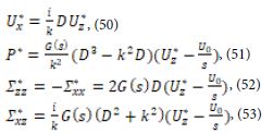
where the differential operator D = d/dz is introduced, and U₀=U₀(x, z) is the initial (t = 0) distribution of vertical displacements. In the equations (50) – (53), the Fourier transforms of the physical variables are denoted by corresponding capital letters, the Laplace images are marked with the asterisk, k is the wave number (the Fourier variable), s is the Laplace variable. Then we obtain the ordinary differential equation for the vertical displacement

The solution of equation (54), which satisfies the boundary condition for z⟶ – ∞, is written as

where C₁ and C₂ are arbitrary integration constants that depend on the Laplace variable, and the wave number k can take negative values. Substitution of the solution (55) into the boundary conditions (19) – (20) allows us to eliminate arbitrary constants and represent the vertical displacement of the upper surface (z = 0) in the form

where G^*_A = As^1/3 is the analog of the shear modulus for the Andrade medium. It should be noted that the substitution of (50) and (53) into the boundary condition (19) leads to the relation C₂ = – C₁ /k, at which horizontal displacements and tangential stresses are absent on the upper surface. Thus, when searching for a solution to equation (54), one can replace the boundary condition (19) with the condition U^*_x= 0 at z = 0 or with the condition Σ^*_xz= 0 at z=0.

In order to find the asymptotic (small times) dependence of the Laplace origin on time, it is sufficient to expand the Laplace image in a series in powers of s in a neighborhood of s = ∞ and invert by Laplace each term of the series [17]. The right-hand side of (24) for s⟶ ∞, is representable in the form of a series

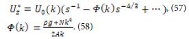
Inverting the terms of the series (57), we obtain the asymptotic dependence of the vertical displacement on time

where the gamma-function at the point 4/3 is estimated as

The asymptotic dependence (59) is valid when

As follows from (60), the asymptotic dependence (59) can be represented in the form

The function Φ(k) has a sharp minimum, which is found from the condition

If we switch to the length scale introduced above d=2∗10⁵ m, this wave number takes the value K_m= 3.6

At large times, the displacements of the surface are described by another asymptotic formula. In the neighborhood of the point s = 0, the right-hand side of equality (56) can be represented as a series  

According to the theorem on the asymptotic behavior of the original [17], the Laplace original at large times can be represented as a series whose terms are obtained as a result of the inverse Laplace transform of each term of the series (64). Keeping only the first term of the expansion, we find

Asymptotic dependence (65) is valid at large times, when

As follows from (65), at large times, harmonics with different wave numbers k decay according to the same law t^-1/3 and the effect of propagation of surface displacements, which occurs at small times, disappears. Since the minimum value of Φ(k) is achieved at k=k_m , inequality (66) is satisfied for any wave numbers if

If the medium underlying the elastic upper crust had the rheology of a Newtonian fluid with viscosity η, the analogue of the shear modulus G^*_A(s) should be replaced by ηs, and equation (56) would be written as

Inversion of the Laplace image (68) yields

where τ is the recovery time, depending on the wave number k. Relation (69) is valid for any times t, in contrast to relation (61), which characterizes the Andrade medium and is valid only for not too large times, limited by condition (60).

Let at the initial instant t = 0 the displacement of the upper surface (z = 0) be given as

The Fourier transform of the function (70) is

and the inverse Fourier transform gives

Inversing the Fourier image (61), we find

In the case when u₀=x is an even function, (73) can be written as

Let the initial displacement have the form of a “step”

If x<-1/2 or x > 1/2 

The Fourier transform for such a “step” has the form

For a sufficiently large width l of the initial perturbation, the values of the function (76) are very small when k > 2π /l, i.e., the wider the perturbation region, the narrower the range of wave numbers k, in which the Fourier image is different from zero. Thus, the integration on the right-hand side of (74) is carried out over the region k<2π/l in the neighborhood of the point k = 0. According to the solution (55), for a fixed wave number k, the isostatic flow causes displacements in the lithosphere, depending on the depth as exp (- kz). Since k < 2π /l, we can say that this flow penetrates into the lithosphere to a depth of the order of l/π. Therefore, the flows arising after the removal of small-scale glaciations or other surface loads (for example, drying salt lakes), for which l does not exceed 200 km, are concentrated in the lithosphere. Caused by large-scale glacial loads (l ≈ 1000 ÷ 3000 km) flows that penetrate into the low mantle and recover isostasy over a period of time of about 10,000 years, are not considered in this paper.

As follows from (76), when the width of the initial perturbation is small (lk << 1), the Fourier transform does not depend on k

The image (77) corresponds to a point initial perturbation

where δ (x) is the delta function

In the case of a point initial perturbation (perturbation of any initial width l can be regarded as a point perturbation when we consider displacements at a sufficient distance from the initial perturbation, that is, for x >> l) , it is possible to obtain an analytic solution of the problem of vertical surface motions. For the point initial perturbation, the dependence of the vertical displacements of the surface on the horizontal coordinate and time is determined by the integral

As follows from (62), the expansion of the function Φ(k) in a power series in the neighborhood of has the form k=k_m

where

The power series (80), which represents the function Φ(k) given by (58), converges when |k-k_m|≤k_m, i.e., the radius of convergence of this series is R=k_m

After changing the variable

the integral (79) takes the form

Equation (83) can be rewritten as

where

The integral on the right-hand side of equality (84) is calculated using the saddle point method used in the theory of functions of a complex variable [18]). The stationary point v_o is found from condition

The function of the complex variable f(v), which is given by (85), has a stationary point

As follows from (87), in a neighborhood of the stationary point v_o, the function f (v) can be represented in the form

Substituting (88) into (84), we obtain

By choosing such a path of integration in the complex plane, which is determined by the saddle-point method, we find the relation

where erf(x) is the error function, and R=k_m is the radius of convergence of the power series (80). At times significantly exceeding 10¹⁰s ≈ 300 years, the condition

It is known that erf(x)=1 for x>>1, and the value erf(x) is close to 1 for x > 1.

Thus, as follows from (79), (89) and (90), the required distribution of the vertical displacements of the surface takes the form

The found solution (92) is valid for sufficiently long times (from several hundreds to several thousand years). The upper bound on time is imposed by condition (60), in which k=k_m.

The graphs in Figure 1 are constructed by the relation (92) and show the dependence of the vertical displacements on the horizontal coordinate at different instants of time.

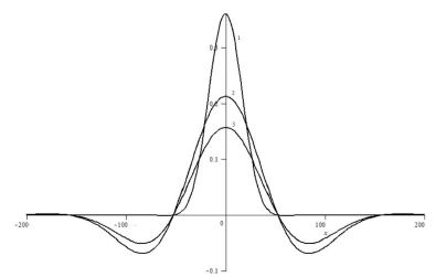
Figure 1: The dependence of the vertical displacements of the Earth’s surface on the horizontal coordinate at different times for the case when the width of the region of the initial displacement l is 10 km. Curve 1 corresponds to 30 years, curve 2 to 300 years, curve 3 to 1000 years.

By differentiating the right-hand side of (92) with respect to t for a fixed value of x, it is not difficult to find the velocity of the vertical motion of the Earth’s surface at points sufficiently far from the region of the initial disturbance of the relief. For example, when u_o= 100 m, l = 10 km, x = 100 km, the velocity  reaches its maximum value (about 1 mm/year) during the time t ≈ 600 years. The generalization of the considered case of the initial point vertical displacement to the 3D problem formulation implies not too much new to understanding of the process under consideration: it is sufficient to replace the coordinate x by the polar coordinate r in Figure 1 (the solution does not depend on the polar angle for the point perturbation of vertical displacement). The initial disturbance of the Earth’s surface leads not only to diffusion-type waves, but also to seismic waves and convective waves. Diffusion-type waves cannot be considered without the initial disturbance, which produces a spectrum of harmonics. Each of these harmonics is not a traveling wave. The wave effect appears only when the entire spectrum is considered.

In the previous section, traveling harmonic waves, both convective and elastic, were considered. The solutions obtained can be represented as

where u_o is the initial vertical displacement of the surface, ω=Imλ, Λ=Reλ, and λ is the found value of the complex decrement (Reλ<0). The use of the Laplace transform allows us to find an arbitrary constant C. To do this, we transform the original equations using the Laplace transform, and substitute the resulting general solution, containing arbitrary constants, into the boundary conditions Laplace transformed. As a result, we find the function F(s, k) and obtain a solution to the problem in the form of a Laplace image

To invert the Laplace image (94), we can use the well-known theorem on the asymptotic behavior of the original [17]. According to this theorem, in order to find an asymptotic solution at large times (t → ∞), it is sufficient to know the Laplace image in the neighborhood of the singular point . In our case, this singular point is a first-order pole, in the neighborhood of which

and the Laplace original has the form

The pole s_o is equal to the complex decrement λ found in the previous section.

Expression (96) is the Fourier image. To pass to the Fourier original, it is necessary to specify the function U_o(k) determined by the initial disturbance. As a result, we can obtain a solution in the form of a running wave packet.

Conclusion

The paper considers disturbances of the Earth’s surface relief caused by an initial small-scale disturbance that disrupts isostasy. The solutions of the equations of continuum mechanics are obtained using the Fourier transform with respect to the spatial horizontal coordinate and the Laplace transform with respect to time [19]. The propagation of vertical displacements along the Earth’s surface from the region of the initial perturbation is carried out by surface waves. At short times, the presence of vertical temperature gradient in the lithosphere can be neglected and a solution in the form of a decaying seismic wave can be obtained. In this case, the creep of the medium, leading to attenuation, is described by the rheological Lomnitz’s law. At very short times, creep can also be neglected, obtaining a solution in the form of an elastic Rayleigh wave. At very long times, the elasticity and inertia of the lithosphere can be neglected but, taking into account the vertical temperature gradient, a solution in the form of a thermoconvective wave can be obtained. At not too large and not too small times, one can neglect not only elasticity and inertia, as in the description of a thermoconvective wave, but also thermal effects, as in the description of Rayleigh waves, obtaining a wave of the diffusion type that occurs in the process of isostasy recovery.

The initial disturbance determines the spectrum of wave numbers k. Elastic Rayleigh waves are characterized by large values of k and propagate very quickly, determining the relief of the Earth’s surface only in the first seconds after the disturbance occurs. Thermoconvective waves are characterized by small values of k (large wavelengths) and propagate very Diffusion-type waves correspond to values of k lying between the wave numbers characteristic of thermoconvective waves and the wave numbers characteristic of Rayleigh waves. The wave character of the solution at short times is due to inertia, and at long times – to the vertical temperature gradient. In the case of Rayleigh and thermoconvective waves, each harmonic moves according to the law , where ω is the frequency and Λ(k) is the decrement. In a diffusion-type wave, each harmonic is motionless, and the harmonic with the wave number (wavelength decays most slowly. Wave motion appears after the inverse Fourier transform due to the dependence of attenuation on k.

Conflict of Interest

The author declares no conflicts of interest in this paper.

References

1. Goetze C (1971) High temperature rheology of Westerly J Geophys Res 76: 1223-1230.
2. Goetze C, Brace WF (1972) Laboratory observations of high-temperature rheology of rocks. Tectonophysics 13: 583-600.
3. Murrell SAF, Chakravarty S (1973) Some new rheological experiments on igneous rock at temperatures up to 1120°C. Geophys J Roy Astron Soc 34: 211-250.
4. Murrell SAF (1976) Rheology of the lithosphere – experimental Tectonophysics 36: 5-24.
5. Berckhemer H, Auer F, Drisler J (1979) High-temperature anelasticity and elasticity of mantle peridotite. Phys Earth planet Inter 20: 48-59.
6. Weertman J (1978) Creep laws for the mantle of the Phil Trans Roy Soc London A 288: 9-26.
7. Karato S (2008) Deformation of Earth An Introduction to the Rheology of Solid Earth. Cambridge university press.
8. Birger BI (1998) Rheology of the Earth and thermoconvective mechanism for sedimentary basins formation. Geophys J Inter 134: 1-12.
9. Birger BI (2000) Excitation of thermoconvective waves in the continental Geophys J Inter 140: 24-36.
10. Birger BI (2012) Transient creep and convective instability of the Geophys J Inter 191: 909 – 922.
11. Birger BI (2013) Temperature-dependent transient creep and dynamics of cratonic Geophys J Inter 195: 695-705.
12. Birger BI (2018) Andrade Creep at the Isostasy Recovering Flows in the Izv Phys Solid Earth 54: 849-858.
13. Birger BI (2007) Attenuation of seismic waves and universal rheological model of the Earth’s Izv Phys Solid Earth 43: 635-641.
14. Birger BI Internal friction in the Earth’ crust and transverse seismic waves. AIMS Geosciences 8: 84 – 97.
15. Cathles LM (1975) The viscosity of the Earth’s mantle. Princeton university press.
16. Turcotte and Schubert G (1982) Geodynamics: Application of Continuum Physics to Geological Problems. New York: John Wiley.
17. von Doetsch G (1974) Introduction to the Theory and Application of the Laplace Transformation.
18. Copson ET (2004) Asymptotic Cambridge University Press.
19. Birger I. (2024) Instability of the Earth’s lithosphere. Cambridge Scholars Publishing.