DOI: 10.31038/GEMS.2023533

Abstract

The excitation of surface and internal water waves by an air pressure wave has been numerically simulated in several model cases, using a nonlinear shallow water model of velocity potential. Water waves were excited when the air pressure wave speed was close to the water wave speed in the surface mode or internal mode. The surface mode waves traveling as free waves after being excited by an air pressure wave  were  also  amplified  by  the shallowing on a sloping seabed. When the air pressure wave with a speed close to that of the internal mode stopped, free surface waves in the internal mode hardly appeared, unlike the free internal waves.

Keywords

Surface wave, Internal wave, Air pressure wave, Proudman resonance, Nonlinear shallow water

Introduction

Internal waves in various waters, such as the East China Sea, e.g., [1,2], and Lake Biwa, e.g., [3,4], may gain large wave heights because the density ratio in water is not as large as that of surface waves. Although various sources of internal waves—tidal currents [5], wind- driven near-inertial waves [6], etc.—have been revealed, the causes of internal waves are unknown in many actual waters.

In the present study, we consider surface/internal wave excitation due to an air pressure wave. Regarding surface waves, air pressure waves of a few hectopascals often generate meteotsunamis around the world, e.g., [7,8,9]. For example, at the west coasts of Kyushu, Japan, meteotsunamis called “Abiki” are observed, e.g., [10,11]. Conversely, internal waves are also generated and amplified by air pressure waves due to meteorological factors including typhoons [12,13]. The excitation mechanism underlying these phenomena is the Proudman resonance [14], which is also known as the cause of other transient waves, e.g., [15,16,17,18,19]. Moreover, the resonance triggered by air pressure waves from a volcanic eruption may generate global tsunamis, e.g., [20,21]. Artificial waves can also be created by the resonance when an airplane moves on a very large floating airport [22].

In this basic research, numerical simulations of surface and internal wave excitations due to an air pressure wave have been generated in several model cases, using a nonlinear shallow water model of velocity potential. Although the wave dispersion and Coriolis force are not considered, the proposed simple model will provide an easy-to-use tool for predicting long-wave excitations from air pressure changes estimated in weather forecasts. We consider the cases in which the air pressure wave speed is close to the surface or internal mode speed.

Method

We consider the irrotational motion of inviscid and incompressible fluids in two layers, as illustrated in Figure 1.

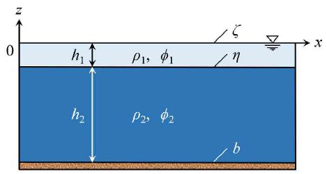
Figure 1: Two-layer water

The still water depths of the upper and lower layers are h₁(x) and h₂(x), respectively, and h(x) = h₁(x) + h₂(x). We assume that the densities of the upper and lower layers, ρ₁ and ρ₂, respectively, are uniform and constant, and that the fluids do not mix even in motion. The water surface displacement, interface displacement, and seabed position are denoted by ζ(x, t), η(x, t), and b(x), respectively. Friction is ignored everywhere for simplicity. The velocity potentials of the upper and lower layers are ϕ₁(x, t) and ϕ₂(x, t), respectively.

The nonlinear shallow water equations of velocity potential considering the pressure on the water surface, p₀(x, t), are

Upper Layer

∂η/∂t = ∂ζ/∂t + ∇[(ζ – η) ∇ϕ₁],      (1)

∂ϕ₁/∂t = – [gζ + p₀ /ρ₁ + (∇ϕ₁)²/2],      (2)

Lower Layer

∂η/∂t = –∇ [(η – b) ∇ϕ₂],       (3)

∂ϕ₂ /∂t = – [gη + (p₁ + P₂ )/ρ₂  + (∇ϕ₂ )²/2],      (4)

where ∇ = (∂/∂x, ∂/∂y) is a horizontal partial differential operator. The gravitational acceleration g is 9.8 m/s², p₁(x, t) is the pressure at the interface, and P₂ = (ρ₂ – ρ₁)gh₁. Equations (1)–(4) can be derived by reducing the nonlinear equations based on the variational principle [23].

Substituting Equation (3) into Equation (1), we obtain

∂ζ/∂t = – {∇ [(ζ – η) ∇ϕ₁] + ∇ [(η – b) ∇ϕ₂]}.       (5)

In the upper layer, reversing the direction of the integration with respect to z gives the following auxiliary equation as

∂ϕ₁/∂t + gη + p₁/ρ₁  + (∇ϕ₁)²/2 = 0,      (6)

which corresponds to the Bernoulli equation on z = η.

By substituting Equation (2) into Equation (6), we obtain

p₁  = p₀  + ρ₁ g(ζ – η),       (7)

which expresses the hydrostatic pressure distribution. By substituting Equation (7) into Equation (4), we obtain

∂ϕ₂/∂t = – [gη + p₀/ρ₂ + r^-1g(ζ – η) + (1 – r^-1)gh₁ + (∇ϕ₂)²/2], (8)

where r = ρ₂/ρ₁ > 1.

By eliminating p1 from Equations (4) and (6), we obtain

∂ϕ₁/∂t – r∂ϕ₂ /∂t = (r – 1)g(η + h₁) – [(∇ϕ₁ )² – r(∇ϕ₂)²]/2.                   (9)

We explicitly solve the above equations using a finite difference method with the central difference in space and the forward difference in time. When the pressure at the water surface, p₀, is known and the water surface displacement ζ is unknown, the procedure shown in

Figure 2 is repeated, starting from the initial still water state, to obtain new time-step values one after another.

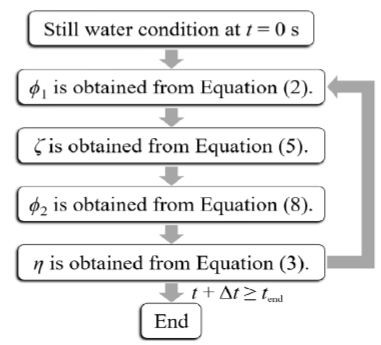
Figure 2: Procedure for obtaining the surface displacement ζ，interface displacement η, and velocity potentials in the upper and lower layers, ϕ₁ and ϕ₂, respectively, when the pressure at the water surface, p₀, is given.

Conversely, when the pressure at the water surface, p₀, is unknown and the water surface displacement ζ is known, we adopt the procedure shown in Figure 3, which was not used in the present calculations.

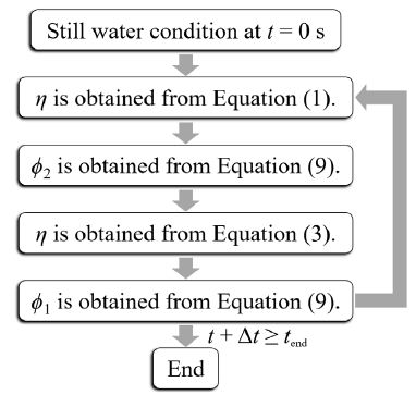
Figure 3: Procedure for obtaining the interface displacement η and velocity potentials  in the upper and lower layers, ϕ₁  and ϕ₂, respectively, when the surface displacement ζ  is given.

Conditions

Focusing on one-dimensional wave propagation in the x-axis direction, we assumed that a steady air pressure wave W, as sketched in Figure 4, traveled in the positive direction of the x-axis with a constant speed v_P. The waveform of the air pressure wave was an isosceles triangle, where the length of its base, i.e., the wavelength λ, was 10 km or 20 km. The maximum and minimum pressures p_m of positive and negative air pressure waves, respectively, were 2hPa and −2 hPa, respectively, referring the values in the meteotsunami and eruption cases [11,21]. The position of the air pressure wave center at the initial time, i.e., t = 0 s, was x₀ = 50 km.

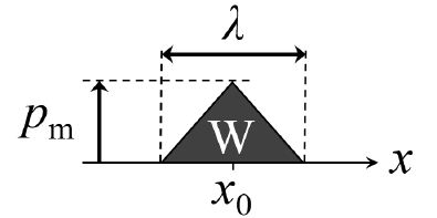
Figure 4: Waveform of the steady air pressure wave W at the initial time, i.e., t = 0 s. The air pressure wave traveled in the positive direction of the x-axis with constant speed v_p.

The densities of the upper and lower layers were ρ₁ = 1000 kg/m³ and ρ₂ = 1025 kg/m³, respectively. Both the initial velocity potentials ϕ₁(x, 0 s) and ϕ₂(x, 0 s) were 0 m²/s. The grid width Δx was 250 m and the time step interval Δt was 1 s.

Excitation of the Surface Mode

In Figure 4, the wavelength λ and the maximum pressure p_m of the air pressure wave were 10 km and 2 h Pa, respectively. In the initial still water state, the total water depth h was 5000 m and the upper layer depth h₁ was 1000 m, in Figure 1. For linear shallow water waves, the phase velocity of the surface mode, C_s, is √(gh) ≃ 220 m/s. When the traveling velocity of the air pressure wave, v_p, is 207 m/s, which is close to C_s , the time variations of the air pressure distribution and both the surface and interface profiles are depicted in Figure 5, in which the results for 100 s ≤ t ≤ 1000 s are displayed every 100 s.

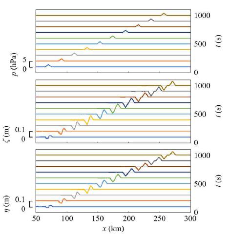
Figure 5: Time variations of the air pressure distribution, surface profile, and interface profile every 100 s. The still water depth h was 5000 m and the still water depth ratio h₁/h was 0.2. The wavelength λ, maximum pressure p_m, and speed v_p of the air pressure  wave were 10 km, 2 hPa, and 207 m/s, respectively.

Figure 5 indicates that the crests and troughs in the surface mode were excited by the Proudman resonance not only at the surface but also at the interface, because the positions of the surface and interface were relatively close. When t = 100 s, the water wave crests have been generated at the air pressure rise, whereas the water wave troughs at the air pressure fall. The length of the water wave crests and troughs was approximately half the wavelength of the air pressure wave. Thereafter, the water wave crests gradually led away from the air pressure wave because the surface mode speed was greater than the air pressure wave speed. When t = 1000 s, the water wave crests were propagating as free waves, whereas the water wave troughs have been constrained by the air pressure wave, and the wavelength of each crest and trough was approximately the same as that of the air pressure wave.

When the seabed is partially sloping, Figure 6 depicts the numerical results for the same conditions as in the case above, except for the topography, where the seabed position b is described as

b = −5000 m for 0 ≤ x < 150 km,

b = −3500 m − 1500 m × cos π (x/150 km – 1) for 150 km ≤ x ≤ 300 km. (10)

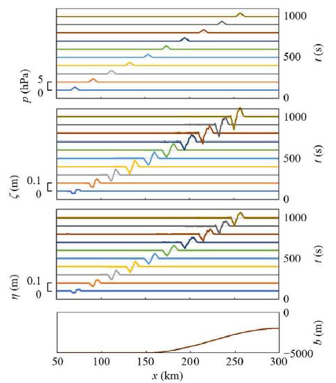
Figure 6: Time variations of the air pressure distribution, surface profile, and interface profile every 100 s. The seabed profile is also depicted, where the seabed position b is described by Equation (10). The initial water depth in the upper layer, h₁ was 1000 m. The wavelength λ, maximum pressure p_m, and speed v_p of the air pressure wave were 10 km, 2 hPa, and 207 m/s, respectively.

As indicated in Figure 6, the second peaks of water wave crests were generated when the air pressure wave speed approached the surface mode speed on the slope. Moreover, both the water wave crests and troughs were amplified by shallowing on the slope after they moved away from the air pressure wave. It should be noted that the shallowing effect requires water waves that are traveling as free waves apart from the air pressure waves that excited the water waves. When an eruption creates air pressure waves with different speeds, as in the case of the 2022 Hunga Tonga–Hunga Ha`apai volcanic eruption,  the air pressure waves excite tsunamis at water depths corresponding to the air pressure wave speeds [24], and each tsunami traveling apart from the air pressure wave that excited it can be amplified by shallowing on a ridge, shelf slope, continental shelf, etc. Tsunamis traveling as free waves after being excited by air pressure waves may also be amplified by being passed by subsequent air pressure waves over topography [21], as indicated in the water wave crests at t = 1000 s in Figure 6. Moreover, bay oscillations, currents, and horizontally two-dimensional changes in topography may amplify tsunamis, similar to submarine earthquake tsunamis.

Excitation of the Internal Mode

The wavelength λ and the maximum pressure p_m of the air pressure wave were 10 km and 2 hPa, respectively, in Figure 4. The still water depth h was uniformly 5000 m, and the still water depth ratio h₁/h was 0.2, in Figure 1. The internal mode speed for linear shallow water waves without surface waves is

so C_i ≃ 14 m/s in the present case. We assumed that while 0 s ≤ t < 1000 s, the air pressure wave speed v_p was 14 m/s, which was almost equal to C_i, whereafter the air pressure wave stopped at t = 1000 s, and the air pressure distribution was stagnated for t ≥ 1000 s. The time variations of the air pressure distribution and both the surface and interface profiles are depicted in Figure 7, in which the results for 200 s ≤ t ≤ 2000 s are displayed every 200 s.

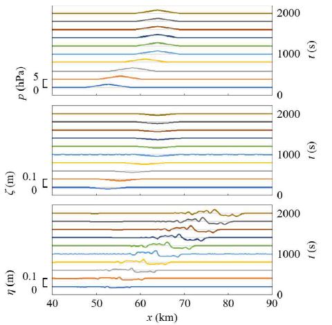
Figure 7: Time variations of the air pressure distribution, surface profile, and interface profile every 200 s. The still water depth h was 5000 m and the still water depth ratio h₁/h was 0.2. The wavelength λ, maximum pressure p_m, and speed v_p of the air pressure wave were 10 km, 2 hPa, and 14 m/s, respectively.

Based on Figure 7, the internal waves in the internal mode were excited by the Proudman resonance, and especially the crest was amplified remarkably. Conversely, free surface waves in the internal mode hardly appeared because the surface wave crest was constrained by the stagnant air pressure distribution.

When the wavelength λ and the minimum pressure p_m of the air pressure wave are 20 km and −2 hPa, respectively, Figure 8 presents the numerical results for the same other conditions as in the above case.

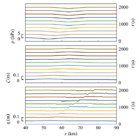
Figure 8: Time variations of the air pressure distribution, surface profile, and interface profile every 200 s. The still water depth h was 5000 m and the still water depth ratio h₁/h was 0.2. The wavelength λ, minimum pressure p_m, and speed v_p of the air pressure wave were 20 km, −2 hPa, and 14 m/s, respectively.

In Figure 8, the waveform of the generated internal waves propagating as free waves is different from the vertically inverted waveform of the above-mentioned internal waves due to the air pressure wave of positive pressure, disregarding the difference in wavelength. Therefore, future work is required to investigate the stability of the upward and downward convex internal waves due to an air pressure wave, considering higher-order terms of the velocity potential.

Conclusion

The excitation of surface and internal water waves by an air pressure wave was numerically simulated using the nonlinear shallow water model of velocity potential. The water waves were excited when the air pressure wave speed was close to the water wave speed in each mode. The surface mode waves traveling as free waves after being excited by an air pressure wave were also amplified by the shallowing on the sloping seabed. When the air pressure wave, the speed of which was close to the internal mode speed, stopped, free surface waves in the internal mode hardly appeared, unlike the free internal waves.

In the present model, wave dispersion is ignored, so in the future, the excitation of relatively shorter water waves by air pressure waves should be investigated using a numerical model with higher-order terms of velocity potential.

Conflicts of Interest

The author declares no conflict of interest.

References

1. Hsu MK, Liu AK, Liu C (2000) A study of internal waves in the China Seas and Yellow Sea using Continental Shelf Research 20 : 389-410.
2. Nam S, Kim Dj, Lee SW, Kim BG, Kang Km, Cho YK (2018) Nonlinear internal wave spirals in the northern East China Scientific Reports 8.
3. Kanari S (1973) Internal waves in Lake Biwa (H)—numerical experiments with a two layer model. Bulletin of the Disaster Prevention Research Institute 22 : 70-96.
4. Jiao C, Kumagai M, Okubo K (1993) Solitary internal waves in Lake Bulletin of the Disaster Prevention Research Institute 43 : 61-72.
5. Hibiya T (1988) The generation of internal waves by tidal flow over Stellwagen Journal of Geophysical Research 93 : 533-542.
6. Le Boyer A, Alford MH (2021) Variability and sources of the internal wave continuum examined from global moored velocity Journal of Physical Oceanography 51: 2807-2823.
7. Vilibić I, Monserrat S, Rabinovich A, Mihanović H (2008) Numerical modelling of the destructive meteotsunami of 15 June, 2006 on the coast of the Balearic Islands. Pure and Applied Geophysics, 165 : 2169-2195.
8. Bailey K, DiVeglio C, Welty, A (2014) An examination of the June 2013 East Coast meteotsunami captured by NOAA observing systems. NOAA Technical Report, NOS CO-OPS 079.
9. Niu X, Zhou H (2015) Wave pattern induced by a moving atmospheric pressure disturbance. Applied Ocean Research 52 : 37-42.
10. Hibiya T, Kajiura, K (1982) Origin of the Abiki phenomenon (a kind of seiche) in Nagasaki Journal of the Oceanographical Society of Japan 38 : 172-182.
11. Kakinuma T (2019) Long-wave generation due to atmospheric-pressure variation and harbor oscillation in harbors of various shapes and countermeasures against meteotsunamis. In Natural Hazards—Risk, Exposure, Response, and Resilience; Tiefenbacher JP, Ed : IntechOpen: London, Pg : 81-109.
12. Geisler JE (1970) Linear theory of the response of a two layer ocean to a moving hurricane. Geophysical and Astrophysical Fluid Dynamics 1 : 249-272.
13. Dotsenko SF (1991) Generation of long internal waves in the ocean by a moving pressure zone. Soviet Journal of Physical Oceanography 2 : 163-170.
14. Proudman J (1929) The effects on the sea of changes in atmospheric Geophysical Journal International 2 : 197-209.
15. Whitham GB (1974) Linear and Nonlinear Waves, John Wiley & Sons, Inc.: New York, NY, Pg : 511-532.
16. Lee S, Yates G, Wu T (1989) Experiments and analyses of upstream-advancing solitary waves generated by moving disturbances. Journal of Fluid Mechanics 199 : 569-593.
17. Kakinuma T; Akiyama M (2007) Numerical analysis of tsunami generation due to seabed deformation. In Coastal Engineering 2006; Smith JM, Ed : World Scientific Publishing , Pte. Ltd.: Singapore. Pg : 1490-1502.
18. Dalphin J, Barros R (2018) Optimal shape of an underwater moving bottom generating surface waves ruled by a forced Korteweg-de Vries Journal of Optimization Theory and Applications 180 : 574-607.
19. Michele S, Renzi E, Borthwick A, Whittaker C, Raby A (2022) Weakly nonlinear theory for dispersive waves generated by moving seabed deformation. Journal of Fluid Mechanics 937.
    
20. Garrett CJR (1970) A theory of the Krakatoa tide gauge disturbances. Tellus 22 : 43- 52.
21. Kakinuma T (2022) Tsunamis generated and amplified by atmospheric pressure waves due to an eruption over seabed Geosciences 12.
22. Kakinuma T, Hisada M (2023) A numerical study on the response of a very large floating airport to airplane Eng 4 : 1236-1264.
23. Kakinuma T (2003) A nonlinear numerical model for surface and internal waves shoaling on a permeable beach. In Coastal Engineering VI; Brebbia CA, Lopez- Aguayo F, Almorza D, Eds : Wessex Tech. Press, Pg : 227-236.
24. Yamashita K, Kakinuma T (2022) Interpretation of global tsunami height distribution due to the 2022 Hunga Tonga-Hunga Ha’apai volcanic Preprint available at Research Square.