Abstract
In this paper, the spectral characteristics of seismic data obtained at various seismic stations in Antarctica are studied using the spectral histogram method developed by the authors and the study of regional structures. This takes into account the fundamental features of the geological, geophysical and astrophysical picture of the entire continent; significant component of fragile crustal structures. The possibility of the existence in the polar region of the ancient structures of the plume during its formation experienced the impact of centrifugal forces from the rotation of the Earth and the inhibition of the top of the plume in the low-temperature near-surface layer. One of the most significant attractions of the region is the existence of a large-sized ozone “hole”. All the above features have found their reflection in the seismic fields of Antarctica.
Keywords
Antarctica, seismic fields, plume tectonics, ozone holes, modulated solar wind, solar oscillations
Introduction
Probable plume tectonics It is likely that the Antarctic bears the signs of a super plume (Fig. 1). A similar example of a modern “hot spot” is about. Iceland. The thickness of the ocean-type crust under this island reaches 40 km. (usually the thickness is 7 km). Paleo – Iceland’s counterparts – a giant Antarctic uplift, etc. Until now, volcanic activity has been observed in Antarctica (Figure 1).
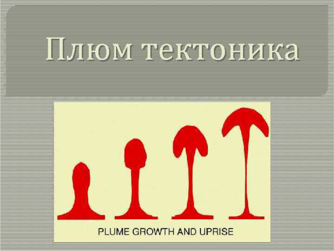
Figure 1. There is an example of the plume development. At the final stage, the tip of the Antarctic plume, due to the anomalously cooled surface rocks of the crust, will assume a more subtle and probably not continuous form.
The modern map of Antarctica quite well shows similarities with the elements of the super – plume (Fig. 2.) (Figure. 2a,b).
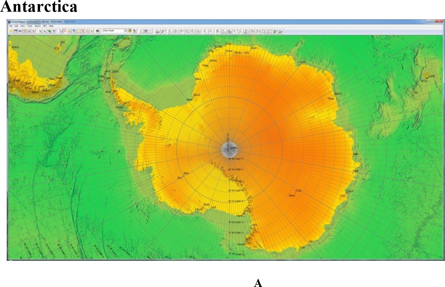
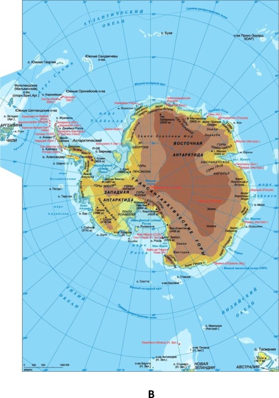
Figure 2. A, B. This is modern map of Antarctica. With the exception of the peninsula, the coasts are rounded, forming a super plume.
Given the thickness of the ice cover (up to 9 km), and the structure of the crustal rocks, as well as thermal and coastal processes, we should expect the existence of various seismic fields. In addition, there are many caves in the coastal zone, possibly remnants from the periphery of the plume. During the Second World War, a submarine base of Germany existed in the caves off the coast. There is the existence of the ozone hole over the continent. Large-scale, ozone-free atmospheric space above the continent (Figure 3) makes radical additions to the description of Antarctic seismicity. There are such effects that are impossible for terrestrial seismicity. The absence of ozone protection makes available the effect on the surface of many solar processes: radiation (from ultraviolet radiation to x-rays and gamma radiation), solar cosmic rays and flares, muons, modulated solar wind and interplanetary shock waves (MUV). A similar picture is observed for lunar seismicity. Many of the effects are almost constantly modulated, for example, by solar oscillations which make it possible to observe waves at solar frequencies in the spectrum of the seismic field (Table 1).
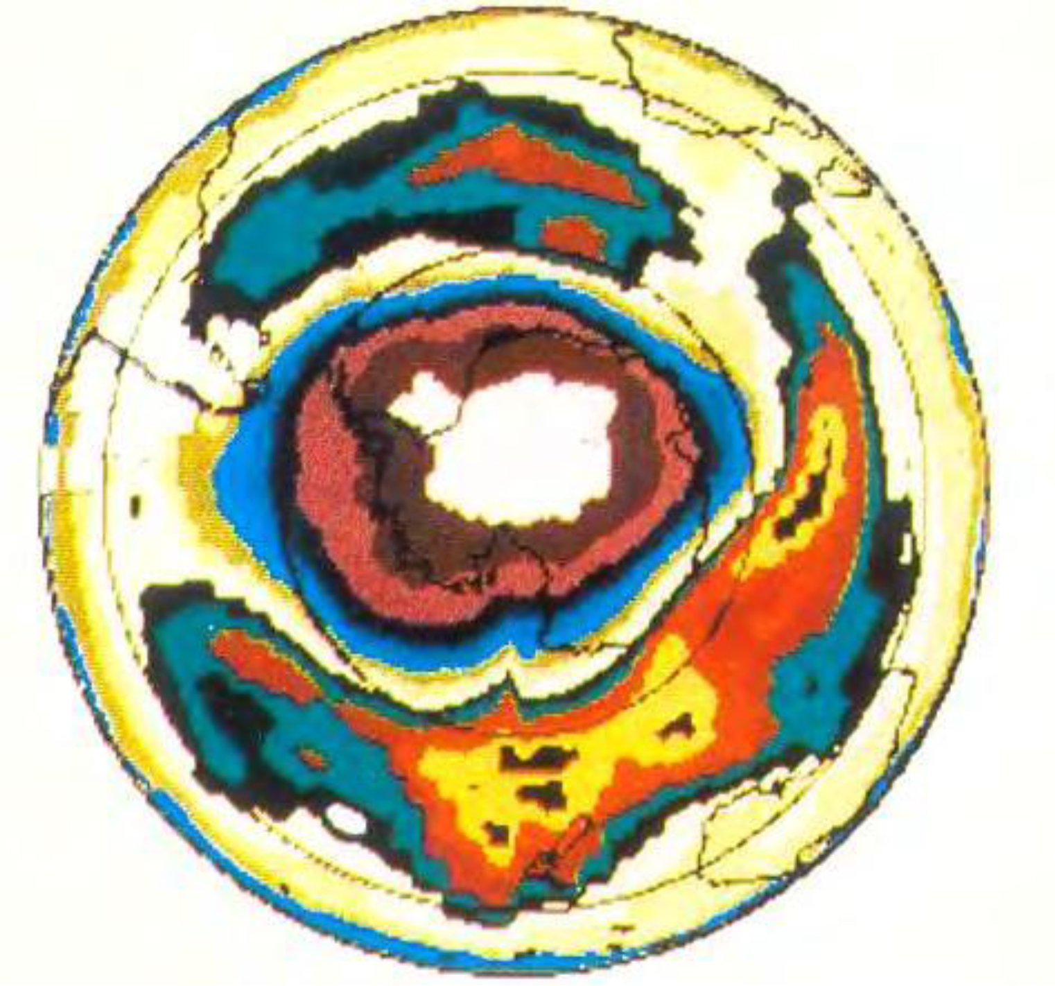
Figure 3. Map of the ozone hole over Antarctica.
Table 1. Periods of oscillations of the standard model of the Sun with the relative content of heavy elements Z = 0.02 according to calculations by Iben n Makhefi
|
Mode |
Period (min) |
Mode |
Period (min) |
|||||||
|
l=0 |
l=1 |
l=2 |
l=3 |
l=4 |
l=1 |
l=2 |
l=3 |
l=4 |
||
|
p1 |
62,29 |
57,25 |
42,50 |
39,53 |
37,58 |
f |
|
45,90 |
40,97 |
38.82 |
|
p2 |
40,94 |
36,98 |
32,19 |
29,42 |
27,62 |
g1 |
61,58 |
55,05 |
47.94 |
44,15 |
|
P3 |
30,93 |
27,88 |
25,09 |
23,21 |
21,92 |
g2 |
84,4 |
63.03 |
54.88 |
49,59 |
|
p4 |
24,49 |
22,30 |
20,52 |
19,26 |
18,31 |
g 3 |
105,3 |
72,58 |
61.88 |
57,73 |
|
p5 |
20,19 |
18,08 |
17,39 |
16,44 |
15,72 |
g 4 |
127,3 |
83,49 |
67,78 |
61,11 |
|
p6 |
17,17 |
16,04 |
15,10 |
14,38 |
13,81 |
g 5 |
148.2 |
95.38 |
74,9 |
64,89 |
|
p7 |
14,93 |
14,08 |
13,35 |
12,77 |
12,32 |
g 6 |
171,1 |
107,7 |
88,1 |
70,30 |
|
p8 |
13,21 |
12.55 |
11,97 |
11,51 |
11,14 |
g 7 |
|
120,2 |
91,8 |
76.83 |
|
p9 |
11,85 |
11,34 |
10,87 |
10,49 |
10,18 |
g 8 |
|
132.9 |
100,7 |
83.62 |
|
p10 |
10,78 |
10.35 |
9,97 |
9,85 |
9,39 |
g 9 |
|
145.9 |
109,7 |
90,56 |
|
p11 |
9,90 |
9,54 |
9.21 |
8.94 |
8,71 |
g 10 |
|
158,9 |
118,9 |
97,62 |
|
p12 |
9.15 |
8,84 |
8,56 |
8,32 |
8,11 |
g 11 |
|
172.1 |
128,1 |
104,5 |
|
p23 |
8,50 |
8,25 |
7,99 |
7.78 |
7.60 |
g 12 |
|
|
137,8 |
111,7 |
|
p14 |
7.94 |
7,71 |
7,49 |
7,31 |
7,15 |
g 23 |
|
|
147,0 |
118,9 |
|
p15 |
7.45 |
7,25 |
7,06 |
6,89 |
6,75 |
g 14 |
|
|
156.5 |
126,5 |
|
p16 |
7.02 |
6,84 |
6,67 |
6,52 |
6,39 |
g 15 |
|
|
166,7 |
133,3 |
|
p17 |
6.64 |
6,47 |
6,32 |
6,18 |
6,06 |
g 16 |
|
|
175,9 |
141,5 |
|
p18 |
6.39 |
6.14 |
6,00 |
5,87 |
5,77 |
g 17 |
|
|
|
148,6 |
|
p19 |
5.98 |
5,84 |
5,71 |
5,60 |
5,50 |
g 18 |
|
|
|
156,4 |
|
p20 |
5.69 |
5,58 |
5,45 |
5.34 |
5.25 |
g 19 |
|
|
|
164,0 |
|
|
|
|
|
|
|
g 20 |
|
|
|
171,1 |
In Table 1: p, g, f-modes of the natural oscillations of the Sun; L-form of natural oscillations.
Moreover, the excitation of these waves is not due to the indirect interaction of terrestrial radioactive geological structures with solar neutrinos, but directly. This means that instrumental and methodological development of seismic expeditions to the Moon, Mars and other space bodies devoid of ozone protection should be carried out on Antarctica, as the closest to the external conditions of the landfill (Figure 3).
The ozone hole over the Antarctic and its adjacent territories is quite dynamic: it grew for the first time in recent years, covering an area of 28 million square kilometers (press service of the NASA Goddard Space Flight Center). Previously, the ozone layer was considered to be a natural shield that protects the surface of the Earth from hard ultraviolet radiation, which is dangerous to living organisms. Now it is a parameter of the atmosphere, which allows studying the Sun, solar-terrestrial relations and some astrophysical problems. A sharp drop in the concentration of stratospheric ozone during the winter season was first detected over the Antarctica in the 1980s. Every winter, the ozone hole over Antarctica grows, reaching a maximum area in September, and shrinking in summer. Large sizes fully correspond to how ozone behaves in relatively cold weather in the upper atmosphere of the Earth (Paul Newman, Paul Newman, USA). Due to the slow reduction, the thickness of the ozone layer in some deep regions of the Antarctic has fallen to absolute zero for the first time in many years. This means that the Suns freely “bombard” the polar ice that is under similar areas, for example, the Amundsen – Scott station at the South Pole. The level of ozone began to fall sharply in September, with the result that its concentration decreased by 95% by the first of October. This year, the fall continued for two “extra weeks”, which led to a 100% decrease in the level of ozone by October 15”says another climatologist, Brian Johnson, USA. However, the smaller ozone hole in 2017 is the result of natural variability and is not necessarily a signal of rapid “healing”. Scientists use the word “hole” as a metaphor for an area in which the ozone concentration falls below the historical threshold of 220 Dobson units. A sharp drop in the concentration of stratospheric ozone during the winter season was first discovered over Antarctica in the 1980s. The reason for this was the release of a large number of Freon’s into the atmosphere of the Earth, whose molecules destroy ozone in the upper layers of the atmosphere at low air temperatures. Every winter, the ozone hole over Antarctica grows, reaching a maximum area in September, and shrinking in summer. January 29, 2016, 14:31 – January 27, a huge ozone hole covered northern Eurasia from the Atlantic to the Pacific Ocean. Most of it fell on the territory of Russia. The anomaly center is located in the north of Western Siberia, however, the effect of ozone holes is not yet known to seismologists. Observations in 2017 showed that the hole in the ozone layer of the Earth, which forms over Antarctica at the end of the southern winter, has become the smallest since 1988. According to NASA satellites, the ozone hole reached its one-year maximum of September 11, spreading to 7.6 million square miles (19.6 sq. km), which is 2.5 times the area of the United States. Ground-based measurements and measurements from balloons, carried out by the National Oceanic and Atmospheric Administration, confirmed satellite data. Since 1991, the average maximum area of ozone holes has been approximately 26 million square kilometers (Fig. 4.) (Figure 4).
In view of the above, a start was made to study the seismic fields of Antarctica (Figure 5).
As follows from Figure 5, considerable seismic material has been collected and processed, primarily relating to the coastal zone and partly of the shelf The IRIS Data Management Center (IRISDMC): http://service.iris.edu/fdsnws/dataselect/1/. The study of data was started with spectral analysis (see Fig. 6) (Figure 6).
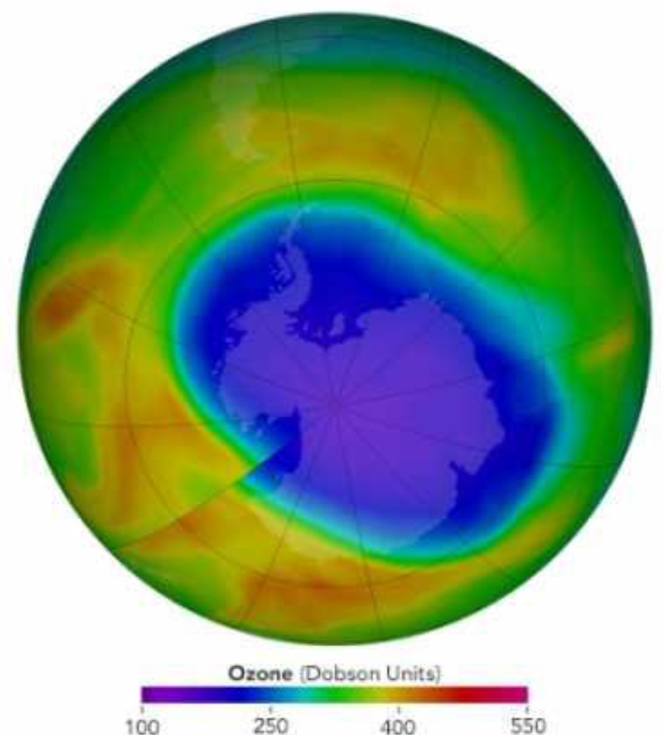
Figure 4. Concentration of ozone over Antarctica. October, 2017. © NASA
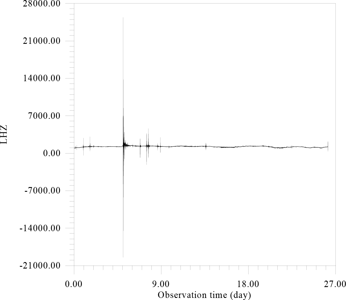
Figure 5. Seismic recording of LHZ-component 60 channel Streckeisen STS-2.5 sensor IU network of QSPA station (89.9289°S, 144.4382°E). The record contains 2265013 seconds. For convenience, the graphical representation is averaged over 120 points in 1 minute increments.
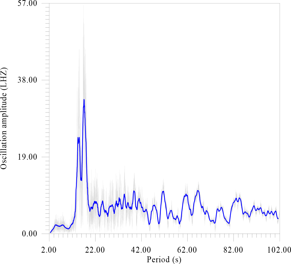
Figure 6. There is amplitude spectrum of seismic data in the range from 2 to 102 sec. in increments of 0.01 seconds. with averaging values of 1 sec.
According to fig.6 the spectrum of seismicity has two peaks dominant in amplitude, for 18 and 20 sec., which, probably, given the proximity of the ocean, should be referred to as “storm” and note also the existence of resonant structures at the Antarctic ice sheet (Figure 7).
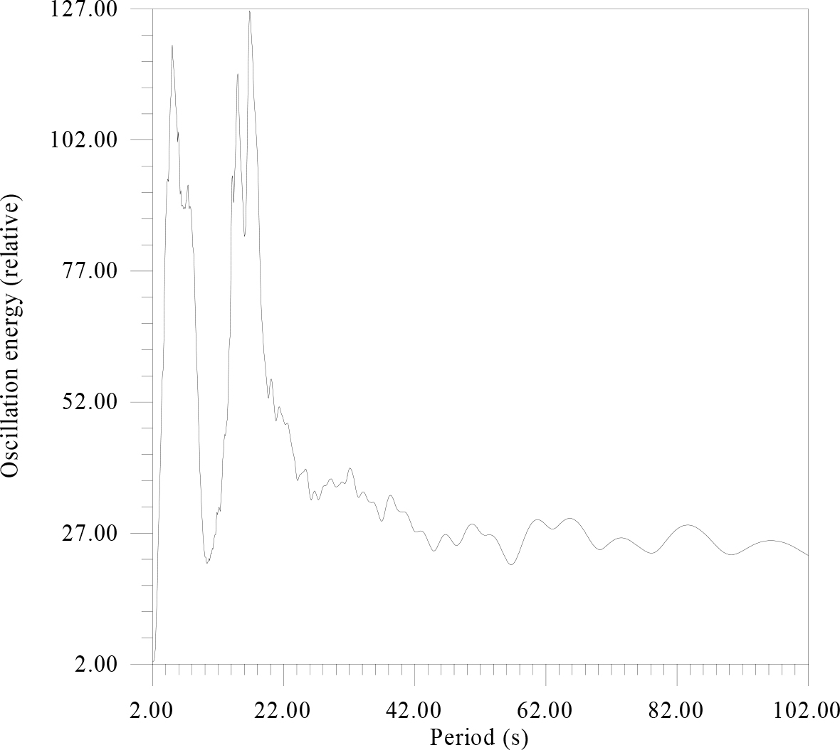
Figure 7. There is the energy spectrum of data Figure 6.
The energy spectrum revealed a more subtle structure of the peaks, at 4 and 18 sec. These peaks are not uncommon when considering seismic fields of complexly constructed and non-linear structures. For greater clarity, the same seismic material was processed by a more complex, but informative method (Fig.8 A, B) (Figure 8 a,b).
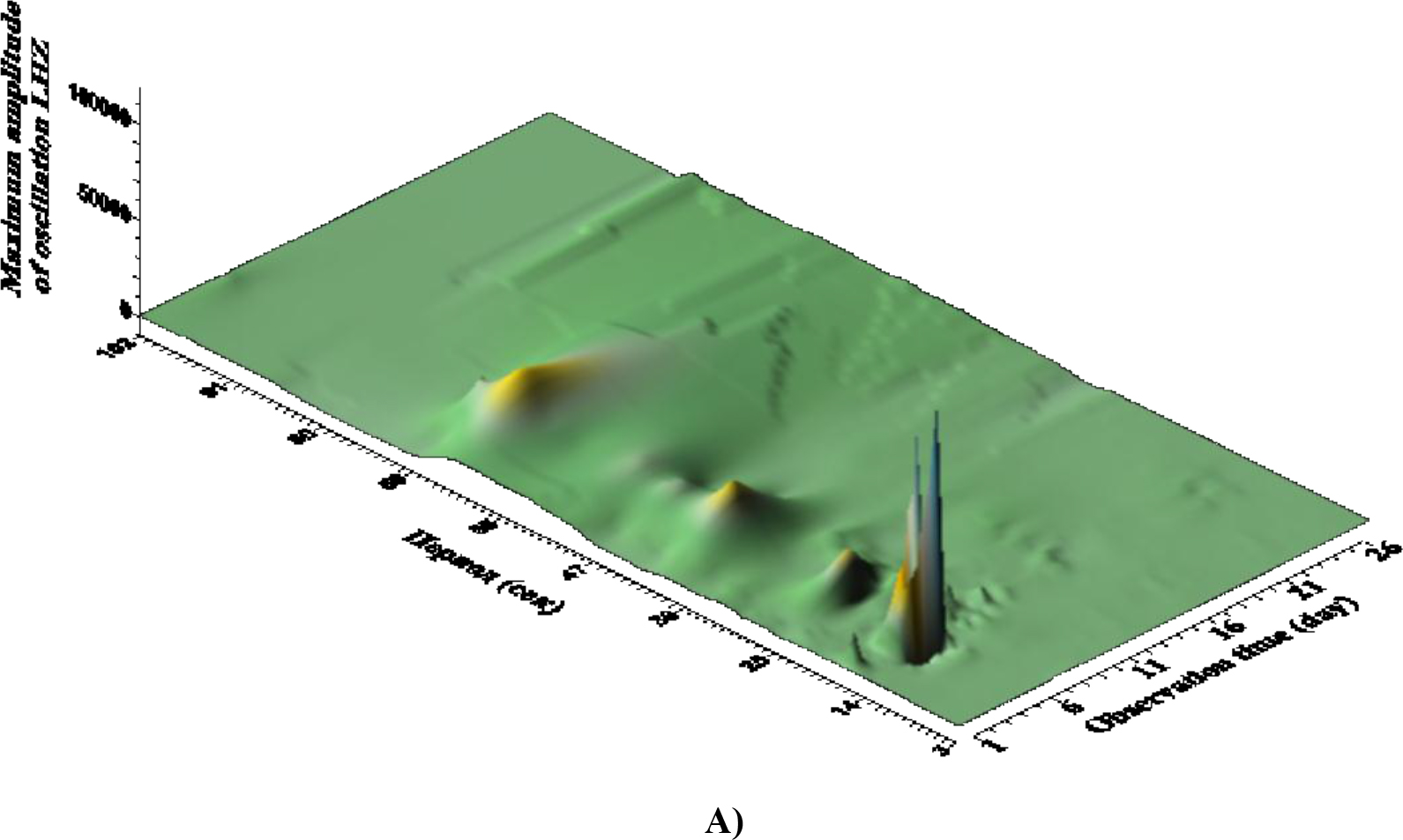
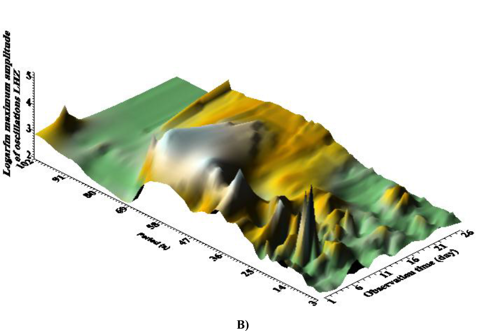
Figure 8. A, B. These are dependence of the maximum amplitude of seismic vibrations A) and its logarithm B), from the observation time and the corresponding period. The interval of the period change is from 2 to 102 sec with a step of 0.1 sec. The time step is 2 minutes (120 seconds). The window is 628 seconds.
According to Fig. 8 (A) for several days, resonant peaks of good quality on micro seismic periods of 14–20 sec can be observed in the wave field; their double period manifests itself in the form of ill-galling small amplitude manifestations. According to Fig. 8 (B) in Antarctica in the general seismic wave field it is possible to distinguish three groups of waves with ranges of periods: relatively high-frequency (periods 3–25 seconds), the longest and with maximum amplitude (periods 49–60 seconds) and short duration of existence as a single peak on period ~ 100 sec. Probably, the longest are associated with existing in the coastal zone and on the shelf of the network of caves and channels (Figure 9).
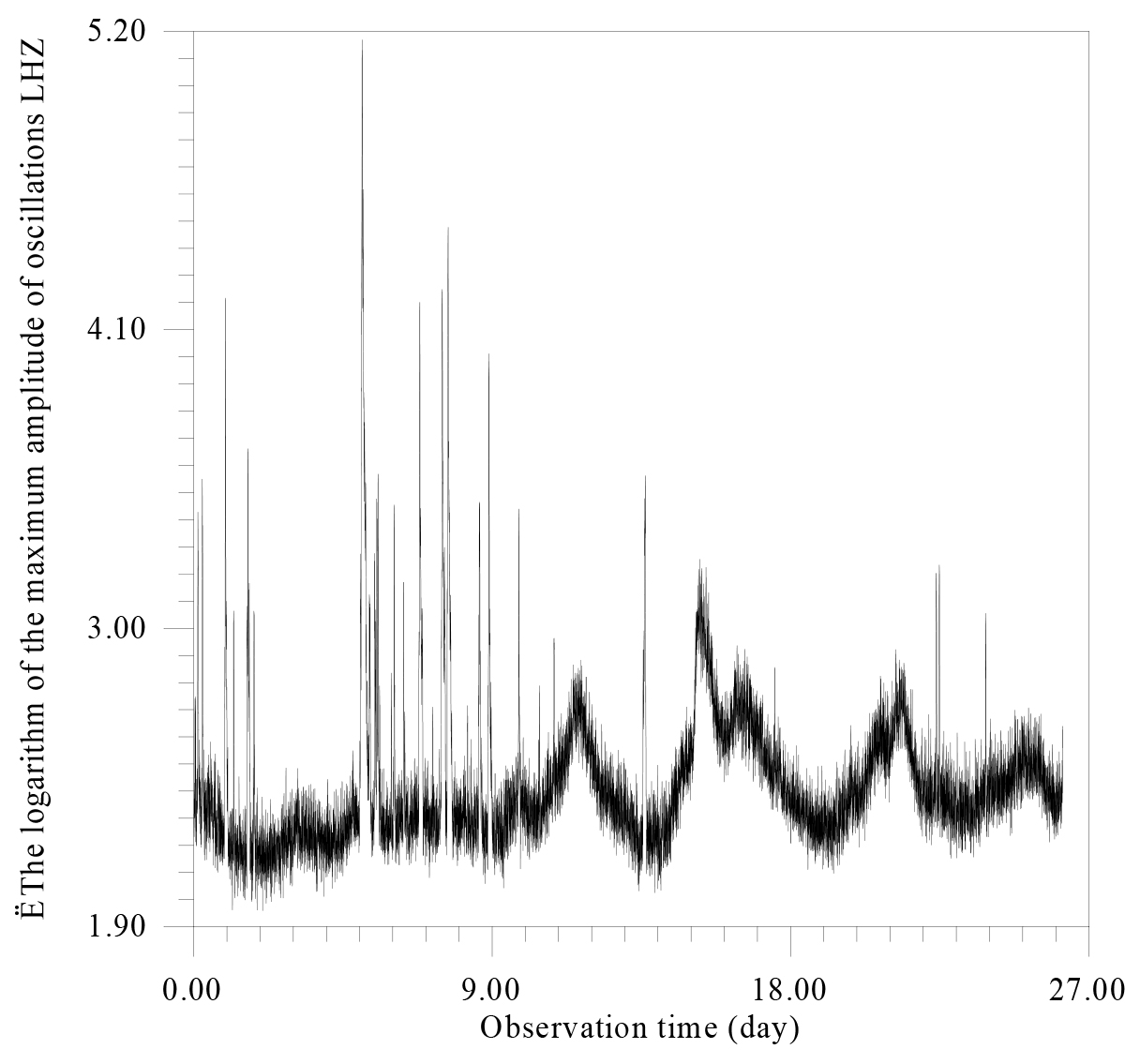
Figure 9. There is the dependence of the logarithm of the maximum amplitude of oscillations on the observation time.
According to Fig. 9, there are two independent types of noise – one high-frequency, constantly existing with an unstable modulation frequency (~ 4–5 days) and the second in the form of very short irregular high-amplitude emissions (Figure 10,11).
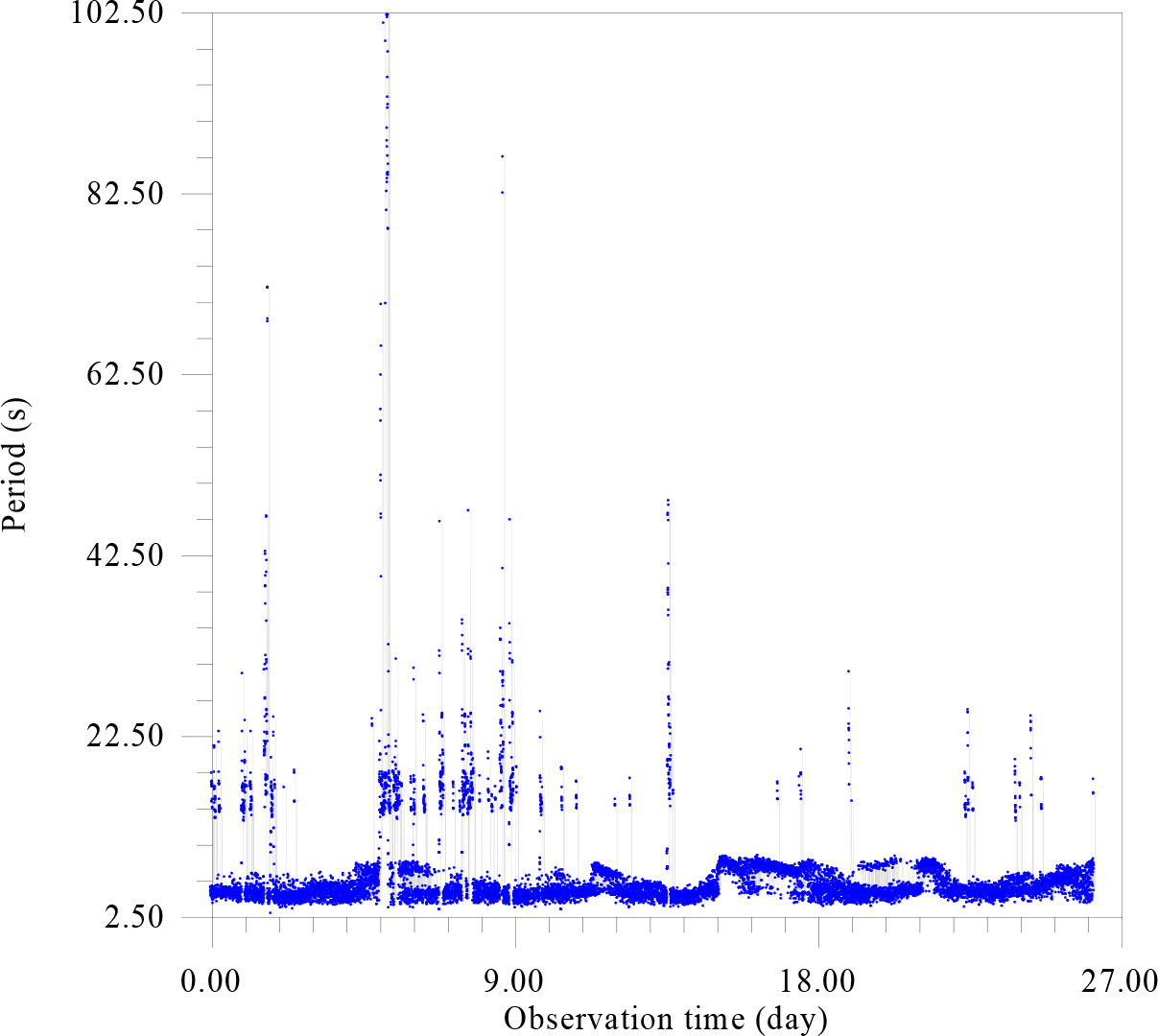
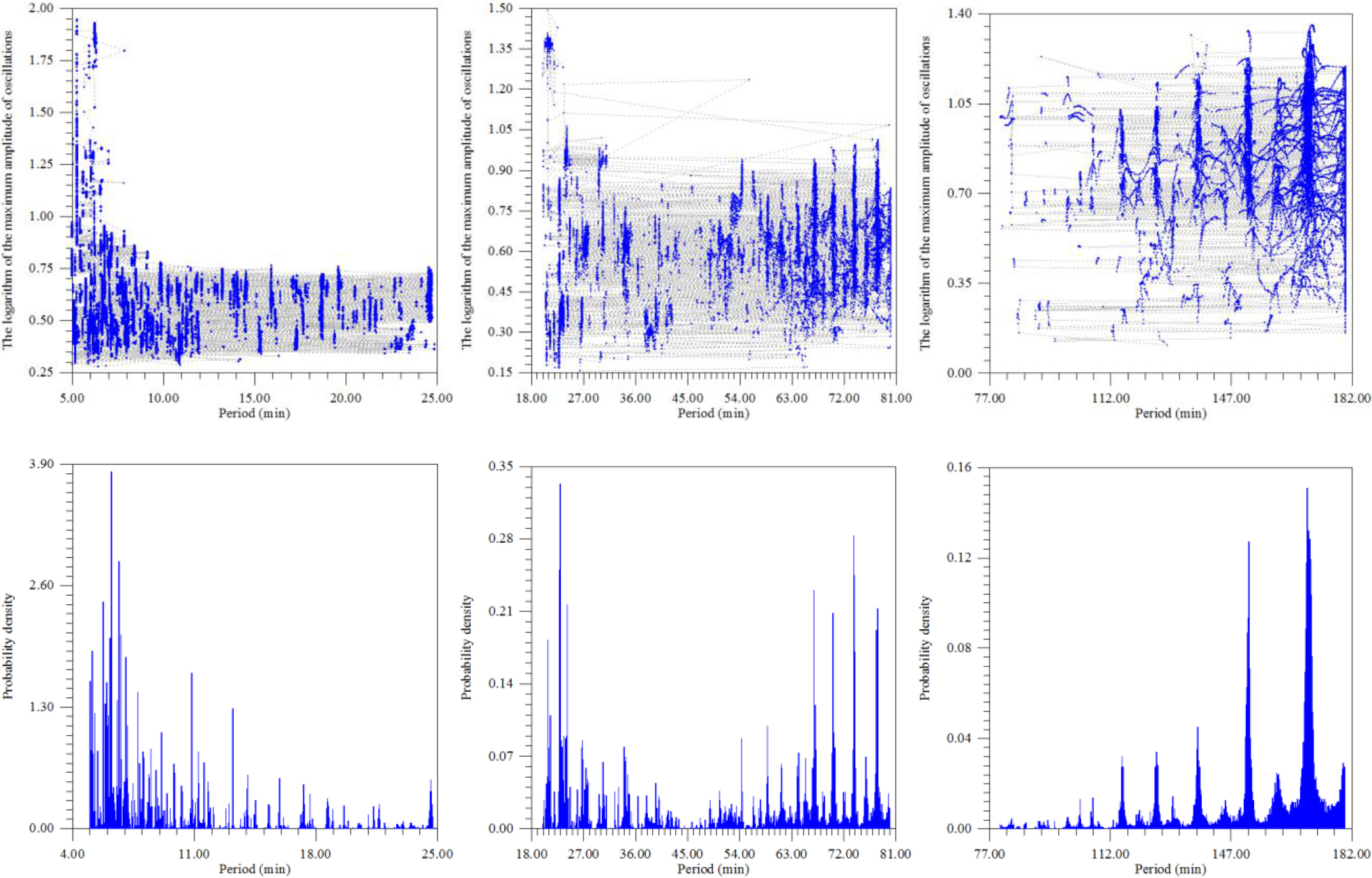
Figure 10. The dependence of the period corresponding to the logarithm of the maximum amplitude of oscillations from the time of observation.
The dependence of the logarithm of the maximum amplitude on the period (Fig. 11) most clearly highlights the zone 3.0 – 7–8.0 s, that is, a known section of storm microseisms. Since such habitual microseisms are usually recorded, for example, in the Baltic and in Europe, and the geological and structural environment of this region and the Antarctic are fundamentally different, a source of probable general influence should be found. Since high-frequency solar oscillations have a constant activity, especially at periods of 5–6 min, and the lack of ozone protection from the Sun allows for higher frequency effects, these microseisms are inherently strongly associated with solar activity. Another, even more active area lies within 20–25 seconds, which is also recorded in other regions of the Earth (Figure-12).
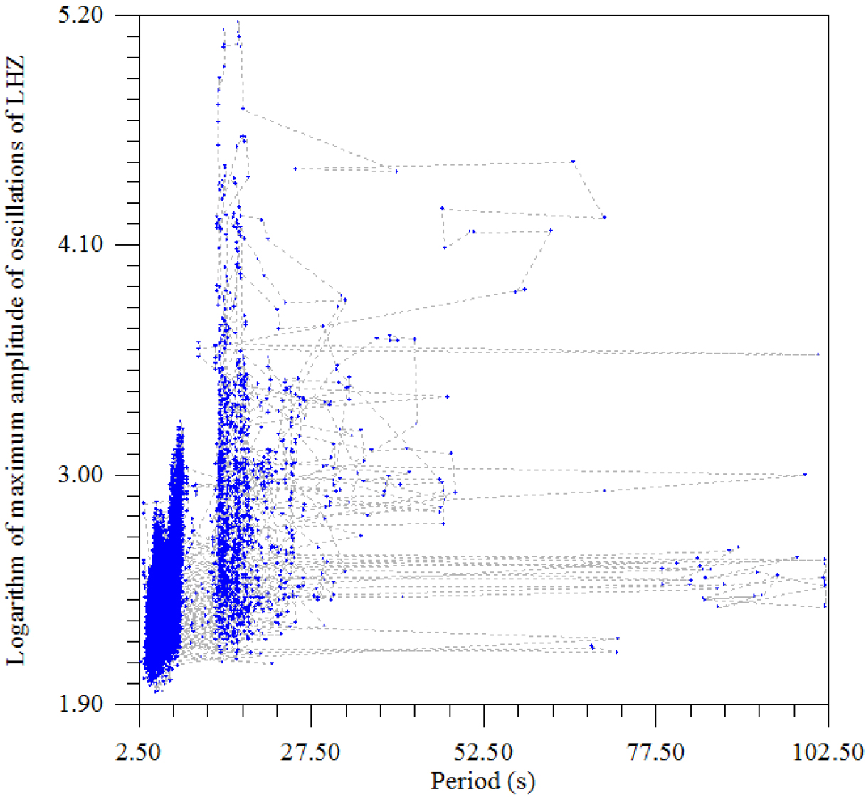
Figure 11. The dependence of the logarithm of the maximum amplitude of oscillations on the period.
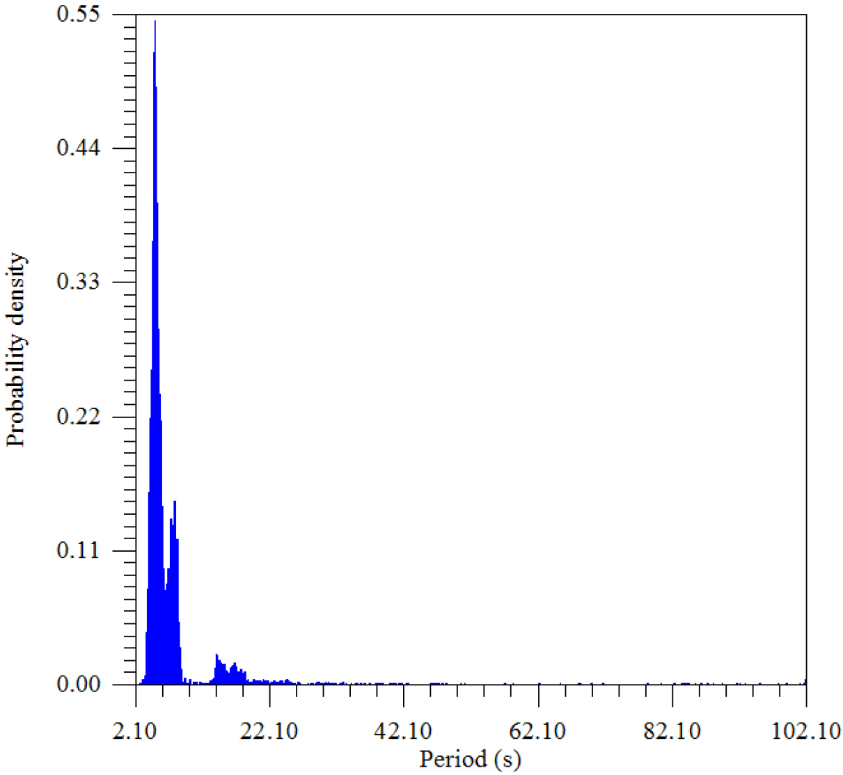
Figure 12. The density distribution of the maximum amplitude of the period.
The distribution of the maximum amplitude over periods divides the seismic vibrations into two groups – powerful ~ 3–6 sec and weak, but connected as resonant harmonics ~ 18–20 sec., which was observed earlier in other regions of the Earth (Figure 13–20).
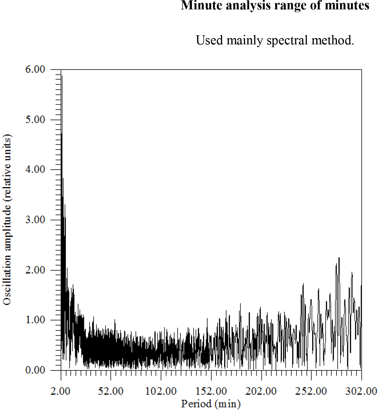
Figure 13. There is amplitude spectrum from 2 to 302 min with a step of 0.03 min.
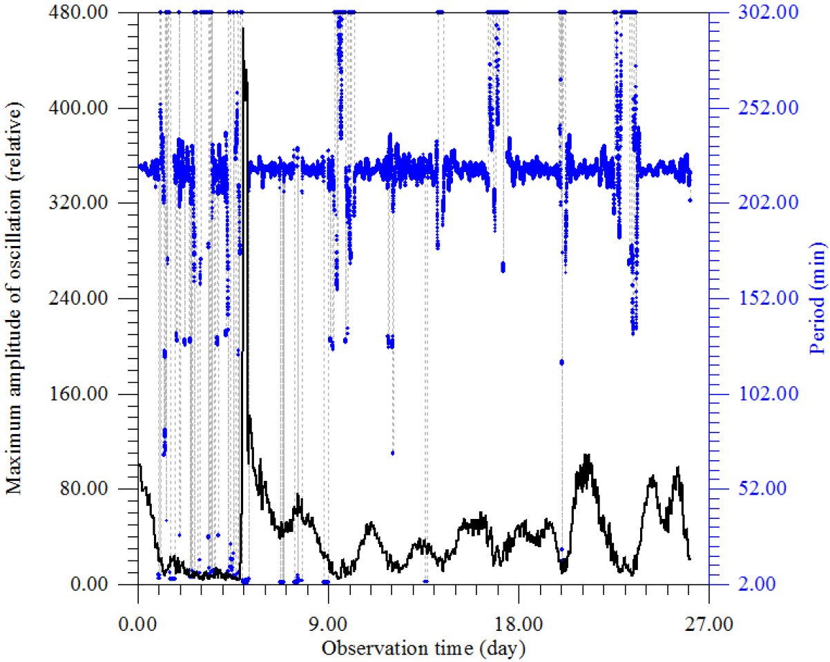
Figure 14. The dependence of the period corresponding to the maximum amplitude of oscillations from the time of observation.
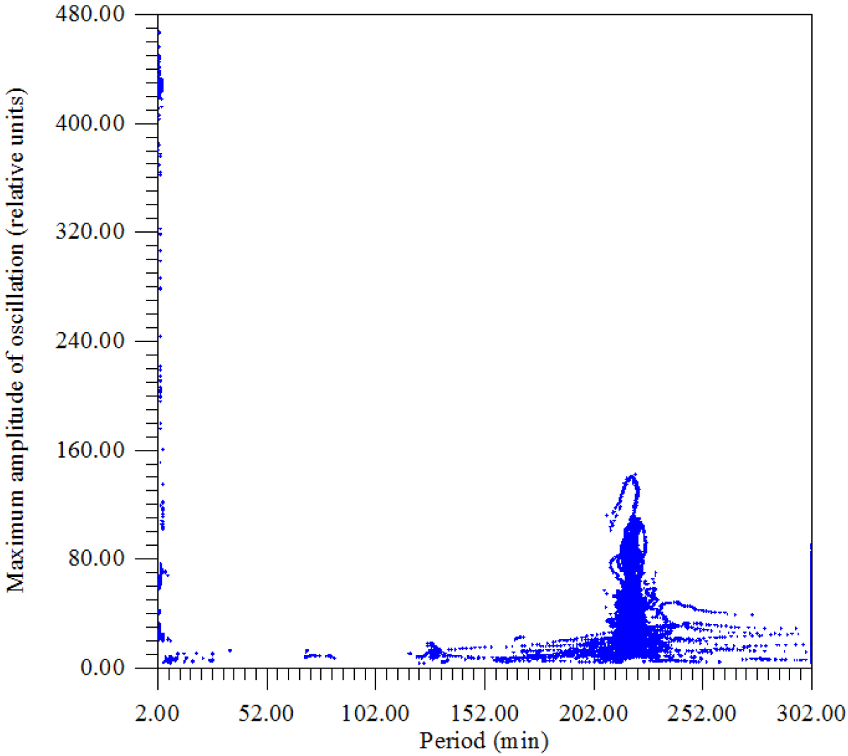
Figure 15. Dependence of the logarithm of the maximum amplitude of oscillations on the period
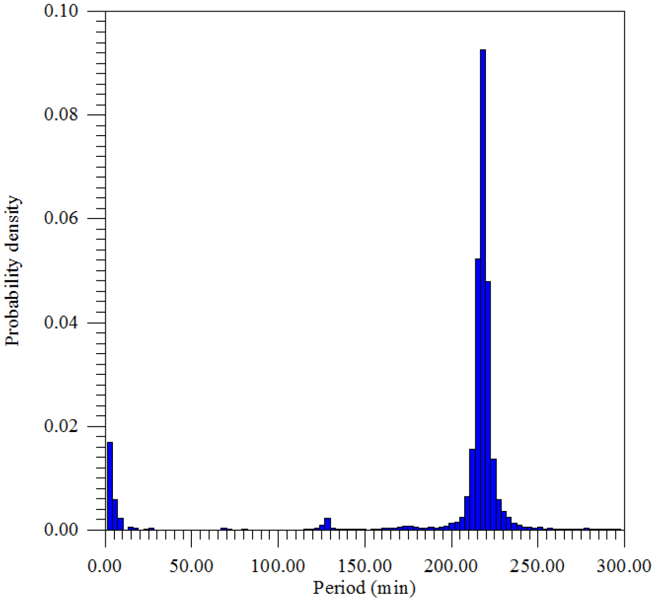
Figure 16. The density distribution of the maximum amplitude of the period.
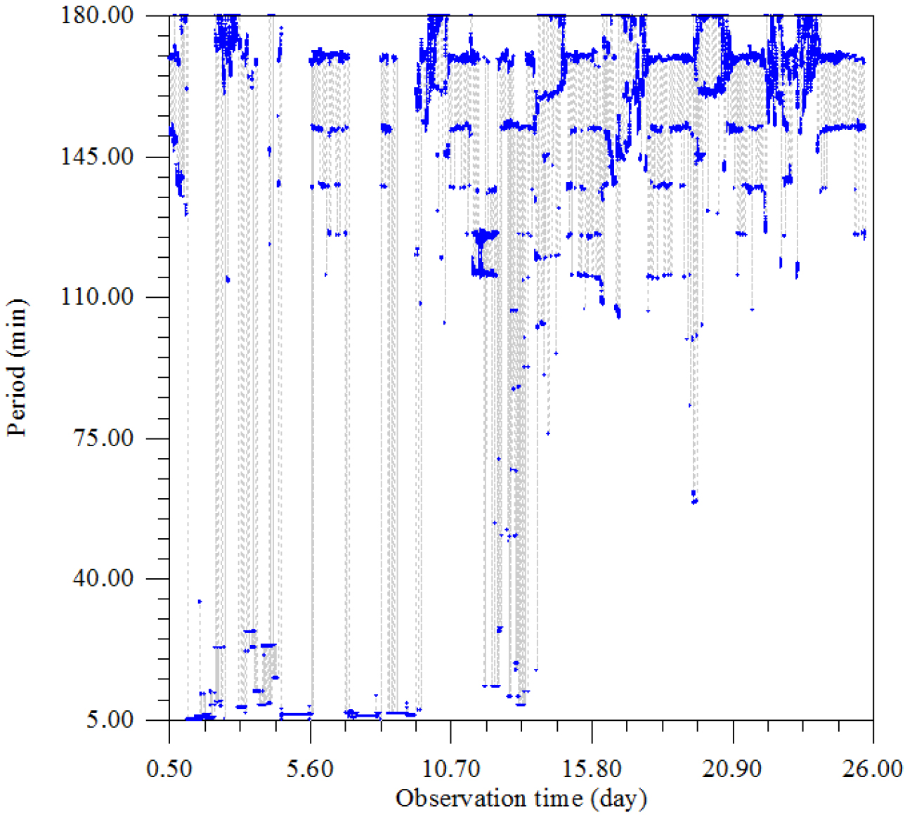
Figure 17. The dependence of the period corresponding to the maximum amplitude of oscillations from the time of observation.
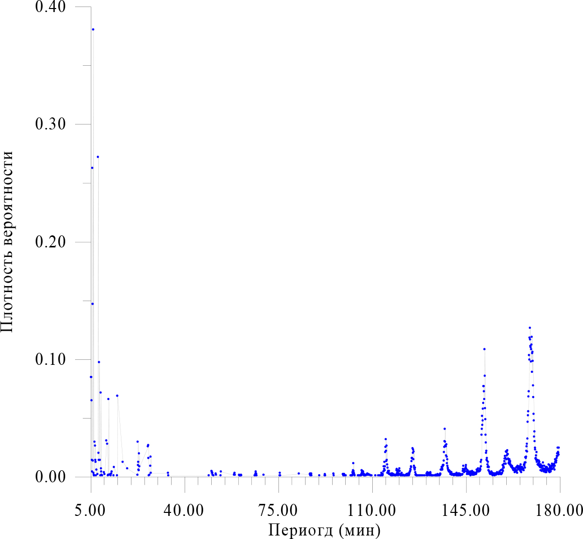
Figure 18. The density distribution of the maximum amplitude of the period.
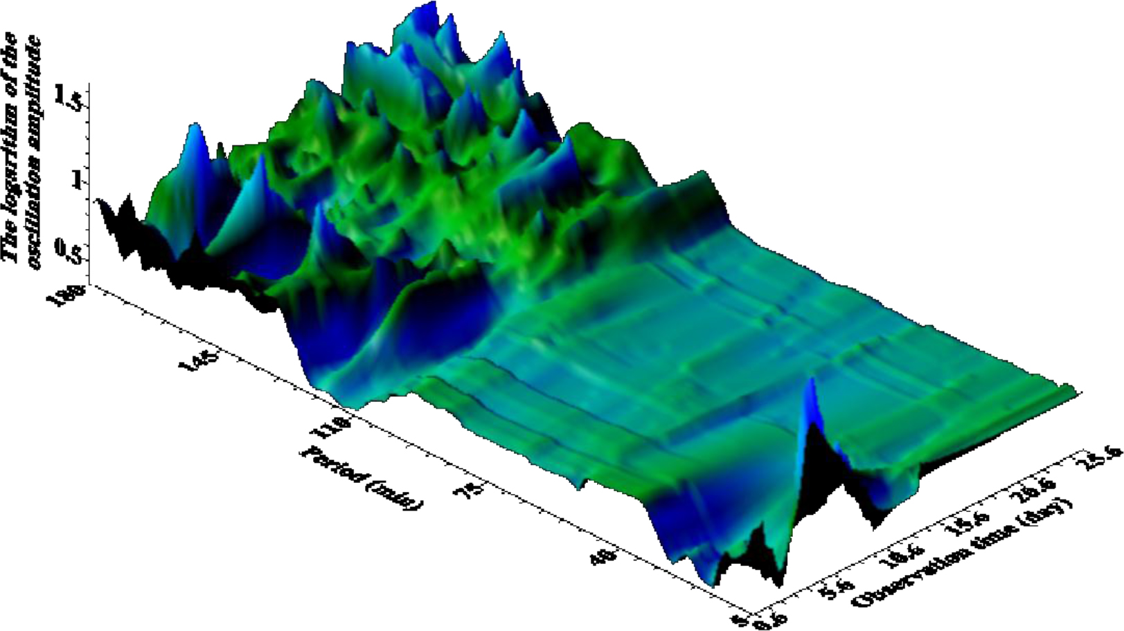
Figure 19. The dependence of the logarithm of the maximum amplitude of oscillations on the time of observation and the corresponding period. The interval of the period is change from 2 to 302 minutes. in 0.3 min steps Time step 2 min. Window – 314 minutes.
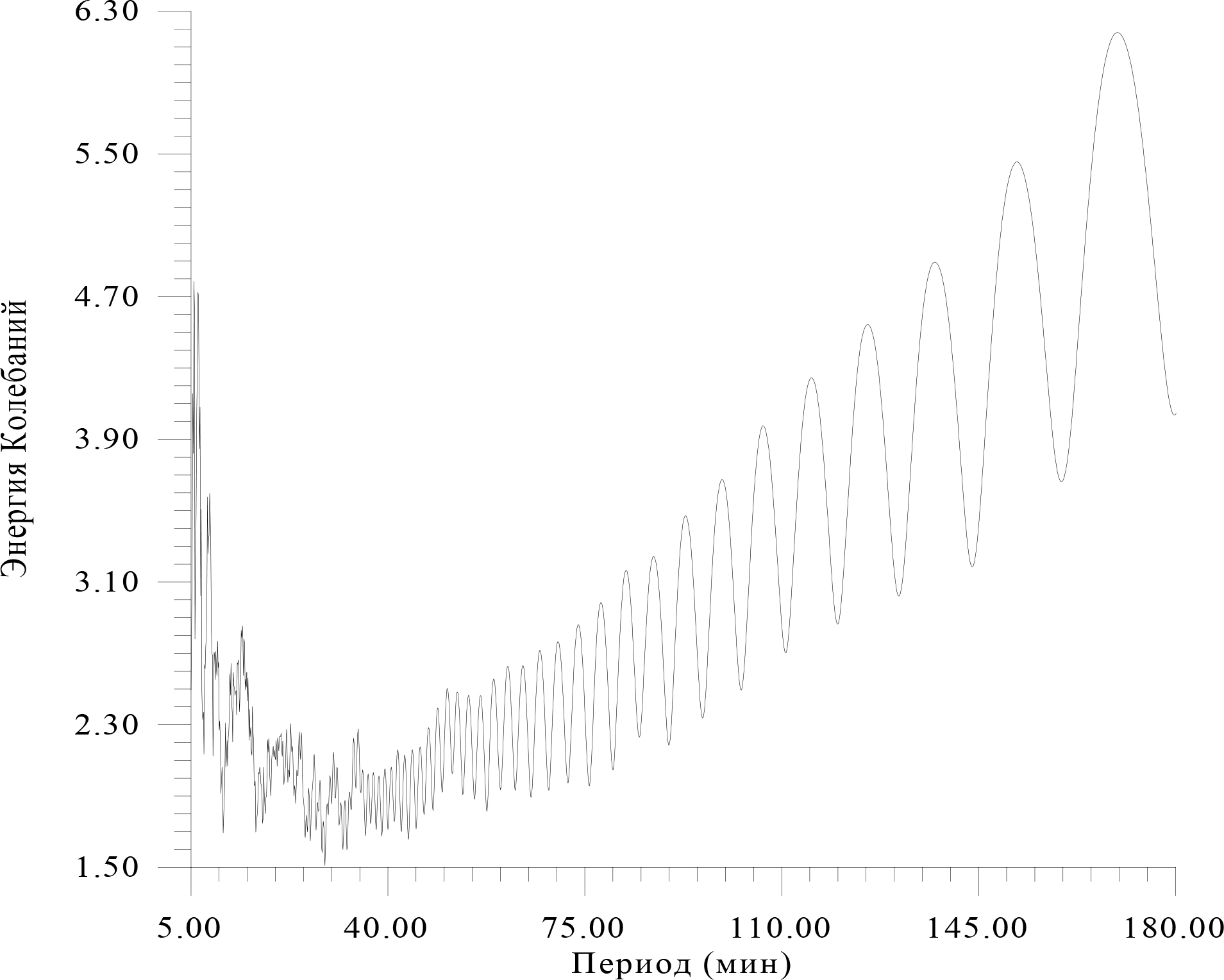
Figure 20. There is energy spectrum data Figure 19.
This energy spectrum characterizes the constant component. Therefore, it is still early to draw final conclusions about their reliability and significance. We must try to modify the program a bit, or use the resonance method (Table-2).
Table 2. Distribution of time intervals for which the periods correspond (N≥10)
|
Period (min) |
N |
Period (min) |
N |
Period (min) |
N |
Period (min) |
N |
Period (min) |
N |
Period (min) |
N |
|
5.4002 |
153 |
124.5683 |
11 |
149.7827 |
12 |
161.0891 |
26 |
167.6929 |
30 |
173.1961 |
18 |
|
5.5003 |
153 |
124.6683 |
10 |
150.5831 |
12 |
161.1892 |
20 |
167.7930 |
39 |
173.2961 |
16 |
|
5.6003 |
117 |
124.7684 |
15 |
150.6832 |
10 |
161.2893 |
25 |
167.8930 |
46 |
173.3962 |
13 |
|
5.7004 |
25 |
124.8685 |
14 |
150.7833 |
22 |
161.3893 |
22 |
167.9931 |
50 |
173.5963 |
15 |
|
5.9005 |
476 |
124.9685 |
23 |
150.8833 |
15 |
161.4894 |
26 |
168.0931 |
38 |
173.6963 |
15 |
|
6.0006 |
266 |
125.0686 |
28 |
150.9834 |
25 |
161.5894 |
18 |
168.1932 |
58 |
173.7964 |
10 |
|
6.1006 |
24 |
125.1686 |
28 |
151.0834 |
64 |
161.6895 |
21 |
168.2933 |
84 |
173.8965 |
16 |
|
6.2007 |
690 |
125.2687 |
27 |
151.1835 |
73 |
161.7895 |
23 |
168.3933 |
94 |
173.9965 |
21 |
|
6.7010 |
53 |
125.3687 |
43 |
151.2835 |
93 |
161.8896 |
18 |
168.4934 |
100 |
174.0966 |
12 |
|
6.9011 |
47 |
125.4688 |
36 |
151.3836 |
79 |
161.9897 |
16 |
168.5934 |
123 |
174.1966 |
11 |
|
7.0011 |
25 |
125.5689 |
41 |
151.4837 |
86 |
162.0897 |
16 |
168.6935 |
131 |
174.4968 |
16 |
|
7.1012 |
22 |
125.6689 |
26 |
151.5837 |
104 |
162.1898 |
14 |
168.7935 |
187 |
174.5969 |
11 |
|
7.4014 |
10 |
125.7690 |
38 |
151.6838 |
113 |
162.2898 |
16 |
168.8936 |
180 |
174.9971 |
11 |
|
8.0017 |
493 |
125.8690 |
16 |
151.7838 |
139 |
162.3899 |
16 |
168.9937 |
214 |
175.0971 |
14 |
|
8.2018 |
36 |
125.9691 |
13 |
151.8839 |
139 |
162.4899 |
15 |
169.0937 |
229 |
175.3973 |
14 |
|
8.3019 |
25 |
126.0691 |
12 |
151.9839 |
131 |
162.5900 |
12 |
169.1938 |
211 |
175.5974 |
10 |
|
8.4019 |
176 |
126.1692 |
10 |
152.0840 |
119 |
162.6901 |
13 |
169.2938 |
201 |
175.6975 |
12 |
|
8.7021 |
25 |
126.2693 |
13 |
152.1841 |
196 |
162.7901 |
12 |
169.3939 |
199 |
175.7975 |
10 |
|
9.0023 |
129 |
135.8747 |
10 |
152.2841 |
155 |
162.8902 |
10 |
169.4939 |
177 |
175.8976 |
10 |
|
9.1023 |
12 |
135.9748 |
10 |
152.3842 |
105 |
163.0903 |
10 |
169.5940 |
196 |
175.9977 |
11 |
|
11.1035 |
55 |
136.0749 |
10 |
152.4842 |
88 |
163.1903 |
12 |
169.6941 |
203 |
176.0977 |
18 |
|
11.4037 |
50 |
136.1749 |
14 |
152.5843 |
64 |
163.2904 |
10 |
169.7941 |
215 |
176.3979 |
17 |
|
11.9039 |
119 |
136.2750 |
10 |
152.6843 |
52 |
163.3905 |
11 |
169.8942 |
161 |
176.5980 |
14 |
|
13.9051 |
14 |
136.3750 |
12 |
152.7844 |
36 |
163.6906 |
10 |
169.9942 |
190 |
176.6981 |
12 |
|
15.2058 |
124 |
136.4751 |
10 |
152.8845 |
39 |
163.9908 |
13 |
170.0943 |
192 |
176.7981 |
14 |
|
17.2070 |
22 |
136.5751 |
15 |
152.9845 |
25 |
164.1909 |
14 |
170.1943 |
178 |
176.9982 |
10 |
|
18.9079 |
12 |
136.6752 |
17 |
153.0846 |
28 |
164.4911 |
16 |
170.2944 |
140 |
177.0983 |
14 |
|
22.8102 |
53 |
136.7753 |
17 |
153.1846 |
24 |
164.5911 |
13 |
170.3945 |
122 |
177.1983 |
16 |
|
22.9102 |
17 |
136.8753 |
17 |
153.2847 |
18 |
164.6912 |
12 |
170.4945 |
96 |
177.2984 |
11 |
|
23.0103 |
22 |
136.9754 |
24 |
153.3847 |
14 |
164.7913 |
13 |
170.5946 |
86 |
177.3985 |
19 |
|
23.1103 |
10 |
137.0754 |
37 |
153.4848 |
22 |
164.8913 |
11 |
170.6946 |
61 |
177.4985 |
11 |
|
23.2104 |
9 |
137.1755 |
45 |
153.5849 |
15 |
164.9914 |
13 |
170.7947 |
69 |
177.5986 |
17 |
|
23.3105 |
35 |
137.2755 |
54 |
153.7850 |
14 |
165.0914 |
15 |
170.8947 |
54 |
177.6986 |
16 |
|
23.4105 |
15 |
137.3756 |
73 |
158.6878 |
10 |
165.1915 |
10 |
170.9948 |
44 |
177.7987 |
17 |
|
26.6123 |
46 |
137.4757 |
53 |
158.8879 |
10 |
165.2915 |
12 |
171.0949 |
41 |
177.8987 |
17 |
|
26.7124 |
48 |
137.5757 |
47 |
158.9879 |
17 |
165.3916 |
15 |
171.1949 |
27 |
177.9988 |
13 |
|
26.8125 |
28 |
137.6758 |
47 |
159.1881 |
13 |
165.4917 |
12 |
171.2950 |
28 |
178.0989 |
17 |
|
27.5129 |
16 |
137.7758 |
46 |
159.2881 |
15 |
165.6918 |
18 |
171.3950 |
32 |
178.1989 |
19 |
|
27.6129 |
30 |
137.8759 |
32 |
159.3882 |
13 |
165.7918 |
10 |
171.4951 |
25 |
178.2990 |
10 |
|
103.2561 |
20 |
137.9759 |
49 |
159.4882 |
19 |
165.9919 |
13 |
171.5951 |
37 |
178.3990 |
16 |
|
114.5626 |
15 |
138.0760 |
30 |
159.5883 |
23 |
166.0920 |
14 |
171.6952 |
22 |
178.4991 |
26 |
|
114.7627 |
11 |
138.1761 |
20 |
159.6883 |
27 |
166.1921 |
14 |
171.7953 |
23 |
178.5991 |
22 |
|
114.8627 |
22 |
138.2761 |
26 |
159.7884 |
31 |
166.2921 |
10 |
171.8953 |
25 |
178.6992 |
25 |
|
115.0629 |
15 |
138.3762 |
16 |
159.8885 |
19 |
166.3922 |
11 |
171.9954 |
18 |
178.7993 |
23 |
|
115.1629 |
37 |
138.4762 |
13 |
159.9885 |
28 |
166.4922 |
12 |
172.0954 |
24 |
178.8993 |
21 |
|
115.2630 |
45 |
138.5763 |
11 |
160.0886 |
19 |
166.5923 |
10 |
172.1955 |
24 |
178.9994 |
24 |
|
115.3630 |
57 |
144.1795 |
11 |
160.1886 |
38 |
166.6923 |
12 |
172.2955 |
17 |
179.0994 |
28 |
|
115.4631 |
39 |
144.2795 |
16 |
160.2887 |
26 |
166.8925 |
18 |
172.3956 |
20 |
179.1995 |
31 |
|
115.5631 |
23 |
144.4797 |
10 |
160.3887 |
37 |
166.9925 |
16 |
172.4957 |
24 |
179.2995 |
35 |
|
115.6632 |
47 |
144.9799 |
11 |
160.4888 |
32 |
167.0926 |
18 |
172.5957 |
16 |
179.3996 |
31 |
|
115.7633 |
25 |
145.0800 |
12 |
160.5889 |
39 |
167.1926 |
21 |
172.6958 |
22 |
179.4997 |
44 |
|
115.8633 |
18 |
145.1801 |
14 |
160.6889 |
40 |
167.2927 |
13 |
172.7958 |
15 |
179.5997 |
37 |
|
116.0634 |
13 |
145.2801 |
17 |
160.7890 |
34 |
167.3927 |
29 |
172.8959 |
14 |
179.6998 |
36 |
|
119.4654 |
11 |
145.3802 |
11 |
160.8890 |
34 |
167.4928 |
21 |
172.9959 |
18 |
179.7998 |
33 |
|
120.4659 |
12 |
149.2824 |
10 |
160.9891 |
27 |
167.5929 |
28 |
173.0960 |
9 |
179.8999 |
44 |
This table could also be rebuilt according to a different number of intervals by period. It is noteworthy that in the range of 28÷103 min the number of intervals is very small (Table 3) (Figure 21) (Table 4).
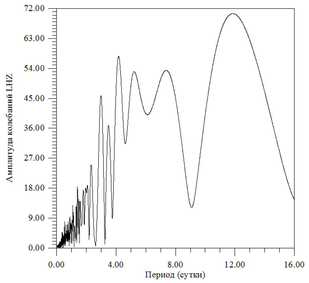
Figure 21. There is amplitude spectrum of the daily range.
Table 3. The distribution of time intervals for which the periods correspond to Amax
|
Period (min) |
N |
Period (min) |
N |
Period (min) |
N |
|
2.6000 |
946 |
146.3120 |
4 |
221.1620 |
2686 |
|
5.5940 |
325 |
149.3060 |
4 |
224.1560 |
762 |
|
8.5880 |
122 |
152.3000 |
1 |
227.1500 |
332 |
|
11.5820 |
1 |
155.2940 |
9 |
230.1440 |
196 |
|
14.5760 |
30 |
158.2880 |
13 |
233.1380 |
140 |
|
17.5700 |
15 |
161.2820 |
18 |
236.1320 |
71 |
|
20.5640 |
1 |
164.2760 |
17 |
239.1260 |
54 |
|
23.5580 |
9 |
167.2700 |
25 |
242.1200 |
36 |
|
26.5520 |
20 |
170.2640 |
36 |
245.1140 |
36 |
|
32.5400 |
2 |
173.2580 |
42 |
248.1080 |
24 |
|
68.4680 |
17 |
176.2520 |
44 |
251.1020 |
31 |
|
71.4620 |
6 |
179.2460 |
26 |
254.0960 |
13 |
|
74.4560 |
2 |
182.2400 |
20 |
257.0900 |
15 |
|
77.4500 |
2 |
185.2340 |
18 |
260.0840 |
10 |
|
80.4440 |
7 |
188.2280 |
33 |
263.0780 |
10 |
|
116.3720 |
3 |
191.2220 |
22 |
266.0720 |
9 |
|
119.3660 |
6 |
194.2160 |
35 |
269.0660 |
7 |
|
122.3600 |
15 |
197.2100 |
47 |
272.0600 |
11 |
|
125.3540 |
48 |
200.2040 |
71 |
275.0540 |
11 |
|
128.3480 |
128 |
203.1980 |
86 |
278.0480 |
17 |
|
131.3420 |
19 |
206.1920 |
135 |
281.0420 |
10 |
|
134.3360 |
14 |
209.1860 |
359 |
284.0360 |
5 |
|
137.3300 |
5 |
212.1800 |
868 |
287.0300 |
7 |
|
140.3240 |
4 |
215.1740 |
2932 |
290.0240 |
3 |
|
143.3180 |
6 |
218.1680 |
5189 |
293.0180 |
6 |
|
|
|
|
|
296.0120 |
6 |
Table 4. The summary of daily periods.
|
Period |
Amplitude |
Period |
Amplitude |
Period |
Amplitude |
|
0.00417 |
2.19146 |
0.38750 |
2.34914 |
0.79306 |
7.95374 |
|
0.00972 |
1.39646 |
0.39861 |
3.12503 |
0.82917 |
4.96194 |
|
0.11806 |
1.05268 |
0.40694 |
4.69761 |
0.88750 |
9.37318 |
|
0.13194 |
1.14954 |
0.41806 |
2.71686 |
0.93750 |
7.53833 |
|
0.13750 |
1.06967 |
0.42917 |
2.80484 |
0.97639 |
7.36167 |
|
0.16806 |
1.43672 |
0.43750 |
3.39350 |
1.04583 |
8.34664 |
|
0.18750 |
1.28783 |
0.44583 |
3.64884 |
1.09583 |
12.86868 |
|
0.20139 |
1.51607 |
0.46250 |
1.25450 |
1.15139 |
9.73151 |
|
0.20972 |
1.87710 |
0.47083 |
3.53236 |
1.20972 |
6.42397 |
|
0.22083 |
1.91259 |
0.48750 |
3.70950 |
1.31806 |
12.39736 |
|
0.22917 |
2.03499 |
0.50417 |
2.77930 |
1.40139 |
18.42374 |
|
0.24028 |
2.07343 |
0.51528 |
3.61388 |
1.49028 |
14.78352 |
|
0.25139 |
1.51939 |
0.52917 |
6.31336 |
1.59306 |
14.11028 |
|
0.26528 |
1.78014 |
0.54028 |
7.88273 |
1.79306 |
17.42602 |
|
0.28194 |
1.69116 |
0.55417 |
3.96956 |
1.95972 |
18.00527 |
|
0.29306 |
1.73287 |
0.56528 |
1.75607 |
2.07917 |
18.77936 |
|
0.29861 |
2.50799 |
0.57639 |
1.94631 |
2.32639 |
25.01781 |
|
0.30972 |
2.22962 |
0.59028 |
4.55191 |
2.99028 |
45.80661 |
|
0.31528 |
2.12205 |
0.60694 |
6.98497 |
3.49583 |
36.81036 |
|
0.32917 |
2.22865 |
0.62361 |
4.12886 |
4.17083 |
57.67608 |
|
0.33472 |
3.07918 |
0.64861 |
3.80290 |
5.22083 |
52.97682 |
|
0.35139 |
2.24693 |
0.66806 |
3.72560 |
7.37917 |
53.38868 |
|
0.35694 |
4.71118 |
0.68750 |
6.98646 |
11.85972 |
70.47160 |
|
0.37361 |
2.58232 |
0.71528 |
4.98707 |
|
|
|
0.38194 |
3.51410 |
0.76250 |
7.11657 |
|
|
Conclusion
As expected, (see Tables 2–4), the structure of the seismic fields of Antarctica is saturated with wave fields determined by cosmic processes, primarily by the Sun’s own oscillations (see Table 1). Seismic Antarctica turns it into a unique and indispensable landfill for testing and testing of seismic and geophysical equipment intended for the study of the Moon and planets.
Attachments
References
- Khavroshkin OB, Tsyplakov VV (2001) Meteoroid stream impacts on the Moon: information of duration of seismograms // Proc. Conf. Meteoroids 2001 (ESA SP-495). Noordwijk, The Netherlands: ESA Publ Division Pg No: 13–21.
- Khavroshkin OB, Tsyplakov VV (2001) Temporal structure of meteoroid stream and lunar seismicity according to Nakamura’s catalogue // Proc. Conf. Meteoroids 2001 (ESA SP-495). Noordwijk, The Netherlands: ESA Publ. Division Pg No: 95–105.
- Khavroshkin OB, Tsyplakov VV, Sobko AA (2011) Solar activity and seismicity of the Moon. Engineering Physics 3: 40–45.
- Christensen Dalsgaard J, Gough DO, Morgan JG (1979) Dirty Solar Models. Astron. Astrophys 73: 121–128 .
- Patrick S. McIntosh, Murray Dryer (1972) Solar activity: observations and predictions. The Massachusetts Institute of Technology, Virginia, USA.
- Syun-Ichi Akasofu, Sydney Chapman (1972) Solar-Terrestrial Physics. The Clarendon Press, California, USA.
- Khavroshkin O, Tsyplakov V (2013) Nonlinear Seismology: The Cosmic Component. Saarbrücken: Palmarium Academic Publishing.
- Oleg Khavroshkin, Vladislav Tsyplakov (2013) Sun, Earth, radioactive ore: common periodicity. The Natural Science (NS) 5: 1001–1005.
- Khavroshkin OB, Tsyplakov VV (2013) Radioactivity, solar neutrinos, interactions. Engineering Physics 8: 53–61.
- Khavroshkin OB, Tsyplakov VV (2013) Ore sample radioactivity: monitoring. Engineering Physics 8: 53–62.
- Khavroshkin OB, Tsyplakov VV (2013) Natural radioactivity as an open system. Engineering Physics 12: 40–54.
- Starodubov AV, Khavroshkin OB, Tsyplakov VV (2014) From periodicities of radioactivity to cosmic and metaphysical oscillations. Metaphysics. Moscow. Peoples’ Friendship University of Russia 1: 137–149.
- Rukhadze AA, Khavroshkin OB, Tsyplakov VV (2015) The frequency of natural radioactivity. Engineering Physics 5.
- Khavroshkin OB, Tsyplakov VV (2014) Hydrogen maser: solar periodicity. Engineering Physics 3: 25–31.