Abstract
In recent years, the use of a two-stage seamless adaptive design in clinical research has become popular, which combines two separate clinical studies into a single study that can address the study objectives of two separate studies. The design cannot only reduce the lead time between the two separate trials and consequently shorten the development process, but also increase the probability of success of the intended clinical trial because critical decisions or adaptations can be made after the review of interim data at the end of the first stage. Depending on study objectives, study endpoints, and target patient populations at different stages, two-stage seamless adaptive designs can be classified into “k-D” designs (k is the number of different dimensions). A primary assumption that the study endpoint at the first stage is predictive of the study endpoint at the second stage, consideration of using two sets of hypotheses to account for different study objectives at different stages, and an assessment of a sensitivity index for possible population shifts are proposed for valid statistical analyses for a given type of “k-D” design. Examples concerning a hepatitis C virus (HCV) infection clinical study and a non-alcoholic steatohepatitis (NASH) clinical trial are presented.
Keywords
Two-stage phase 1/2 (2/3) seamless adaptive design; The “k-D” design; Population shift; NASH clinical trial
Introduction
In recent years, the use of seamless adaptive designs in clinical trials has become very popular in clinical research and development. A seamless trial design is defined as a design that combines two separate (independent) trials into a single study [1]. The single study is able to address the study objectives that are normally achieved through the conduct of the two trials. An adaptive seamless trial design is referred to as a seamless design that applies adaptations during the conduct of the trial. A seamless adaptive design would use data collected from patients enrolled before and after the adaptation in the final analysis. A typical example is a two-stage phase 2/3 seamless adaptive clinical trial which consists of two stages, namely a learning (or exploratory) stage (e.g., phase 2 for dose finding or drop the lowers) and a confirmatory stage (e.g., phase 3 study for efficacy confirmation). See also, EMA (2014) [2]; FDA (2019). A two-stage seamless adaptive trial design has the following characteristics: (i) it combines two separate and independent trials into a single trial, (ii) the single trial consists of two stages, namely a learning (exploratory) stage and a confirmatory stage, and (iii) it offers opportunities for adaptations based on accrued data at the end of learning stage [3]. A two-stage seamless adaptive design provides an opportunity for saving because it allows stopping a trial early for safety and/or futility/efficacy. In addition, it can reduce the lead time between the learning stage and the confirmatory stage. Furthermore, data collected at the learning stage can be combined with those data obtained at the confirmatory stage for a final analysis for obtaining a more accurate and reliable assessment of the treatment effect under study. However, the use of a two-stage seamless adaptive trial design also suffers from the following limitations (or regulatory concerns): (i) it may introduce operational bias (e.g., adaptations relate to dose, hypothesis, and endpoint, etc), (ii) it may not be able to control the overall type I error rate, (iii) statistical methods for combined analysis are not well established especially when the study objectives and study endpoints are different at different stages, and (iv) the complexity of the two-stage seamless adaptive design depends upon the adaptations apply [4,5]. Depending upon whether the study objectives, study endpoints, and target populations at different stages are the same, two-stage seamless adaptive designs can be classified into several categories. Statistical methods for data analysis including power calculation for sample size calculation and allocation are different for seamless adaptive designs in different categories. In the next section, these types of seamless adaptive designs are defined. Section 3 describes the analysis methods of these types of seamless adaptive clinical trials with one or more differences in study objective, endpoint, and/or target patient population. Section 4 discusses primary assumptions and statistical considerations for analysis of a general “K-D” design”. Two examples concerning a hepatitis C virus (HCV) infection clinical study and a non-alcoholic steatohepatitis (NASH) clinical trial are presented to illustrate the application of a “2- D” design and a “3-D” design, respectively. Some concluding remarks are given in the last section of this article.
Types of Two-Stage Seamless Adaptive Design
Generally, a seamless adaptive design has three key dimensions: study objective, study endpoint, and target patient population. As is described in Table 1, in practice, a seamless adaptive design may combine two separate (independent) trials with similar but different study objectives into a single trial, e.g., a phase 2 trial for dose selection and a phase 3 study for efficacy confirmation. In addition, the study endpoints considered at the two separate trials may be different, e.g., a biomarker or surrogate endpoint versus a regular clinical endpoint. In some cases, such as non-alcoholic steatohepatitis (NASH) clinical trials, the target patient populations may have been shifted due to disease progression at different stages (e.g., fibrosis, cirrhosis, and liver transplant). Thus, the three dimensions may be the same or different in a particular two stage seamless adaptive design. We can classify two-stage seamless adaptive designs into eight categories depending upon whether the study objectives, study endpoints, and target patient populations at different stages are the same (Table 2).
Table 1: Three Key Dimensions of a Seamless Adaptive Design.
|
Dimension |
Example |
| Study objective | Dose selection versus efficacy confirmation |
| Study endpoint | A biomarker or surrogate endpoint versus a regular clinical endpoint |
| Target patient population | It may be shifted due to disease progression at different stages (e.g., fibrosis, cirrhosis, and liver transplant). |
Table 2: Types of Two-Stage Seamless Adaptive Designs (Depending upon Objective, Endpoint, and Target Population)
|
Study Objective |
Target Patient Population | |||
|
Same (S) |
Different (D) | |||
| Study Endpoint |
Study Endpoint |
|||
| Same (S) | Different (D) | Same (S) |
Different (D) |
|
| Same (S) |
SSS |
SDS | SSD |
SDD |
| Different (D) |
DSS |
DDS | DSD |
DDD |
Table 3 indicates that there is one “0-D design”, three “1-D design”, three “2-D design”, and one “3-D design”. These “K-D” designs, where K is the number of differences in objective, endpoint, and target patient population are briefly described below.
The “0-D” design is a two-stage seamless adaptive design with the same study objective and same study endpoint at different stages under the same target patient population, which is similar to typical group sequential design with a planned interim analysis.
For the “1-D” designs, there are three different types: (i) the study objective is different at different stages (e.g., dose selection versus efficacy confirmation), (ii) the study endpoint is different at different stages (e.g., biomarker or surrogate endpoint or clinical endpoint with shorter duration versus clinical endpoint), and (iii) the target patient population is different at different stages (e.g., population shift before and after adaptations applied based on the review of interim analysis at the end of the first stage).
For the “2-D” designs, there are three different types: (i) both study objective and endpoint are different at different stages (e.g., dose selection versus efficacy confirmation and biomarker or surrogate endpoint or clinical endpoint with shorter duration versus clinical endpoint), (ii) both study objective and target patient population are different at different stages (e.g., dose selection versus efficacy confirmation and population shift before and after adaptations applied based on the review of interim analysis at the end of the first stage), and (iii) both study endpoint and the target patient population are different at different stages (e.g., biomarker or surrogate endpoint or clinical endpoint with shorter duration versus clinical endpoint and population shift before and after adaptations applied based on the review of interim analysis at the end of the first stage).
For the “3-D” designs, in addition to differences in study objective and study endpoint at different stages, the target patient population is also different at different stages. A typical example is a two-stage NASH seamless adaptive clinical trial, which will be further discussed in a later section.
Table 3: Types of Two-Stage Seamless Adaptive Designs (Depending upon the Number of Differences in Objective, Endpoint, and Target Population). Depending on the number of differences in study objective, endpoint, and target population, Table 2 can be summarized as the following table.
|
Two-Stage Seamless Design |
|||
| The “0-D” design | The “1-D” design | The “2-D” design |
The “3-D” design |
|
SSS |
DSS |
DDS |
DDD |
|
SDS |
DSD | ||
| SSD |
SDD |
||
Note: S = Same, D = Different
Analysis of Seamless Adaptive Trial Design
Analysis for Seamless Design with Different Objectives
In this section, we will focus on statistical inference for the scenario where the study objectives at different stages are different (e.g., dose selection versus efficacy confirmation) and study endpoints at different stages are different (e.g., biomarker or surrogate endpoint versus regular clinical study endpoint). As indicated earlier, one of the major concerns when applying adaptive design methods in clinical trials is probably how to control the overall type I error rate at a pre-specified level of significance. It is also a concern that how the data collected from both stages should be combined for the final analysis. Besides, it is of interest to know how the sample size calculation/allocation should be done for achieving individual study objectives originally set for the two stages (separate studies). In this article, a multiple-stage transitional seamless trial design with different study objectives and different study endpoints and with and without adaptations is proposed. The impact of the adaptive design methods on the control of the overall type I error rate under the proposed trial design is examined. Valid statistical test and the corresponding formulas for sample size calculation/allocation are derived under the proposed trial design. As indicated earlier, a two- stage seamless trial design that combines two independent studies (e.g., a phase 2 study and a phase 3 study) is often considered in clinical research and development. Under such a trial design, the investigator may be interested in having one planned interim analysis at each stage. In this case, the two-stage seamless trial design becomes a 4-stage trial design if we consider the time point at which the planned interim analysis will be conducted as end of the specific stage. In this article, we will refer to such a trial design as a multiple-stage transitional seamless design to emphasize the importance of smooth transition from stage to stage. In what follows, we will focus on the proposed multiple-stage transitional seamless design with (adaptive version) and without (non- adaptive version) adaptations.
Consider a clinical trial comparing k treatments groups, ![]() with a control group C. One early surrogate endpoint and one subsequent primary endpoint are potentially available for assessing the treatment effect. Let
with a control group C. One early surrogate endpoint and one subsequent primary endpoint are potentially available for assessing the treatment effect. Let ![]() and
and ![]() be the treatment effect comparing
be the treatment effect comparing ![]() with C measured by the surrogate endpoint and the primary endpoint, respectively. The ultimate hypothesis of interest is
with C measured by the surrogate endpoint and the primary endpoint, respectively. The ultimate hypothesis of interest is
![]()
which is formulated in terms of the primary endpoint. However, along the way, the hypothesis
![]()
In terms of the short-term surrogate endpoint will also be assessed. Cheng [1,3] assumed that ![]() is a monotone increasing function of the corresponding
is a monotone increasing function of the corresponding ![]() . The trial is conducted as a group sequential trial with the accrued data analyzed at 3 stages (i.e., stage 1, stage 2a, stage 2b, and stage 3) with 4 interim analyses, which are briefly described below. The timeline of the trial is depicted in Figure 1. For simplicity, consider the case where the variances of the surrogate endpoint and the primary outcomes, denoted as
. The trial is conducted as a group sequential trial with the accrued data analyzed at 3 stages (i.e., stage 1, stage 2a, stage 2b, and stage 3) with 4 interim analyses, which are briefly described below. The timeline of the trial is depicted in Figure 1. For simplicity, consider the case where the variances of the surrogate endpoint and the primary outcomes, denoted as ![]() and
and ![]() are known.
are known.
Figure 1: Timeline of a Seamless Trial of Different Objectives and Different Endpoints with 4 Interim Analyses.
At Stage 1 of the study, (k +1)n1 subjects will be randomized equally to receive either one of the k treatments or the control. As the result, there are n1 subjects in each group. At the first interim analysis, the most promising treatment will be selected and used in the subsequent stages based on the surrogate endpoint. Let  be the pair wise test statistics, and
  , then if
  for some c1, then the trial is stopped and H0,1 is accepted. Otherwise, if
  , then the treatment Esis recommended as the most promising treatment and will be used in all the subsequent stages. Note that only the subjects receiving either the promising treatment or the control will be followed formally for the primary endpoint. The treatment assessment on all other subjects will be terminated and the subjects will receive standard care and undergo necessary safety monitoring.
At Stage 2a, 2n2 , additional subjects will be equally randomized to receive either the treatment Es or the control C. The second interim analysis is scheduled when the short-term surrogate measures from these 2n2 Stage 2 subjects and the primary endpoint measures from those 2n1 Stage 1 subjects who receive either the treatment Es or the control C become available. Let ![]() and
and  be the pairwise test statistics from Stage 1 based on the surrogate endpoint and the primary endpoint, respectively, and
 ![]() be the statistic from Stage 2 based on the surrogate. If
be the statistic from Stage 2 based on the surrogate. If
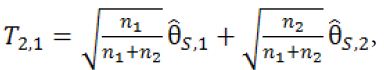
then stop the trial and accept H0,1. If T2.1 > C2.1 and T1.2 > C1.2, then stop the trial and reject both H0,1 and H0,2. Otherwise, if T2.1 > C2.1 but 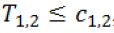 , then we will move on to Stage 2b.
At Stage 2b, no additional subjects will be recruited. The third interim analysis will be performed when the subjects in Stage 2a complete their primary endpoints. Let
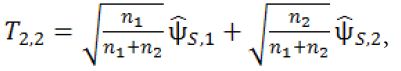
where ![]() is the pair-wise test statistic from stage 2b. If T2.2 > C2.2, then stop the trial and reject H0,2 . Otherwise, we move on to Stage 3.
is the pair-wise test statistic from stage 2b. If T2.2 > C2.2, then stop the trial and reject H0,2 . Otherwise, we move on to Stage 3.
At Stage 3, the final stage, 2n3 additional subjects will be recruited and followed till their primary endpoints. For the fourth interim analysis, define
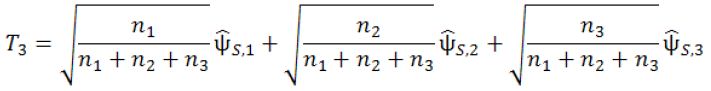
where ![]() is the pair-wise test statistic from stage 3. If T3 > C3, then stop the trial and reject H0,2; otherwise, accept H0,2. The parameters in the above designs, n1, n2, n3, c1.1, c1.2, c2.1, c2.2 and c3 are determined such that the procedure will have a controlled type I error rate of α and a target power of 1−β. The determination of these parameters will be given in next section.
is the pair-wise test statistic from stage 3. If T3 > C3, then stop the trial and reject H0,2; otherwise, accept H0,2. The parameters in the above designs, n1, n2, n3, c1.1, c1.2, c2.1, c2.2 and c3 are determined such that the procedure will have a controlled type I error rate of α and a target power of 1−β. The determination of these parameters will be given in next section.
Analysis for Seamless Design with Different Endpoints
For illustration purpose, consider a two-stage phase 2/3 seamless adaptive trial design with different (continuous) study endpoints. Let ![]() be the observation of one study endpoint (e.g., a biomarker) from the
be the observation of one study endpoint (e.g., a biomarker) from the ![]() subject in phase 2,
subject in phase 2, ![]() 1,…, n and yj be the observation of another study endpoint (the primary clinical endpoint) from the jth subject in phase 3, j=1,…, m. Assume that
1,…, n and yj be the observation of another study endpoint (the primary clinical endpoint) from the jth subject in phase 3, j=1,…, m. Assume that ![]() ‘s are independently and identically distributed with
‘s are independently and identically distributed with ![]() and
and ![]() ; and yj′s are independently and identically distributed with E(yj)=μ and
; and yj′s are independently and identically distributed with E(yj)=μ and ![]() . Chow, Lu (2007) proposed using the established functional relationship to obtain predicted values of the clinical endpoint based on data collected from the biomarker (or surrogate endpoint). Thus, these predicted values can be combined with the data collected at the confirmatory phase to develop a valid statistical inference for the treatment effect under study. Suppose that x and y can be related in a straight-line relationship
. Chow, Lu (2007) proposed using the established functional relationship to obtain predicted values of the clinical endpoint based on data collected from the biomarker (or surrogate endpoint). Thus, these predicted values can be combined with the data collected at the confirmatory phase to develop a valid statistical inference for the treatment effect under study. Suppose that x and y can be related in a straight-line relationship
y = β0 + β1x + ε (3)
where ε is an error term with zero mean and variance ς2. Furthermore, ε is independent of x. In practice, we assume that this relationship is well-explored and the parameters β0 and β1 are known. Based on (3), the observations ![]() observed in the learning phase would be translated to β0 + β1
observed in the learning phase would be translated to β0 + β1![]() (denoted by
(denoted by ![]() ) and are combined with those observations
) and are combined with those observations ![]() collected in the confirmatory phase. Therefore,
collected in the confirmatory phase. Therefore, ![]() ‘s and
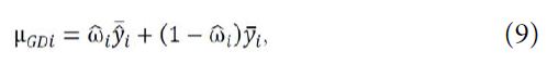
‘s and ![]() ‘s are combined for the estimation of the treatment mean μ. Consider the following weighted-mean estimator,
‘s are combined for the estimation of the treatment mean μ. Consider the following weighted-mean estimator,
![]()
where ![]() It should be noted that
It should be noted that ![]() is the minimum variance unbiased estimator among all weighted-mean estimators when the weight is given by
is the minimum variance unbiased estimator among all weighted-mean estimators when the weight is given by
![]()
if β1, ![]() and
and ![]() are known. In practice,
are known. In practice, ![]() and
and ![]() are usually unknown and ω is commonly estimated by
are usually unknown and ω is commonly estimated by
![]()
where S12 and ![]() are the sample variances of
are the sample variances of ![]() ’s and yj’s, respectively. The corresponding estimator of μ, which is denoted by
’s and yj’s, respectively. The corresponding estimator of μ, which is denoted by
![]()
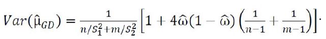
Is referred to as the Graybill-Deal (GD) estimator of μ. The GD estimator is also known the weighted mean in metrology. An approximate unbiased estimator of the variance of the GD estimator, which has bias of order O(n−2 + m−2) is given as
For the comparison of the two treatments, the following hypotheses are considered
![]()
Let ![]() be the predicted value
be the predicted value ![]() , which is used as the
, which is used as the
prediction of y for the jth subject under the ![]() treatment in phase 2. From (7), the Graybill-Deal estimator of
treatment in phase 2. From (7), the Graybill-Deal estimator of ![]() is given as
is given as
where 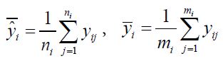 and
and 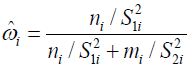 with
with ![]() and
and ![]() being the sample variances of
being the sample variances of 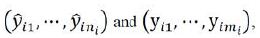 respectively. For hypotheses (8), consider the following test statistic,
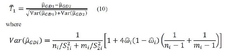
is an estimator of 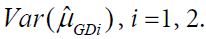 Using arguments similar to those in section 2.1, it can be verified that
 ![]() has a limiting standard normal distribution under the null hypothesis H0 if
has a limiting standard normal distribution under the null hypothesis H0 if
![]()
Consequently, an approximate 100(1-α)% confidence interval of μ1 − μ2 is given as
![]()
where ![]() Therefore, hypothesis H0 is rejected if the confidence interval (9) does not contain 0. Thus, under the local alternative hypothesis that
Therefore, hypothesis H0 is rejected if the confidence interval (9) does not contain 0. Thus, under the local alternative hypothesis that ![]() , the required sample size to achieve a 1−β power satisfies
, the required sample size to achieve a 1−β power satisfies
![]()
Let ![]() Then, denoted by NT the total sample size for two treatment groups is (1+ρ)(1+γ)n1 with n1 given as
Then, denoted by NT the total sample size for two treatment groups is (1+ρ)(1+γ)n1 with n1 given as
![]()
For the case of testing for superiority, consider the following local alternative hypothesis that
![]()
The required sample size to achieve 1−β power satisfies
![]()
Using the notations in the above paragraph, the total sample size for two treatment groups is (1+ρ)(1+γ)n1 with n1 given as
![]()
where  For the case of testing for equivalence with a significance level α, consider the local alternative hypothesis that
 ![]() The required sample size to achieve 1−β power satisfies
The required sample size to achieve 1−β power satisfies
![]()
Thus, the total sample size for two treatment groups is (1+ρ)(1+γ) n1 with n1 given
Note that following similar idea as described above, statistical tests and formulas for sample size calculation for testing hypotheses of equality, non-inferiority, superiority, and equivalence for binary response and time-to-event endpoints can be obtained.
Analysis of Seamless Adaptive Design with Different Target Patient Population
In clinical research, it is often of interest to generalize clinical results obtained from a given target patient population (or a medical center) to a similar but different patient population (or another medical center). Denote the original target patient population by (μ0, σ0), where μ0 and σ0 are the population mean and population standard deviation, respectively. Similarly, denote the similar but different patient population by μ1, σ1. Since the two populations are similar but different, it is reasonable to assume that μ1=μ0 + ε and σ1 =Cσ0 (C > 0), where ε is referred to as the shift in location parameter (population mean) and C is the inflation factor of the scale parameter (population standard deviation). Thus, the (treatment) effect size adjusted for standard deviation of population (μ1, σ1) can be expressed as follows:
![]()
where ![]() and E0 and E1 are the effect size (of clinically meaningful importance) of the original target patient population and the similar but different patient population, respectively. Δ is referred to as a sensitivity index measuring the change in effect size between patient populations [6].
and E0 and E1 are the effect size (of clinically meaningful importance) of the original target patient population and the similar but different patient population, respectively. Δ is referred to as a sensitivity index measuring the change in effect size between patient populations [6].
As it can be seen from (1), if ε = 0 and C = 1, E0 = em>E1. That is, the effect sizes of the two populations are identical. In this case, we claim that the results observed from the original target patient population (e.g., adults) can be generalized to the similar but different patient population (e.g., pediatrics or elderly). Applying the concept of bioequivalence assessment, we can claim that the effect sizes of the two patient populations are equivalent if the confidence interval of |Δ| is within (80%, 120%) of E0. It should be noted that there is a masking effect between the location shift (ε) and scale change (C). In other words, shift in location parameter could be offset by the inflation or deflation of variability. As a result, the sensitivity index may remain unchanged while the target patient population has been shifted.
As indicated by [7], in many clinical trials, the effect sizes of the two populations could be linked by baseline demographics or patient characteristics if there is a relationship between the effect sizes and the baseline demographics and/or patient characteristics (e.g., a covariate vector). In practice, however, such covariates may not exist or exist but not observable. In this case, the sensitivity index may be assessed by simply replacing ε and C with their corresponding estimates [7]. Intuitively, ε and C can be estimated by
![]()
where ![]() are some estimates of (μ0 σ0) and (μ1 σ1), respectively. Thus, the sensitivity index can be estimated by
are some estimates of (μ0 σ0) and (μ1 σ1), respectively. Thus, the sensitivity index can be estimated by
![]()
In practice, the shift in location parameter (ε) and/or the change in scale parameter (C) could be random. Chang [8] studied possible shift in target patient population. If both ε and C are fixed, the sensitivity index can be assessed based on the sample means and sample variances obtained from the two populations. In real world problems, however, ε and C could be either fixed or random variables. In other words, there are three possible scenarios: (1) the case where ε is random and C is fixed, (2) the case where ε is fixed and C is random, and (3) the case where both ε and C are random.
Analysis of k-D seamless adaptive design
When there are differences in study objective, endpoint, and/or target patient population in seamless adaptive designs, some primary assumption and/or statistical considerations are necessarily applied for deriving valid statistical methods for data analysis collected from a given seamless adaptive design. These assumptions and/or considerations are described below.
Primary Assumption and/or Considerations
The “0-D Design” (SSS Design). As indicated in Table 2, SS Design is a two-stage seamless adaptive design with the same study objective and same study endpoint at different stages, which is similar to typical group sequential design with a planned interim analysis. Thus, standard statistical methods such as MIP (method of individual p-values), MSP (method of sum of p-values), and MPP (method of product of p-values) for group sequential design can be directly applied [1,9]. It should be noted that if additional adaptations such as change in primary study endpoint or hypotheses after the review of interim data, the standard methods have to be modified for the control of the overall type I error rate.
The “1-D Design” (DSS, SDS, or SSD Design). Since a “1-D design” could be an SD design or a DS design. Statistical analyses for an SD design and a DS design are different. To have a valid statistical analysis, some assumptions are necessary. For example, for an SD design (i.e., study objectives at different stages are the same but the study endpoints are different at different stages), it is assumed that study endpoint (e.g., a biomarker, a surrogate endpoint, or a clinical endpoint with a short duration) at the first stage is predictive of the study endpoint (i.e., regular clinical endpoint) at the second stage [10]. On the other hand, for a DS design (i.e., study objectives at different stages are different but the study endpoints at different stages are the same), we have to consider testing two sets of hypotheses at different stages [3].
The “2-D Design” (DDS, DSD, or SDD Design). For the “2-D” design (i.e., both study objectives and study endpoints at different stages are different), the following primary assumption and consideration are necessarily made for obtaining a valid statistical test using different endpoints for achieving study objectives at different stages: (i) study endpoint at the first stage is predictive of the study endpoint at the second stage, and (ii) considering testing two sets of hypotheses at different stages.
Chow and Lin (2015) illustrated statistical analysis for a DD design using an example concerning a clinical trial for evaluation of safety, tolerability and efficacy of a test treatment for patients with hepatitis C virus (HCV) infection. In the HCV study, a two-stage seamless adaptive design is considered. The trial design was to combine two independent studies (one phase 2b study for treatment selection and one phase 3 study for efficacy confirmation) into a single study. Thus, study objectives at different stages are similar but different. For the study endpoint, the well-established clinical endpoint is the sustained virologic response (SVR) at week 72 (i.e., 48 weeks of treatment plus 24 weeks of follow-up). Since the PI or sponsor is interested in making early decision for treatment selection at Stage 1. The clinical endpoint of early virologic response (EVR) at week 12 is considered as a surrogate endpoint for treatment selection at Stage 1. Thus, the study endpoints at different stages are different. Statistical test was ten derived based on the primary assumption and consideration for addressing the study objectives at different stages [3].
The “3-D Design” (DDD Design). For the “3-D” design (i.e., study objectives, study endpoints, and target patient populations at different stages are different), the following primary assumption and considerations are necessarily made for obtaining a valid statistical test using different endpoints for achieving study objectives at different stages: (i) study endpoint at the first stage is predictive of the study endpoint at the second stage, (ii) considering testing two sets of hypotheses at different stages, and (iii) the assessment of sensitivity index indicates that there is no significant shift in target patient population from stage to stage.
Examples
Hepatitis C Virus (HCV) Study
A pharmaceutical company was interested in conducting a clinical trial for evaluation of safety, tolerability and efficacy of a test treatment for patients with hepatitis C virus infection. For this purpose, after consulting with regulatory reviewers, it was decided that a two-stage seamless adaptive design would be used for the intended study. The proposed trial design was to combine two independent studies (one phase 2b is study for treatment selection and one phase 3 study for efficacy confirmation) into a single study. Thus, the study consists of two stages: treatment selection (Stage 1) and efficacy confirmation (Stage 2). The study objective at the first stage was for treatment selection, while the study objective at Stage 2 was to establish the non-inferiority of the treatment selected from the first stage as compared to a treatment of standard of care (SOC). Thus, the proposed trial design is a typical “2-D” design, i.e., a two-stage adaptive design with different study objectives at different stages with the same target patient population.
Figure 2 shows the timeline of the “2-D” HCV study. For genotype 1 HCV patients, the treatment duration is usually 48 weeks of treatment followed by a 24-week follow-up. The clinical endpoint is the sustained virologic response (SVR) at week 72. The SVR is defined as an undetectable HCV RNA level (< 10 IU/mL) at week 72. Thus, it will take a long time to observe a response. The pharmaceutical company was interested in considering the same clinical endpoint with a much shorter duration to make early decision for treatment selection of the four active treatments under study at Stage 1. As a result, the clinical endpoint of early virologic response (EVR) at week 12 is considered as a surrogate endpoint for treatment selection at Stage 1. The resultant “2-D” seamless adaptive design is briefly outline below (see also Chow and Lin, 2015) [3]:
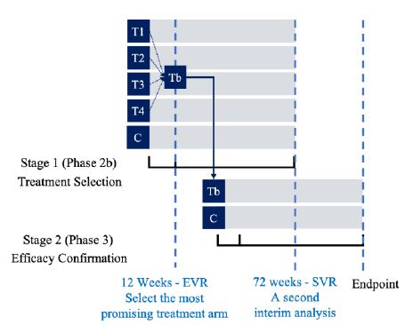
Figure 2: Timeline of the “2-D” HCV study
Stage 1. At this stage, the design begins with five arms (4 active treatment arms and one control arm). Qualified subjects were randomly assigned to receive one of the five treatment arms at a 1:1:1:1:1 ratio. After all Stage 1 subjects have completed Week 12 of the study, an interim analysis was performed based on EVR at week 12 for treatment selection. Treatment selection was made under the assumption that the 12-week EVR is predictive of 72-week SVR. Under this assumption, the most promising treatment arm was selected using precision analysis under some pre-specified selection criteria that the treatment arm with highest confidence level for achieving statistical significance (i.e., the observed difference as compared to the control is not by chance alone) was selected. Stage 1 subjects who have not yet completed the study protocol continued with their assigned therapies for the remainder of the planned 48 weeks, with final follow-up at Week 72. The selected treatment arm was then proceeded to Stage 2.
Stage 2. At Stage 2, the selected treatment arm from Stage 1 was test for non-inferiority against the control (SOC). A separate cohort of subjects was randomized to receive either the selected treatment from Stage 1 or the control (SOC) at a 1:1 ratio. A second interim analysis was performed when all Stage 2 subjects have completed Week 12 and 50% of the subjects (Stage 1 and Stage 2 combined) have completed 48 weeks of treatment and follow-up of 24 weeks. The purpose of this interim analysis was two-fold. First, it was to validate the assumption that EVR at week 12 is predictive of SVR at week 72. Second, it was to perform sample size re-estimation to determine whether the trial will achieve study objective (establishing non-inferiority) with the desired power if the observed treatment preserves till the end of the study. Statistical tests as described in the previous section was presented to test non-inferiority hypotheses at interim analyses and at end of stage analyses. For the two planned interim analyses, the incidence of EVR at week 12 as well as safety data, were reviewed by an independent data safety monitoring committee (iDMC). The commonly used O’Brien-Fleming type of conservative boundaries was applied for controlling the overall Type I error rate at 5%. Adaptations such as stopping the trial early, discontinuing selected treatment arms, and re-estimating the sample size based on the pre-specified criteria were applied as recommended by the iDMC.
Non-Alcoholic SteatoHepatitis (NASH) Clinical Trials
For development of drug products for treating patients with NASH, after having consulted with regulatory agency, it is suggested the following clinical trials utilizing seamless adaptive designs may be useful to shorten and speed up the process of NASH drug product development: (i) proof-of-concept/dose ranging adaptive trial design,(ii) phase 3/4 adaptive trial design, and (iii) phase 2/3/4 adaptive design [11].
Table 4 illustrates the objectives, endpoints and target patient populations in NASH clinical trials. For illustration purpose, consider a single seamless phase 2/3/4 adaptive trial design allows adaptations, continuous exposure, and long-term follow-up (Figure 3). Endpoints at interim analysis are (i) reduction of at least 2 points in NAS, (ii) resolution of NASH by histology without worsening of fibrosis, and/or (iii) improvement in fibrosis without worsening of NASH [12-15]. One (the most promising dose) or two doses may continue to the next phase. A post-marketing phase 4 with demonstration of improvement in clinical outcomes will lead to final marketing authorization.
Because only one trial would lead to approval, a very small overall alpha (i.e., <0.001) is recommended to ensure proper control of a type I error.
Although the above seamless phase 2/3/4 appears to be reasonable, regulatory agency such as FDA [16-18] emphasizes that the designs must be supported by a sound rationale and scientific justifiable for integrity, quality and validity. Protocol should address the following typical issues:
(i) Provide detailed information regarding how the overall type I error rate is controlled or preserved;
(ii) Provide a detailed strategy or plan for preventing possible operational biases that may incur before and after the adaptations are applied;
(iii) Provide justification regarding the validity of statistical methods used for a combined analysis;
(iv) Provide justification for the chosen alpha spending function (e.g., O’Brien-Fleming) for stopping boundaries;
(v) Provide justification regarding criteria used for critical decision-making at interims;
(vi) Establish an independent data safety monitoring committee (IDMC) and provide IDMC charter;
(vii) Provide justification for power analysis for sample size calculation and sample size allocation especially where the study objectives, endpoints, and populations are different at different stages;
(viii) Provide justification if sample size re-estimation is performed in a blinded or unblended fashion in the seamless adaptive trial design.
Table 4: Objectives, Endpoints and Target Patient Populations in NASH Clinical Trials.
|
Objective |
Primary Endpoint |
Target Patient Population |
| Trials to support a marketing application | Composite endpoint: complete resolution of steatohepatitis and no worsening of fibrosis –
Composite endpoint: At least one point improvement in fibrosis with no worsening of steatohepatitis (no increase in steatosis, ballooning or inflammation) |
Biopsy confirmed NASH patients with moderate/advanced fibrosis (F2/F3) |
| Clinical outcome underway by the time of submission:
Histopathologic progression to cirrhosis MELD score change by >2 points or MELD increase to >15 in population enrolled with ≤ 13 •Death •Transplant •Decompensation events –Hepatic encephalopathy – West Haven ≥ grade 2 –Variceal bleeding – requiring hospitalization –Ascites – requiring intervention –Spontaneous bacteria peritonitis
|
||
| Dose ranging/Phase 2 | Improvement in activity (NAS)/ballooning/inflammation without worsening of fibrosis can be acceptable
Include a subpopulation with moderate/advanced fibrosis (F2/F3) to inform PhIII |
Biopsy proven NASH (NAS ≥ 4)
–Include patients with NASH and liver fibrosis with any stage of fibrosis Include patients with NASH and ≥ Fibrosis stage 2 to inform PhIII |
| Early phase trials/Proof of concept | Endpoints should be based on mechanism of drug
Consider using improvement in NAS (ballooning & inflammation) and/or fibrosis Reduction in liver fat with a sustained improvement in transaminases
|
Ideal to use patients with biopsy proven NASH, but acceptable to use patients at high risk for NASH (fatty liver + type 2 diabetes, the metabolic syndrome and high transaminases are acceptable |
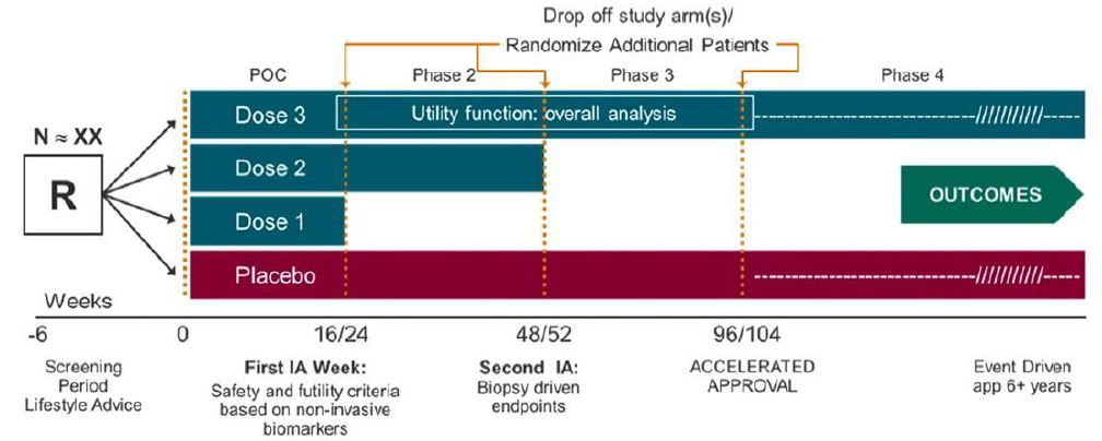
Figure 3: Phase 2/3/4 Seamless Adaptive Design.
The NASH clinical trial design is a typical “3-D” design. The analysis of a “3-D” seamless adaptive trial design requires (i) a primary assumption that the study endpoint at the first stage is predictive of the clinical endpoint at the second stage to account for different study endpoints at different stages, (ii) a consideration of testing two sets of hypotheses to account for different study objectives at different stages, and (iii) a sensitivity analysis to account for a possible shift in target patient population from stage to stage.
Conclusion
In this article, depending upon whether the study objectives, study endpoints, and target patient populations at different stages are different, two-stage seamless adaptive designs are classified into eight different categories, namely, “0-D” design, “1-D” design, “2-D” design, and “3-D” design. For a given type of two-stage seamless adaptive trial design, the following proposal is made for a valid statistical analysis. First, a primary assumption that the study endpoint at the first stage is predictive of the study endpoint at the second stage is made to account for different study endpoints at different stages. Second, a consideration of testing two sets of hypotheses is suggested to account for different study objectives at different stages. Third, it is suggested that an assessment of a sensitivity index should be performed for possible shift in target patient population from stage to stage. Two examples concerning a hepatitis C virus (HCV) infection clinical study (a typical “2-D” design) and a non-alcoholic steatohepatitis (NASH) clinical trial (a typical “3-D” design) are presented to illustrate the proposed methods. From regulatory perspectives, the innovative seamless adaptive trial designs discussed in this article cannot only offer great flexibility of identifying any signal, trend, or optimal benefit of the test treatment under investigation, but also improve the relative efficiency (e.g., shorten the development process). However, these can only be achieved at the risk of controlling the overall type I error rate and/or the validity and integrity of the intended clinical trials. From statistical perspectives, on the other hand, for most innovative seamless adaptive trial designs, statistical methods are not fully established. Although clinical simulation may provide a solution, it is not “the” solution because the model used for simulation is difficult, if not impossible, to verify. A wrong model could lead to biased conclusion and hence may be misleading. Never misuse or abuse the use of complex seamless adaptive trial design in clinical research and development. From clinical perspectives, it is suggested that an “investigator’s wish list” approach should be considered when applying complex innovative design in clinical research. In other words, clinician should always be in the driver seat and biostatistician should development statistical tests with optimal statistical properties to accommodate the investigator’s wish list without undreaming the validity and integrity of the intended trial.
References
- Chow SC, Chang M (2011) Adaptive Design Methods in Clinical Trials. 2nd edition, Chapman and Hall/CRC Press, Taylor & Francis, New York, New York.
- EMA (2014) Pilot project on adaptive licensing. European Medicines Agency, London, UK.
- Chow SC, Lin M (2015) Analysis of two-stage adaptive seamless trial design. Pharmaceutica Analytica Acta 6.
- Chow SC, Corey R (2011) Benefits, Challenges and obstacles of adaptive designs in clinical trials. The Orphanet Journal of Rare Diseases 6. [crossref]
- Chow SC (2020) Innovative Methods for Rare Disease Drug Chapman and Hall/CRC Press, Taylor & Francis, New York.
- Shao J, Chow SC (2002) Reproducibility probability in clinical trials. Statistics in Medicine, 21: 1727-1742.
- Chow SC, Shao J (2005) Inference for clinical trials with some protocol amendments. Journal of Biopharmaceutical Statistics 15: 659-666. [crossref]
- Lu Y, Kong YY, Chow SC (2017) Analysis of sensitivity index for assessing generalizability in clinical research. Jacobs Journal of Biostatistics 2.
- Chang M (2007) Adaptive design method based on sum of p-values. Statistics in Medicine 26: 2772-2784. [crossref]
- Chow SC, Lu Q, Tse SK (2007) Statistical analysis for two-stage adaptive design with different study endpoints. Journal of Biopharmaceutical Statistics 17: 1163-1176. [crossref]
- Filozof C, Chow SC, Dimick-Santos L, Chen YF, Williams RN, et al.. (2017) Clinical endpoints and adaptive clinical trials in precirrhotic nonalcohotic steatohepatitis: facilitating development approaches for an emerging epidemic. Hepatology Communications 1 ; 577-585. [crossref]
- Argo CK, Northup PG, Al-Osaimi AM, Caldwell SH (2009) Systematic review of risk factors for fibrosis progression in non-alcoholic steatohepatitis. J Hepatol 51: 371-379. [crossref]
- Brunt EM, Kleiner DE, Wilson LA, Belt P, Neuschwander-Tetri BA (2011) NASH Clinical Research Network (CRN) Nonalcoholic fatty liver disease (NAFLD) activity score and the histopathologic diagnosis in NAFLD: distinct clinicopathologic meanings. Hepatology 53: 810-820. [crossref]
- Ekstedt M, Franzen LE, Mathiesen UL, Thorelius L, Holmqvist M, et al. (2006) Long-term follow-up of patients with NAFLD and elevated liver enzymes. Hepatology 44: 865-873. [crossref]
- Angulo P, Kleiner DE, Dam-Larsen S, Adams LA, Bjornsson ES, et al. (2015) Liver fibrosis, but no other histologic features, is associated with long-term outcomes of patients with nonalcoholic fatty liver disease. Gastroenterology 149: 389-39. [crossref]
- FDA (2014) Guidance for Industry – Expedited Programs for Serious Conditions – Drugs and Biologics. The United States Food and Drug Administration, Silver Spring, Maryland.
- FDA (2018) Guidance for Industry – Noncirrhotic Nonalcoholic Steatohepatitis With Liver Fibrosis: Developing Drugs for Treatment. The United States Food and Drug Administration, Silver Spring, Maryland.
- FDA (2019) Guidance for Industry – Adaptive Designs for Clinical Trials of Drugs and Biologics. The United States Food and Drug Administration, Silver Spring, Maryland, November 2019.