Abstract
The study reported here on ‘what does it take to become a police officer’ represents one of several explorations of the ‘world of the adult’ from the point of view of a middle school student. The objective of these studies is to explore the nature of how students see the world of adults, doing so by providing the student with a templated research tool (www.BimiLeap.com). With this tool, and with the embedded coaching provided by the access to artificial intelligence (Idea Coach), the student can explore a topic, select aspects of the topic, and perform a real-world experiment, in the same way as a professional researcher does. The outcome shows how the student thinks about a topic, and the response to the student’s thinking by actual respondents, an outcome which at once provides knowledge about the topic and knowledge about the mind of the researcher.
Introduction
A great deal of the research involving the way young people think comes from the world of developmental psychology, with its emphasis on the nature of how the young person approaches a problem, conceptualizes the problem, and then proceeds to solve the problem. The literature of developmental psychology is vast, much of it in the hands of professional psychologists who study the topic in the rarified atmosphere of observational science [1,2]. The science, the knowledge emerging, may be idiographic, viz., detailed knowledge of an individual, or nomothetic, viz., detailed knowledge of general patterns of groups. Of interest here is how children think about future careers, specifically a career in the police force [3-6].While scientists and clinicians build up their world of understanding, there are practical issues and applications as well, best expressed by issues encountered in school and in everyday life. How does a student learn? What are the types of questions that a student asks about a topic? One example is how do students formulate questions about a topic to learn about the topic. What can we learn from those questions? And can we create a system which allows us to explore the mind of the student towards the world of the everyday?
A continuing topic in science concerns what is appropriate for science to investigate, who should do the investigation, how should the investigation be done, what should be the appropriate report, and finally what is the ultimate value of the research? For the efforts involving student researchers, often young ones who have not even graduated high school or middle school, the question revolves around the nature of the contribution that they can make. The world of academic science is replete with degreed professionals, publishing papers on topics to, in colloquial terms, ‘answer a call from the literature’ or plug a hole in the gaps of our knowledge.’ There is a sense that science is evolving to a closed world, permission to join that world granted only by degree, and only by the receipt of money to do one’s scientific research. There is no room for others. Sadly, then, this attitude, if correct, may end up limiting our knowledge about the psychology of people, especially young people, as these people focus on real-world issues. The young people may end up as subjects for the study, the study involving an external researcher trying to figure out the ideas of the young person. Why not let the young person do the research, choosing the topic, and executing the study in a way which ensures the maximum opportunity of success.
The Worldview of Mind Genomics
Mind Genomics is an emerging science, focusing on the analysis of how we make decisions about the world of the everyday [7,8]. Of relevance to the understanding of the mind of young people are at least two studies dealing done with Mind Genomics, one on hospitals [9], the other on the marketing of museums to young people [10]. Mind Genomics has emerged slowly during the past forty years, with roots and history traceable to at least three worlds of inquiry:
The first of the worlds is experimental psychology, and specifically the world of psychophysics, the study of the relation between test stimuli and the perception of these test stimuli. Psychophysics is often thought to be the earliest field of experimental psychology, with a focus on measuring the perceived intensity of test stimuli, such as the sweetness of a cola sweetened beverage. The traditional objective of psychophysics is to measure the subjective intensity of external stimuli, such as the loudness of sounds, and so forth. Mind Genomics moves the measurement inwards, to measure the magnitude of private sensory or cognitive experience. The goal, however, remains measurement.
The second world is statistics, and more specifically the role of experimental design. Mind Genomics ‘works’ by presenting vignettes (combinations of elements, viz., messages) to the respondent with the instruction to read the vignette, and rate the entire vignette as a single entity. The rationale is that in the world of the everyday the person is confronted with mixtures of elements, from which the respondent must make a decision. The person is almost never presented with a series of single elements, one at a time, and instructed to make a decision. That ‘one at a time’ strategy simply does not represent the world in which people naturally make decisions. The issue is to create the appropriate set of combinations or vignettes, allowing the researcher to uncover how each element drives the response. In other words, the respondent evaluates systematically constructed mixtures, allowing the researcher to estimate the contribution of each component of the mixture. It is statistics, specifically experimental design, which prescribes the specific combinations to create and to test [11].
The third world is consumer research, more specifically the evaluation of real-world concepts, viz., meaningful combinations of elements. Consumer research deals with topics that are meaningful and real in the everyday world, in contrast to experimental psychology and psychophysics which deal with artificially contrived situations having little or no cognitive value. A consumer researcher works with test stimuli which have meaning in the outside world. Just the word ‘consumer’ in the name ‘consumer research’ is a clue that the topics must have relevance to the real world of people, not to artificially contrived situations set up to support or disprove a hypothesis.
Templating the Mind Genomics Studies to Democratize the ‘Project of Science’
During the forty-year history of Mind Genomics, as it evolved from business-oriented studies of what to say about products into a more general understanding of how people think about topics, it became increasingly obvious that the process of creating vignettes to test was a barrier. In today’s language, the need to think about topics, to create test stimuli, and to execute and analyze experiments became ‘friction points.’ Even students, accustomed to research projects, reported that they had difficulty developing combinations of ideas to test, although few students ever reported difficulties with the ensuing statistical analysis of the data once the study was designed and executed.
During that forty year period it was becoming increasingly obvious that the process of Mind Genomics had to be streamlined, both to help the researcher develop the test stimuli / run the experiment, but also, and more profoundly, help the researcher to think in a new way. It was at this point that the effort moved towards templates, and to automating the process, an effort evolving to the use of artificial intelligence as a coach to help create the questions and the answers [12].
This paper presents the templated approach, applying it to a specific study developed entirely by the senior author, Cledwin Mendoza, himself a middle school student. It is important to keep the nature of the lead researcher in mind because the paper will reveal a way by which the world can be studied from the ‘inside out’, viz., from the mind of young people who are just entering the world, rather than being studied from the ‘outside in’, by professionals who are trying to understand what the young person is thinking, but doing it through a blunt instrument and a blurry lens.
The steps presented below are implemented in an easy-to-use computer program, www.BimiLeap.com. The program is free to use, with the only charges being the minor cost of acquiring information from the artificial intelligence source (Open AI), and the relatively minor cost of actually running a study with real people.
The Steps in the Process
Step 1: Describe the Topic in a Word or Two (Figure 1)
This step may seem simple, but it forces the researcher to focus on the issue. This first step begins the development of critical thinking about the topic, as the research is forced to distinguish between the topic in general (to be written in the proper space in Figure 1), and the actual question about the topic (to be written in Figure 2, where the researcher is requested to expand on the topic.
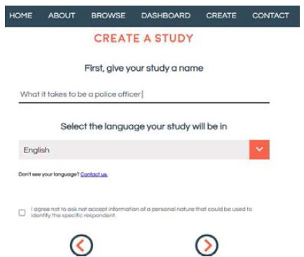
Figure 1: The front page, requesting the researcher to name the study
Step 2: Come Up with Four Questions Pertaining to the Topic (Figure 2)
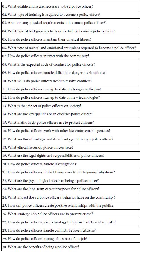
It is at this point that many researchers and students ‘freeze.’ It is one thing to name a topic, but quite another to think deeply about a topic, coming up with a set of four questions which are coherent, and which tell a story. The Mind Genomics process has been immeasurably aided by the emergence of artificial intelligence provided by Open AI, Inc., and embedded in Idea Coach. Panel B shows the screen shot with the ‘box’ in which the researcher can describe the topic, either in sketchy terms or in detail, as desired. Idea Coach then returns with a set of up to 30 recommended questions that can be used (Panel 2C). The researcher may select some of the questions, and repeat the request, using either the same description of the topic, or a revised description. Idea Coach will return with another set of 30 questions, some of which may be repeats from the first set of 30. Panel D lists the final set of four questions. The Idea Coach in Step 2 serves both as a tool to facilitate the research and to engage the researcher to think more deeply about the topic. Table 1 presents a set of 30 questions emerging from the request. The entire set-up process takes about 10 minutes or less once the researcher becomes familiar with the process of using Idea Coach. It is important to emphasize that Step 2 enables the researcher to learn about the topic in a way that ends up being deep and granular.
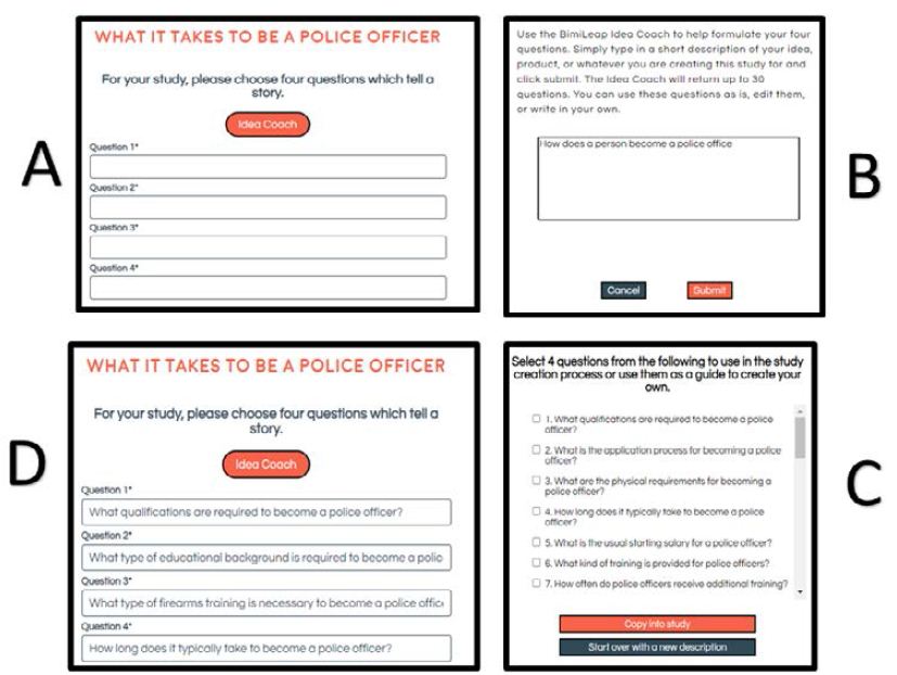
Figure 2: The request for the four questions (Panel A), the Idea Coach (Panel B), some of the questions returned (Panel C), and the four questions finally selected (Panel D).
Table 1: The 30 questions emerging from using Idea Coach
Step 3: Create Four Answers for Each of the Four Questions
Answering questions ends up being easier than posing questions. Once the researcher has chosen the four questions, the researcher can either answer the questions directly, or once again use artificial intelligence embedded in Idea Coach to create the answers. Once again the researcher can use Idea Coach a number of times for each question to identify appropriate answers. Each ‘query’ to Idea Coach returns with 10-15 answers. Depending upon the nature of the topic the answers can be the same or different. There is no direct control. Figure 3 shows the process as the researcher would see it. Table 2 shows three different runs of the same question, creating 45 answers, many of which are the same from run to run.
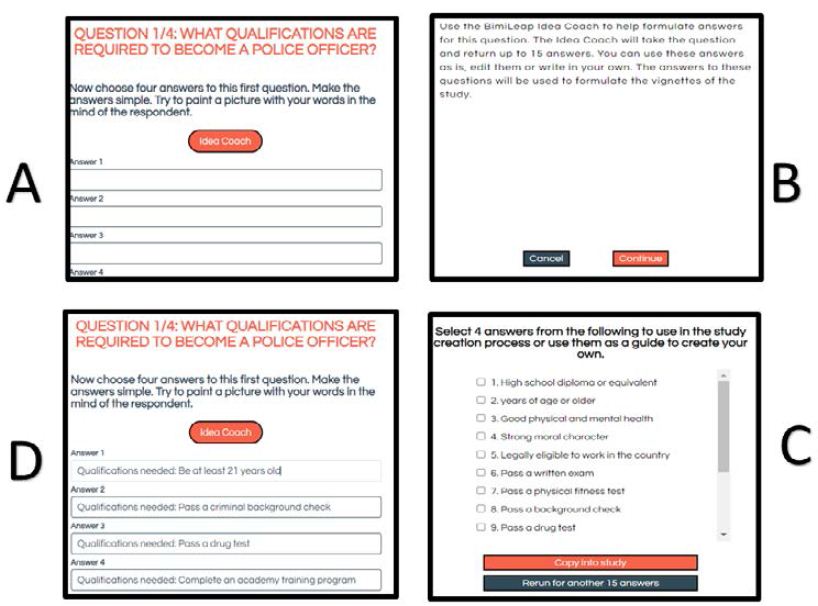
Figure 3: The instruction to create four answers for Questions
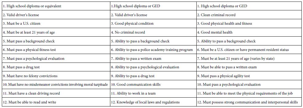
Table 2: Three sets of 12 suggested answers to question 1 provided by Idea Coach. The question is ‘What qualifications are required to become a police officer?”
Step 4: Create Vignettes Comprising 2-4 Elements
Mind Genomics works by presenting vignettes to respondents, these vignettes comprising a limited number of elements. The vignettes attempt to describe a ‘scenario’ with sufficient information to allow the respondent to assign a rating. The vignettes are created according to an underlying experimental design. The design for the specific set of four questions and four answers to each question requires 24 combinations. These combinations can be modified by a permutation scheme, one which maintains the underlying mathematical structural, but ensures that each set of 24 combinations differs substantially from every other set of 24 combinations. Each of the 16 elements in the 24 combinations appears exactly five times, and is absent exactly 19 times. Each vignette comprises at most one element or answer from a question, never two answers from the same question, and in five of the 24 vignettes the element or answer from the question is entirely absent.
Figure 4 shows an example of the vignette (and the rating question and scale) as it would be presented to the respondent. The respondent does know that the vignettes are created by an underlying design, and indeed it would be impossible for the respondent to detect such a design in the short time that the respondent participants.
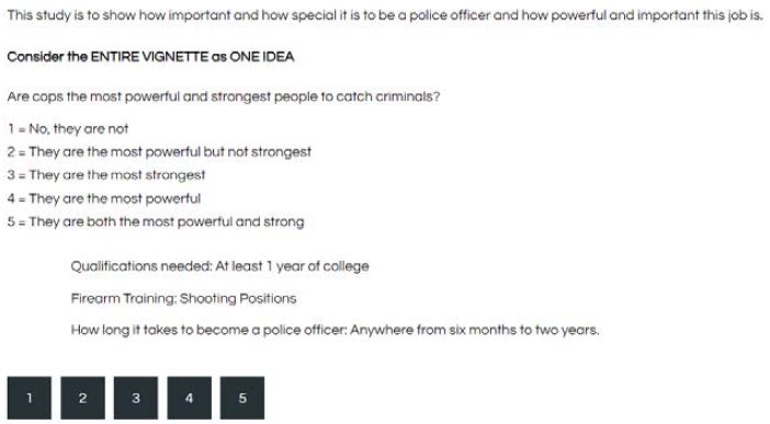
Figure 4: Example of the vignette as the respondent sees it. The figure shows the rating question, the vignette
Step 5: Complete the Study set-up
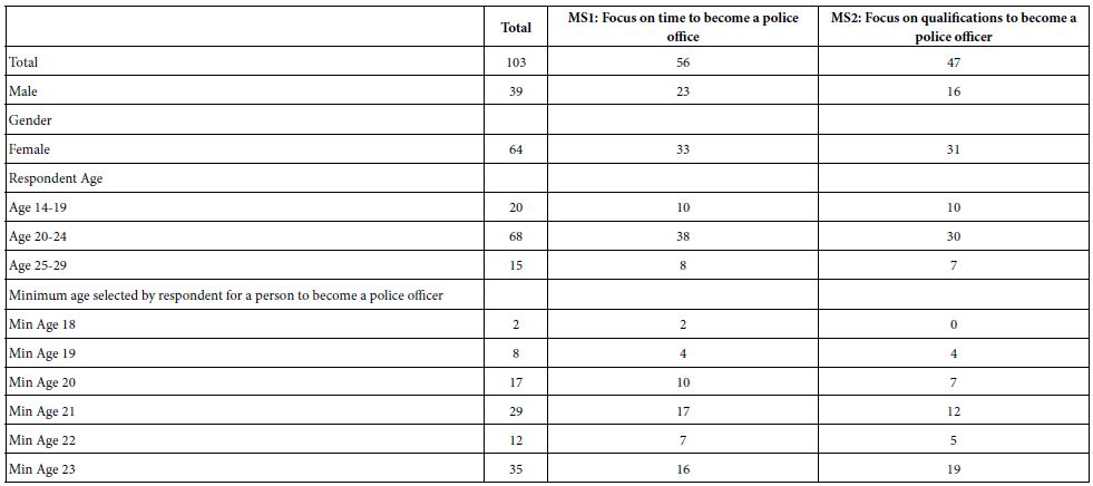
The set-up includes the creation of a set of self-profiling classification questions, two fixed (gender, age), and up to eight more left to the researcher. The rest of the study includes the rating question, the rating scale, an open end-question if desired, and a small paragraph to record the underlying objective of the study. Table 3 shows the relevant information for the study, including the number and gender of the respondents. This information is returned in the Excel report which summarizes the study and its data. Once the study is finalized, the researcher launches, choosing either paid respondents, or respondents that will be furnished by the researcher (Figure 5). Although it is always more attractive to work with one’s own associates/friends/students as respondents, experience suggests that study with 100 respondents may take an hour or two to complete with ‘paid respondents’, and a week or two or even longer, sometimes never, to complete with one’s ‘unpaid respondents.’
Table 3: Relevant study information for the study returned in the Excel report
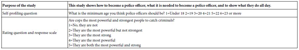
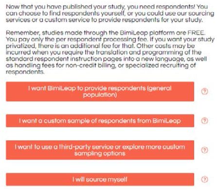
Figure 5: Options to source respondents from (www.BimiLeap.com, the Mind Genomics website
Step 6: Sourcing Respondents
During the past decade the volume of surveys has increased dramatically, as the desire for consumer feedback has exploded. Consequently, the so-called ‘response-rate’ has dropped down. Whereas decades ago the participation in a survey was deemed interesting, today the same participation is considered an intrusion. It is difficult, almost impossible at times, to secure respondents for free, unless one is dealing with a captive audience. The best way to get willing respondents is to pay them, or to work with an on-line panel provider who incentivizes the respondent to participate in these surveys, e.g., through points which can be redeemed for something, even occasionally for money. Whether these respondents are somehow biased or not representative of the ‘real world’ was once an issue for the purist researcher, but today’s oversampled, survey-weary individuals make that issue of ‘real world’ virtually irrelevant.
The BimiLeap program has within it a variety of options to source respondents, as Figure 5 shows. The efforts to source respondents do cost some money, but minimal amounts in the world of today. For those who want to source their own respondent there is that option. For those who want a professional group to provide a group of specified types of individuals there is that option as well.
Step 7: Acquiring the Data and Storing the Data in an Analysis-ready Database
The respondents were provided by Luc.id, Inc. BimiLeap contains a set of screens allowing the researcher to specify the respondents. For this study, the respondents were selected to be residents of the United States, and to be between the ages of 16 and 30. The BimiLeap program is set up to forward the request automatically to Luc.id, when the researcher selects BimiLeap as the provider.
The appropriate respondents who fit the criteria selected by the researcher are invited to participate. Those who participate are shown a series of screens, introducing the topic, requesting the respondent to complete the self-profiling questionnaire, and then read and rate each of the 24 vignettes. Recall that each respondent evaluated a unique set of 24 vignettes, as specified by the underlying experimental design [13].
Figure 6 shows an example for three vignettes evaluated by one of the respondents. The left column shows the respondent (cut off for this respondent), the 2nd column shows the text of the vignette, the 3rd column shows the rating, and the 4th column shows the response time.
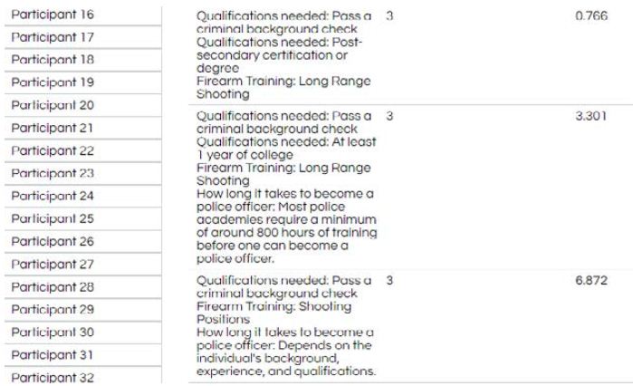
Figure 6: Example of data as captured by the Bimileap program
Step 8: Create Equations Relating the Presence/Absence of Elements to Ratings and to Response Time
The goal of Mind Genomics is to quantify the relation between the presence/absence of the elements and the response. The response in this case is the rating assigned by the respondent on the 5-point scale (or more correctly a transformed value, described below), and well as the response time.
The first action to create the equations is to put the rating into the proper form. The scale by itself has to be transformed so that the numbers are meaningful. The scale as presented is known as a nominal scale. The scale does not have metric meaning. Fortunately, the transformations that can be made are easy to do, as presented below.
For this study we focus on Rating 5. The rating question is: Are cops the most powerful and strongest people to catch criminals? Rating 5 is: They are both the most powerful and strong.
Our interest then is whether the respondent feels that that, based on the vignette, does the respondent rate the vignette ‘5’ or not. When the respondent rates the vignette ‘5’, then we create a new variable, called R5, and give R5 the value ‘100’. When the respondent rates the vignette ‘1, 2, 3 or 4’, then we give R5 the value ‘0’. In this way we end up with a new variable ‘5’ which has a defined, straightforward meaning. Furthermore, a manager presented with an average value of 45 for R5, for example, the manager immediately knows that 45% of the responses were ‘5’, and the remaining 55% of the responses were not ‘5’. Note that in this study only the rating of ‘5’ was transformed to 100, with the remaining four rating points transformed to ‘0’. In other studies, often the ratings of both ‘5’ and ‘4’ are transformed to 100. The reason for the focus on rating ‘5’ is the interest in perceiving the police officer as both powerful and strong. Finally, after the binary transformation has been made, a vanishingly small random number is added to the transformed number, moving it away from purely ‘0’. This action is prophylactic, preventing the respondent from ending up with all ‘0’s,’ or with all ‘1’s,’ respectively, a situation which would cause the regression program to ‘crash.’ The regression program requires some minimal level of variation in the dependent variable.
The second action is to bring in the response time and truncate it to the nearest 100th of a second. There is no transformation needed here.
Once the transformations are made, the database can be easily created. Each respondent generates 24 rows in this database. The columns are defined as follows:
Column 1 Study name
Column 2 Respondent unique identifier
Columns 3-5 Specific information from the self-profiling classification (here gender, age, and appropriate age…)
Column 6-21 Coding for the element. Each column corresponds to an element (A1-D4). For a specific respondent and a specific vignette, the cell has the value ‘1’ when the element appears in the vignette, or the value ‘0’ when the element is absent from the vignette.
Column 22 Order of testing (1-24)
Columns 23-24 Rating, Response Time,
Columns 25-29 Binary Transformed Ratings (R1, R2, R3, R4, R5)
Once the data are transformed, it is straightforward to create the equation relating the presence/absence of the 16 elements to the transformed (binary) variable for R5, and to response time. The approach is known as OLS, ordinary least-squares, with the variables being known as ‘dummy variables,’ because the variables are either ‘0’ (absent) or ‘1’ (present).
The regression equation for R5 (transformed binary rating) is: R5 = k0 + k1(A1) + k2(A2) … k16(D4)
The equation tells us that the binary value R5 is the sum of an additive constant (k0) and the weighted values for the 16 elements. The additive constant is a purely theoretical baseline, showing the expected value of the binary variable R5 when all the 16 elements are absent from the vignette. The reality is that the underlying experimental design ensures that each respondent evaluated vignettes comprising a minimum of two elements and a maximum of four elements, so in no case was a vignette ever shown without elements. Nonetheless, the regression equation estimates that value, as a ‘correction factor’. IN the language of statistics, k0 is known as the ‘intercept’, viz the value of Y when X is 0, or in our case the value of R5 when all the 16 X’s, the 16 elements, are 0. We use the value R5 as a measure of the basic predilection of a person or a group of respondents to select the rating of ‘5’.
The coefficient for an element (viz., k1 – k16) tells us the percentage of respondents who will change their rating to ‘5’ when they evaluate a vignette with the element in the vignette. Thus, for a coefficient of 3 for an element, an additional 3% of the respondent who read a vignette with that particular element changed their rating from ‘1, 2, 3 or 4’ to a rating of ‘5’. Our focus will be on the elements and the subgroups showing high coefficients, typically 6 or higher. Continuing with our train of thought, a coefficient of +6 for an element means that an additional 6% of the responses for a vignette containing this element will shift from a lower range of 1-4 to the higher value of 5.
The regression for RT (response time) is expressed by the same equation, but without an additive constant: RT = k1(A1) + k2(A2) … k16(D4). Response time does not need an additive constant. We assume that in the absence of all elements there is no response at all, so by definition the response time is already 0.
Step 9: Create Mind-sets Using Clustering
People are different. We often pay attention to the large differences among people, feeling that these are worthy of note. Marketers attempt to divide the world into these different basic groups, the groups being relevant to large-scale topics and issues such as political leaning (e.g., progressive vs. conservative), financial issues (e.g., growth seeking vs. capital protection), food preferences (adventurous eaters vs. conservative eaters), and the like. The contribution of Mind Genomics is to find these differences in the world of the everyday. An early discovery of Mind Genomics was that it is a straightforward approach to uncover these group differences within a single dataset using relatively straightforward statistics.
For our data on police, or for that matter, any data of this type, the process to uncover these mind-sets, these groups of different-thinking individuals, uses a combination of regression analysis and cluster analysis. The overall goal is to create an individual-level equation for each respondent, then using the coefficients of the model for each respondent to define a ‘distance’ between each pair of respondents, and finally put the individuals in a small number of groups or clusters (viz., mind-sets) so that the pattern of coefficients is similar within a group or mind-set, but the groups are different from each other. The outcome, however, ends up being a small number of groups which have radically different patterns of coefficients, patterns which presumably lend themselves to easy interpretation.
The clustering used in this study is called k-means cluster [14]. The clustering approach creates an equation for each respondent, relating the dependent variable, R5, to the 16 elements. The estimation of the individual-level model is possible because the 24 vignettes for each respondent are set up to allow OLS regression for that individual, even if there is no other respondent. The measure of distance between the respondents is (1-Pearson R), with the Pearson R (correlation) measuring the degree of linearity between two sets of 16 coefficients (the additive constant not considered). The distance between two perfectly correlated sets of 16 coefficients is 0 (1-1 = 0). The distance between two opposite patterns is (1)-(-1), viz., 2. Once the person-to-person distances are computed, as well as the centroid-to- centroid differences computed, the clustering program can identify the number of clusters, and the appropriate membership of each respondent in one of the non-overlapping, exhaustive clusters. For these data the cluster solution suggested two groups, called MS1 and MS2 (MS short for mind-set).
Results
Table 4 shows the panel composition:
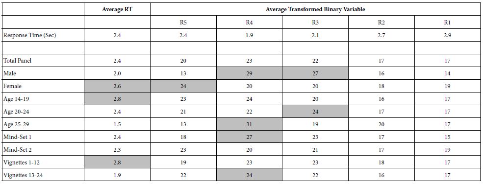
We begin the exploration of the data with the simplest analysis, namely the average response time, and the average transformed ratings, first for total panel, and then for key subgroups. Table 4 shows the averages. The columns correspond to the dependent variable, the first being the average response time across all vignettes evaluated by the key subgroup, and the remaining five being the average transformed ratings, R1-R5. The final analysis looks at the averages for the first 12 vignettes, and then the second 12 vignettes. To allow patterns to emerge, Table 4 presents strong performing elements in shaded cells. These strong performing elements are response times of 2.6 seconds or longer, and average transformed variable of 24 or higher. The pattern is clear for the order of testing, with vignettes 1-12 generating longer response times than vignettes 13-24. Yet, beyond that simple finding, it is hard to state anything about the results. By itself, Table 5 may allow one to generate hypotheses about ‘why’ certain ratings (R5, R2, R1) co-vary with long responses times, whereas other ratings (R4, R3) co-covary with short response times. Table 4, however, does not allow the researcher to exploit the most important feature of the stimuli, viz., that the test stimuli, the elements, are ‘cognitively rich,’ replete with meaning, and interpretable in and of themselves.
Table 4: Panel composition
We now move to the explication of the data after OLS (Ordinary Least Squares) regression. The dependent variable is R5, The rating question is: Are cops the most powerful and strongest people to catch criminals? Rating 5 is: They are both the most powerful and strong. R5 takes on the value ’100’ when the respondent selects ‘5’ as the rating. R5 takes on the value ‘0’ when the respondent selects any other number, ‘1, 2, 3, or 4’.’
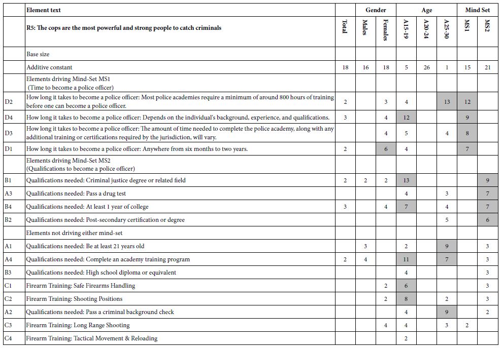
The coefficients for the equation (models) for the studies are shown in Table 5. The columns correspond to the defined groups of respondents or vignettes, the rows correspond to the additive constant, and then to the 16 elements. All coefficients of 1 or lower are removed, so that the cell is empty. Strong performing elements (operationally defined as a coefficient of +6) are shown by shaded cells. The table is sorted by the values for the coefficients emerging from the mind-sets.
Table 5: Average response time and transformed binary variable for total panel and key subgroups
The rationale for not showing very low, 0 or negative coefficients is that these negative coefficients show that the element does not drive R5. We are interested in the elements which drive R5. The rationale for shading the strong performing cells is to allow the patterns to emerge more clearly. Finally, the rationale for sorting the table by the coefficient of the two mind-sets that only then does a strong and meaningful pattern emerge.
Table 6 shows four sets of columns, corresponding to the key groups.
- The additive constant is 18, meaning that about one out of five or six responses is ‘5’. This is a low baseline. As we scan the table, looking at the column for Total, see remarkably few elements. It is as if there are no strong messages. It is important to stop to think about what this means. Is it the case that the researcher simply failed to find the ‘right words’ to drive the strong responses? Or is the reason deeper, that perhaps looking at the Total is not a productive approach, that perhaps there will never be the ‘magic messages’ which generate high coefficients among the total panel. It is important to note that this conundrum, about low coefficients among the total panel, is a lesson for the young researcher that there is no perfect message, and that it might be futile to continue in that path, looking for the ‘better message’. Finally, the disappointing results for the Total Panel do not surprise us. They emerge again and again in these studies and in the outside where the data are used to make product development and marketing decisions. There are no ‘perfect’ and when a high scoring element is achieved for the Total Panel, it is an unexpected anomaly.
- Once again, the additive constants are low, 16 for males, 18 for females. And once again most coefficients are absent. There are few positive coefficients and no operationally defined ‘strong performing elements’ with coefficient of +6 or higher.
- It is when we get to age that we begin to see patterns emerging, patterns which show us different ways of thinking. When we look at these patterns in detail, however, we will see that the patterns emerge from the general magnitudes of the response, and not from profoundly different ways of looking at the work. The key to the differences among the different elements which perform strongly can be traced to the size of the additive constant. The additive constant is very low for ages 15-19, and for ages 25-30. The basic tendency is low for a vignette to get the rating ending up as R5, viz., and original rating of ‘5’. Consequently, it is much easier for an element to generate a high positive coefficient when the additive constant is low. Think of an element with coefficient 14, but with additive constant 4 as not really that different from an element with coefficient 2 but additive constant 16. Both sum to 18. The former element is a strong performer. The very low base does nothing to help the elements score well. This element scores well without any help. Now let’s turn to the second, from a data set with a higher additive constant, 16. All elements benefit from this higher additive constant. A poor element with an intrinsic value of +2 will have the benefit of added to a high base.
Nonetheless, there are patterns.
Age 15-19 – very low additive constant (5), so three elements stand out
B1 Qualifications needed: Criminal justice degree or related field 13
D4 How long it takes to become a police officer: Depends on the individual’s background, experience, and qualifications. 12
B4 Qualifications needed: At least 1 year of college 7
Age 20-24 – modest additive constant (26), so no element stands out.
Age 25-30 – very low additive constant (1), so four elements stand out
D2 How long it takes to become a police officer: Most police academies require a minimum of around 800 hours of training before one can become a police officer. 13
A1 Qualifications needed: Be at least 21 years old 9
A2 Qualifications needed: Pass a criminal background check 9
A4 Qualifications needed: Complete an academy training program 7
It is with the creation of the two mind-sets that we see strong performing elements, and two clear patterns. Recall that the clustering was done without any interpretation of the results. Only after the clustering was complete was the data reanalyzed by OLS regression, with a separate equation for each mind-set. Table 6 shows that the two mind-sets each have modest additive constants (15 and 21, respectively), and more important, the strong performing elements for each mind-set tell a coherent story.
Mind-Set 1 focus on time to become a police officer.
D2 How long it takes to become a police officer: Most police academies require a minimum of around 800 hours of training before one can become a police officer. 12
D4 How long it takes to become a police officer: Depends on the individual’s background, experience, and qualifications. 9
D3 How long it takes to become a police officer: The amount of time needed to complete the police academy, along with any additional training or certifications required by the jurisdiction, will vary. 8
D1 How long it takes to become a police officer: Anywhere from six months to two years. 7
Mind-Set 2 focuses on the qualifications to become a police officer
B1 Qualifications needed: Criminal justice degree or related field 9
A3 Qualifications needed: Pass a drug test 7
B4 Qualifications needed: At least 1 year of college 7
B2 Qualifications needed: Post-secondary certification or degree 6
Table 6: Additive constant and coefficients for equations relating R5 to the presence/absence of the 16 elements
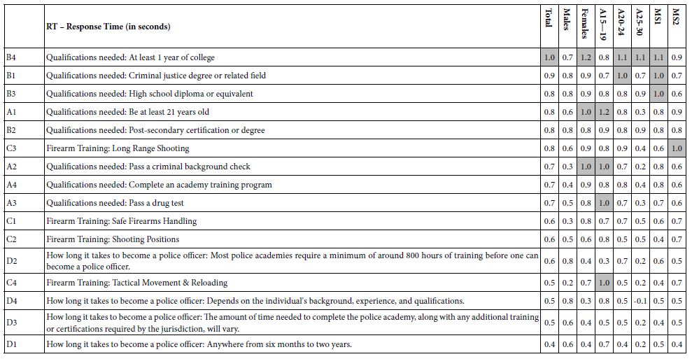
We finish the presentation of results and the analysis by considering the data from the point of view of response time (RT). Response time occupies a special position in psychology and consumer / public opinion research [15]. It is presumed by some reearchers that a lot can be learned by measuring ‘responses’ that cannot be consciously controlled. Response time to the stimulus is one of these measures, albeit very closely related to the stimulus, and thus a reasonable choice for a non-conscious measure, one step beyond the direct rating which is assumed to be a conscious measure measure.
Table 7 shows the coefficients from the group-level equations relating response time (RT) to the presence/absence of the 16 elements. As noted above, the equation is estimated without an additive constant. In ‘regression speak’ this is known as ‘forcing the equation through the origin.’ All coefficients 1.0 seconds or longer are shown in shaded cells. Finally, the table shows the elements sorted by decreasing response time.
There are some clear patterns emerging from Table 6, patterns which make sense,
There is a clear hierarchy of response times
B4 Qualifications needed: At least 1 year of college 1.0
D1 How long it takes to become a police officer: Anywhere from six months to two years. 0.4
There is one element, B4, which is consistently among the longest in every group, suggesting that the respondents think about this element. This element reads: Qualifications needed: At least 1 year of college.
In contrast, the elements dealing with ‘how long it takes to become a police officer’ generate the shortest response times among all groups.
The practical aspects of the response time data emerge when we think about the implications. If the objective is to convey relevant information, long response times are important. They figuratively ‘stop the reader in her/his tracks,’ engaging the reader. The information is important to the reader, forcing the reader to think about what was read.
Table 7: Coefficients for equations relating response time (RT) to the presence/absence of the 16 elements
Discussion and Conclusions
A glance through the various references suggest that researchers are aware of the need to understand careers from the mind of students [16,17], but often approach the issue from the ‘top down.’ That is, the researcher is the adult, asking the younger person about ‘why did you want to become a police officer?’ The top-down approach is hallowed in research, with the topic-experts investigating the topic at a distance.
What is missing from the foregoing approach is a sense of what the young person is thinking. The young person can only respond to questions formulated by individuals who are ‘outside’ them, probing them to understand how the young person thinks. One need only look at the published research about young people and police to realize that virtually all information is top-down [18,19].
This paper has presented a novel way to understand how young people think about a career. The novelty comes from the use of young people as researchers, as well as using other young people as respondents. The scientific community is accustomed to researchers being topic-experts, focusing their inquiry into a problem, after having formulated hypotheses.
The ability to make students into researchers emerges from the combination of a research approach (experimental design), coupled with a templated approach guiding the user (www.BimiLeap.com, embodying Mind Genomics), and with artificial intelligence to suggest ideas (Idea Coach). The result of this happy combination is that virtually any young person who can read and understand instructions can become a researcher. The benefit is that the topic can be investigated by those who are also most heavily involved. The researcher needs not be mature, nor be a topic expert. As long as the researcher knows what to do, the approach is straightforward. The technology is set up so that no adult has to be involved, either in the design of the study, or in the completion of the study. That simplification, allowing anyone to become a researcher, opens the possibility of far deeper understanding of the way children think, not so much from better theory as from the ability to give the mind of the child a way to explore topics in the form of an experiment, with answers from other qualified respondents appropriate to the study.
References
- Barthe EP, Leone MC, Lateano TA (2013) Commercializing success: The impact of popular media on the career decisions and perceptual accuracy of criminal justice students. Teaching in Higher Education 18: 13-26.
- Fekjær SB (2014) Police students’ social background, attitudes and career plans. Policing: An International Journal of Police Strategies & Management 37: 467-483.
- Howard KA, Walsh ME (2010) Conceptions of career choice and attainment: Developmental levels in how children think about careers. Journal of Vocational Behavior 76: 143-152.
- Kupchik A, Curran FC, Fisher BW, Viano SL (2020) Police ambassadors: Student‐police interactions in school and legal socialization. Law & Society Review 54: 391-422.
- Powell MB, Skouteris H, Murfett R (2008) Children’s perceptions of the role of police: a qualitative study. International Journal of Police Science & Management 10: 464-473.
- Sindall K, McCarthy DJ, Brunton-Smith I (2017) Young people and the formation of attitudes towards the police. European Journal of Criminology 14: 344-364.
- Moskowitz HR, Gofman A, Beckley J, Ashman H (2006) Founding a new science: Mind genomics. Journal of Sensory Studies 21: 266-307.
- Moskowitz HR, Gofman A (2007) Selling Blue Elephants: How to Make Great Products that People Want Before Theu Even Know They Want Them. Pearson Education.
- Gabay G, Moskowitz HR (2015) Mind Genomics: What Professional Conduct Enhances the Emotional Wellbeing of Teens at the Hospital? Journal of Psychological Abnormalities in Children.
- Gofman A, Moskowitz HR, Mets T (2011) Marketing museums and exhibitions: What drives the interest of young people. Journal of Hospitality Marketing & Management 20: 601-618.
- Mukerjee R, Wu CF (2006) A Modern Theory of Factorial Design. New York: Springer.
- Mendoza C, Deitel J, Braun M, Rappaport S, Moskowitz H (2023) Empowering Young Researchers: Exploring and Understanding Responses to the Jobs of Home Aide for a Young Child. Pediatric Studies and Care 3: 1-9.
- Gofman A, Moskowitz H (2010) Isomorphic permuted experimental designs and their application in conjoint analysis. Journal of Sensory Studies 25: 127-145.
- Likas A, Vlassis N, Verbeek JJ (2003) The global k-means clustering algorithm. Pattern Rrecognition 36: 451-461.
- Bassili JN, Fletcher JF (1991) Response-time measurement in survey research a method for CATI and a new look at nonattitudes. Public Opinion Quarterly 55: 331-346.
- Clinkinbeard SS, Solomon SJ, Rief RM (2021) Why did you become a police officer? Entry-related motives and concerns of women and men in policing. Criminal Justice and Behavior 48: 715-733.
- Durkin K, Jeffery L (2000) The salience of the uniform in young children’s perception of police status. Legal and Criminological Psychology 5: 47-55.
- Ho T (1999) Assessment of police officer recruiting and testing instruments. Journal of Offender Rehabilitation 29: 1-23.
- Kanable R (2001) Strategies for recruiting the nation’s finest. Law Enforcement Technology 28: 64-68.