DOI: 10.31038/IMCI.2019222

Abstract

Brain volumes of 73 infants, children, and adolescents were determined in three planes (sagittal, axial, coronal) using ImageJ, and these were then compared separately and collectively to those obtained using simple linear measurements. The “R” package was used for statistical analyses. Correlations were strong for all measured and measured to calculated comparisons, with r values of 0.87 – 0.93 (p <0.001).  Correlation of measured right and left cerebral hemispheric volume (means = 450 and 458 cm³, respectively) was r = 0.94 (p <0.001), and measured compared to calculated right or left cerebral hemispheric volumes were r = 0.90 and 0.86, respectively (p <0.001). The left cerebral hemisphere was greater in 43/73 (58%) brains. There was no correlation between the extent of the hemispheric volume percent differences or side to side asymmetries and age (r = -0.11; p = 0.34). The results indicate that calculated measurements of brain and cerebral hemispheric volumes are near identical to respective measurements obtained with ImageJ. The findings justify the use of linear measurements as a means of calculating regional and global brain volumes

Keywords

brain, development, ImageJ, linear measures, MRI

ImageJ (NIH image-processing program FIJI) is a widely available and frequently used software process to directly obtain a variety of regional and global measurements, including distances, areas, and volumes in multiple tissues and organs [1–6]. The image analysis program recently has been updated to allow for a more diverse and user friendly audience [7]. The brains of animals, including humans, has been extensively studied, both in vitro and in vivo [1–3, 5, 6]. However, few investigations have been accomplished to study macro- and micro-structural aspects of the brain during development [8]. Th major objective of the present investigation was to ascertain developmental aspects of brain growth in human infants, children, and adolescents using ImageJ and to compare the results to those obtained from the use of linear measurements. We have previously employed the latter method to estimate total brain volume as well as aspects of cerebral hemispheric asymmetry and corpus callosal structure [9–12]. The results of the correlative study authenticate the utility of using multiple linear measures and appropriate formulations to determine regional and global areas and volumes of the brain in health and disease [13].

Materials and Methods

Study Cohort

The sampled population included pediatric patients evaluated and managed by neurological, neurosurgical, and other personnel at the Weil Cornell Medical Center (WCMC) in New York, NY. A total of 73 individuals from a larger cohort of 123 patients was selected, each of whom had undergone a brain MRI scan for one of several reasons, and whose scan was interpreted as “normal” by a neuroradiologist, under the directorship of LAH. Eight individuals were 6 – 18 years of age, while the ages of the remaining 65 patients ranged from near birth to six years. Approximately 12 subjects (6 females; 6 males) were selected from each of the following age categories: 1 – 6, 7 – 12, 13 -18, and 19 – 24 months; 2 – 4, and 5 – 6 years. As discussed previously [9], these age categories were chosen to match the period of maximal brain expansion during the early years of postnatal development. Brain expansion is 95% complete by six years of age [9]. All patients were selected from the electronic files of WCMC, extending from January, 2013 through June, 2018. Inclusion criteria included: 1) birth through 18 years; 2) a brain MRI that was interpreted as normal; and 3) an occipto-frontal (head) circumference (OFC) above the fifth percentile for age and sex. Exclusion criteria included: 1) fetuses; 2) premature infants less than 36 weeks gestation with evidence of brain damage; 3) age equal to or greater than 19 years; 4) abnormal MRI scans, excluding normal variants; or 5) absent clinical information. To obtain an equal sex and age distribution in accordance with the age-specific categories (see above), eligible patients were included in the study until each age category was filled with a near equal number of males and females. Thereafter, the MRI scans were retrieved from the electronic files and reviewed. Specific brain measurements then were obtained (see below).

Patient Confidentiality and Institutional Approval

The protocol encompassing the research plan was approved by WCMC Institutional Review Board on July 14, 2017. Given that all data collected were retrospective in nature, a “Waiver of Informed Consent” was approved.

MRI Imaging Protocol

All brain MRI examinations were performed with or without contrast enhancement on a 1.5 or 3.0 T General Electric (GE Medical Systems, Milwaukee, Wisconsin) whole-body imager equipped with high performance gradients and a manufacture-supplied quadrature head coil. Whole brain 3 dimensional T2 weighted localizers, sagittal T1 and axial T1-weighted, T2-weighted, T2-FLAIR, and diffusion wighted images were routinely collected on all subjects at a maximum of 5 mm and a minimum of 1 mm thickness (the majority at 3 mm). To maximize proper alignment, the patients’ heads were positioned in the midline with the aid of a laser centering device focused on the nose, philtrum, and chin.  The axial acquisition of the brain was acquired parallel to the hard palate or parallel to a line joining the anterior and posterior commissures, while the coronal acquisitions were obtained perpendicular to the axial acquisition. All scans were performed for clinically indicated reasons. Infants under the age of 12 months were often fed, swaddled, and scanned without sedation. Despite these maneuvers, some infants required sedation for optimal image acquisition.

Measurements of Brain Volume

To measure brain volume in each of three planes (sagittal, axial, coronal), a modification of the Cavalieri principle was applied to sequential images selected from the Cornell database [1,4]. Between 12 and 18 equidistant images were selected depending upon the total number of images in each plane, ranging from 30 to 178. Screenshots of the entire squares with included images then were obtained and appropriately labeled for individual, dataset, and plane identification. The sets of screenshots then were placed into separate folders also labelled with the dataset number and the plane. Maximal brain length and height were recorded on a near mid-line sagittal image. The height measurement extended from the vertex to the level of the foramen magnum. Maximal length and width also were recorded on an axial image at the level of the frontal horns of the lateral ventricles. Lastly, maximal width and height were recorded on a coronal image at the level of the full appearance of the brain stem. The average of the length measurements was used for the total distance of the collective coronal images, the average of the width measurements for the sagittal images, and the average of the height measurements for the axial images.

Using ImageJ, the MRI images containing the linear measurements were inserted to ascertain their respective distances as determined by the algorithm. The values for these distances were then divided by their respective distances recorded on the screenshots, which resulted in two conversion ratios for each of the three planes. The two ratios from each plane then were averaged and ultimately applied to the calculation of brain volume in each of the three planes. Thereafter, the areas in cm² for all the images in a single plane were determined using manual planimetry in ImageJ. The values were then added together and divided by the total number of images including the empty ones at the beginning and end of the series [1]. Thus, the average area of the entire series of images was obtained. The averaged area was then divided by the plane conversion ratio squared. The result was then multiplied by the maximal distance in cm to obtain the brain volume in cm³. As previously described, for the sagittal brain volume determination, the maximal width was used; for the axial volume, the maximal height determination was used; and for the coronal volume, the maximal length determination was used. Cerebral hemispheric volumes were determined in a similar manner using only the sagittal images. To ascertain the optimal number of measured images in each plane, a preliminary study was conducted on a single brain (#4). This individual was an 18 year old male, with a height of 182 cm (6.0 feet), a weight of 83 kg (183 lbs), and an occipito-frontal (head) circumference of 53 cm. There were a total of 43 axial images. The following brain volumes were ascertained using various numbers of areas in the volume calculations:

Eighteen and 12 brain images produced brain volumes that were 98 and 96%, respectively, of the brain volume using 43 images. Therefore, between 12 and 18 of the total number of images were assumed to provide a near perfect estimate of overall brain volume [4].

Calculation of Brain Volumes

The other method to determine total brain volume utilized a combination of linear craniometric measurements, which incorporated brain length, width, and height. This method has been described previously as well as the rationale for its use [9, 12–13]. Brain length measures included SCL, FCP, and ACL; brain width measures included AFQ, ASQ, and ATQ; and brain height measures included SFQ, SSQ, and STQ [9]. The component measures of length, width, and height were individually averaged to provide equal weighting of the three dimensions.  Total brain volume was then calculated according to the elliptical equation:

Brain volume (cm³) = (4/3) × pi (3.14) × r (length) × r (width) × r (height)

An adjustment equation was then applied to the volume measurements (Vannucci et al, 2019b):

Adjusted brain volume = (calculated brain volume × 1.2) + 11

For the calculated cerebral hemispheric volumes, the length measurements were ACLr1 and ACLr2, the width measurements were AHR, ASQr, and PHR for the right cerebral hemisphere, and a single coronal height measurement was CRH [11] Comparable “l” designations were determined for the left cerebral hemisphere. As with the whole brain measurements, an adjusted equation was applied to the cerebral hemispheric volume measurements (see above).

Data Analysis

The collected and tabulated data were subjected to statistical analyses by use of correlation and linear regression methods. Both predictor and response variables included the measured brain and cerebral hemispheric volumes in the sagittal, axial, and coronal planes, while other response variables included the calculated brain volume measurements. Two sample t tests also were performed. All statistical tests were performed and graphics produced using “R” software [14].

Results

The volumes of 73 brains were analyzed with ImageJ in the sagittal and axial planes and of 69 brains in the coronal plane. Table 1 shows the relationships between the three measured (ImageJ) variables, where the three correction coefficient (r) values were highly significant at 0.88 – 0.89 (see also Figure 1). Table 1 also shows the relationships between the brain volumes derived from the three separate planes and the combined volumes compared to the calculated brain volumes (see also Figure 2). All relationships were highly statistically significant (p<0.001), with r values ranging from 0.88 to 0.94, and slopes very close to 1.00. Right and left cerebral hemispheric volumes were measured in the 73 brains, with larger left hemispheres in 43 (58%) specimens (Figure 3a). One brain showed an identical hemispheric volume, while 11 brains possessed hemispheres with less than 10 cm³ difference (15%). Sixteen brains showed at least a 50 cm³ difference (22%), while only one brain showed greater than a 100 cm³ difference. The mean volume of the right cerebral hemisphere was 450 cm³, while that of the left hemisphere was 458 cm³, an overall 8 cm³ difference (p = 0.12). There was no correlation between the extent of the measured hemispheric volume differences or side-to-side asymmetries and age (r = -0.11; p = 0.34) (Figure 3b), which was also the case for calculated hemispheric volume differences and age (r = -0.12; p = 0.33). There was also no correlation between the extent of the hemispheric volume differences and calculated brain volume (r = -0.09; p = 0.46). Each measured cerebral hemispheric volume was then correlated with its respective calculated hemispheric volume (Table 1; Figures 3c and d). The percent difference between the measured and calculated right cerebral hemispheric volume ranged from 66 to 119%, with a mean of 97% (p = 0.15) (Figute 3e). The percent difference between the measured and calculated left cerebral hemispheric volume ranged from 60 to 125%, with a mean of 102% (p = 0.06) (Figure 3e).

Figure 1a

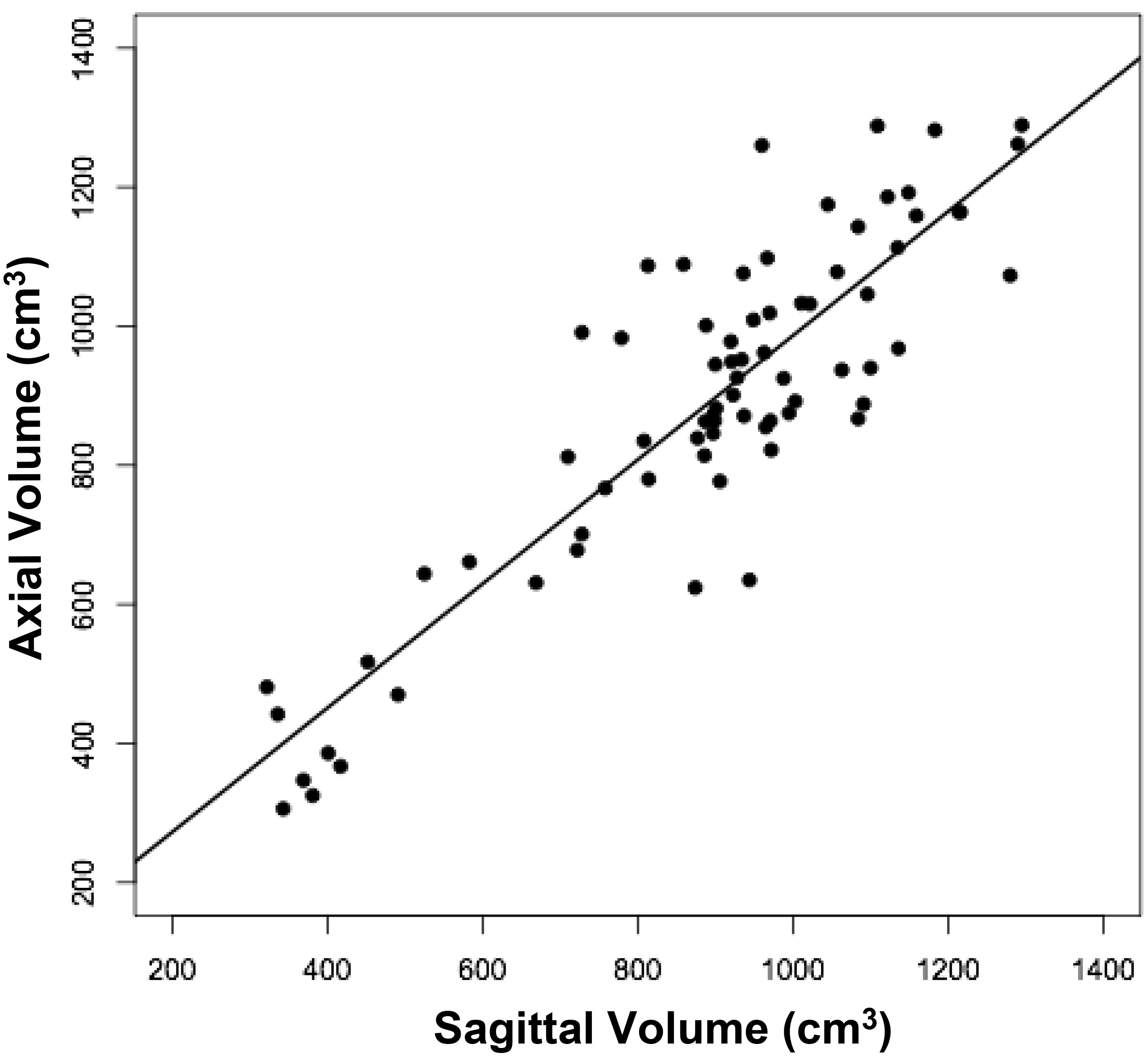
Figure 1b

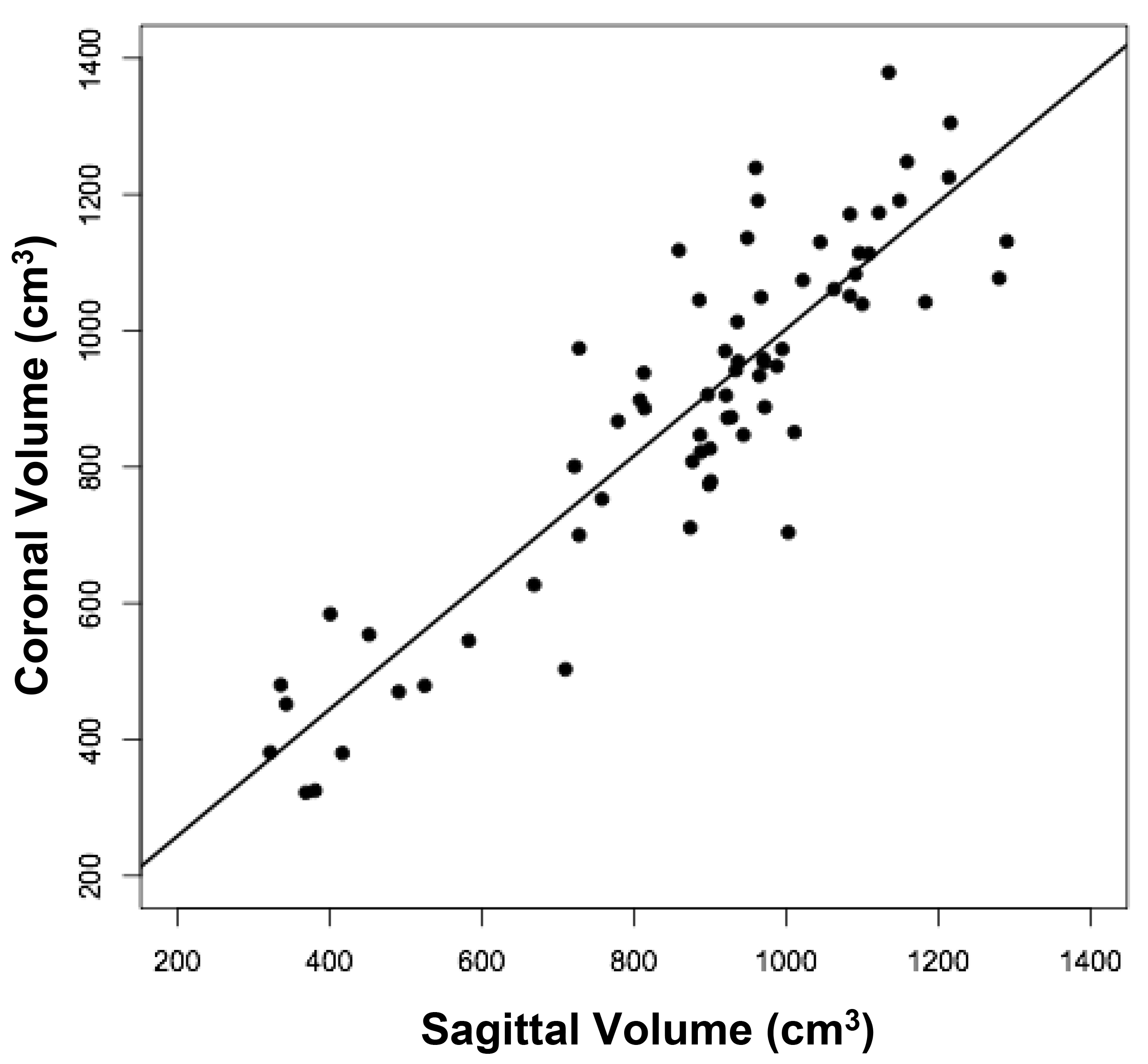
Figure 1c

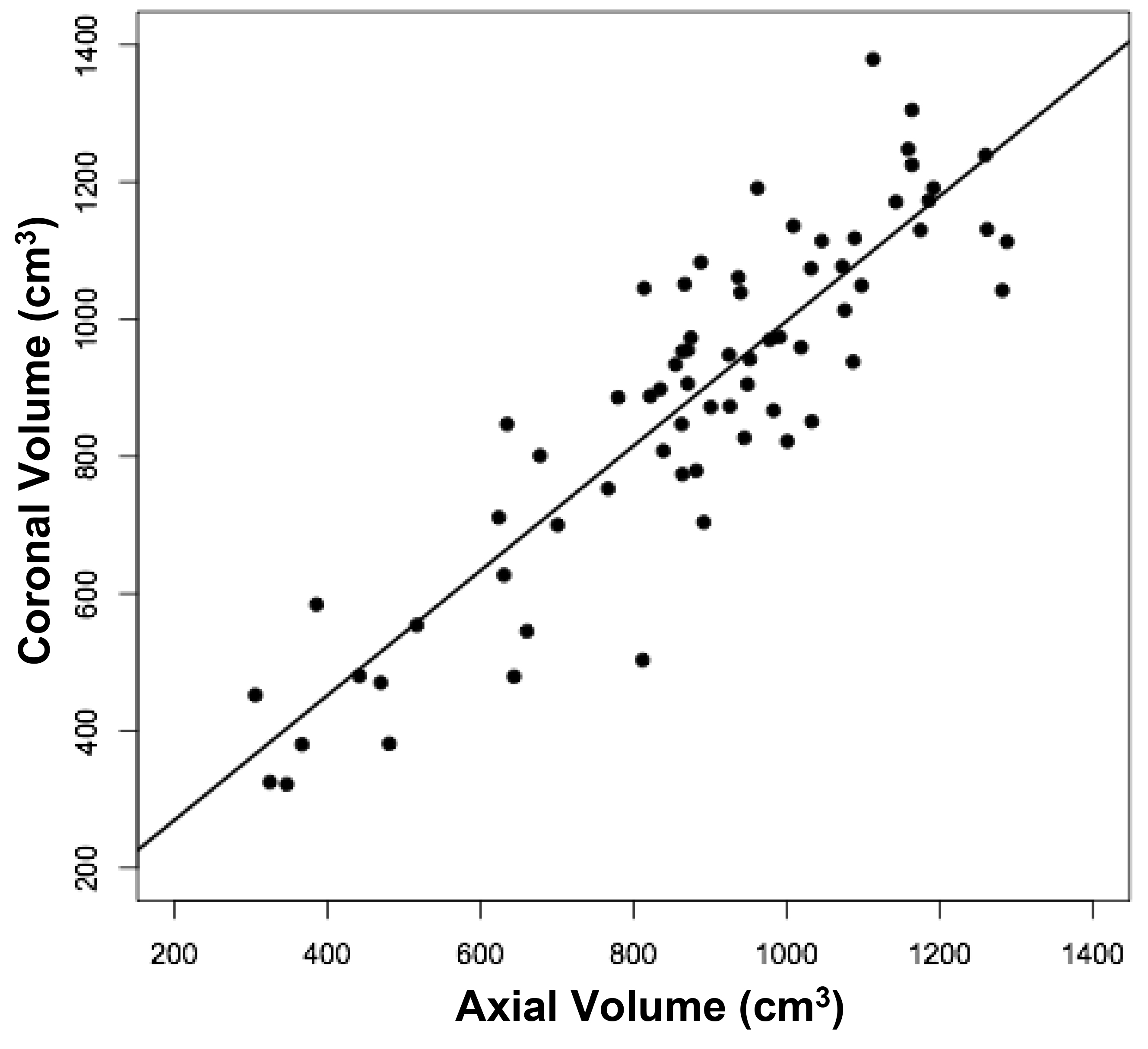
Figure 1. Relationships between measured brain volumes in the sagittal, axial, and coronal planes.

Shown are linear regression plots, each comparing two of the three variables. Regression lines are shown. The correlation coefficient (r) and probability (p) values are shown in Table 1.

Table 1. Linear Regression Relationships between Measured and Calculated Brain Volumes.

The first variable is x, while the second variable is y.

Figure 2a

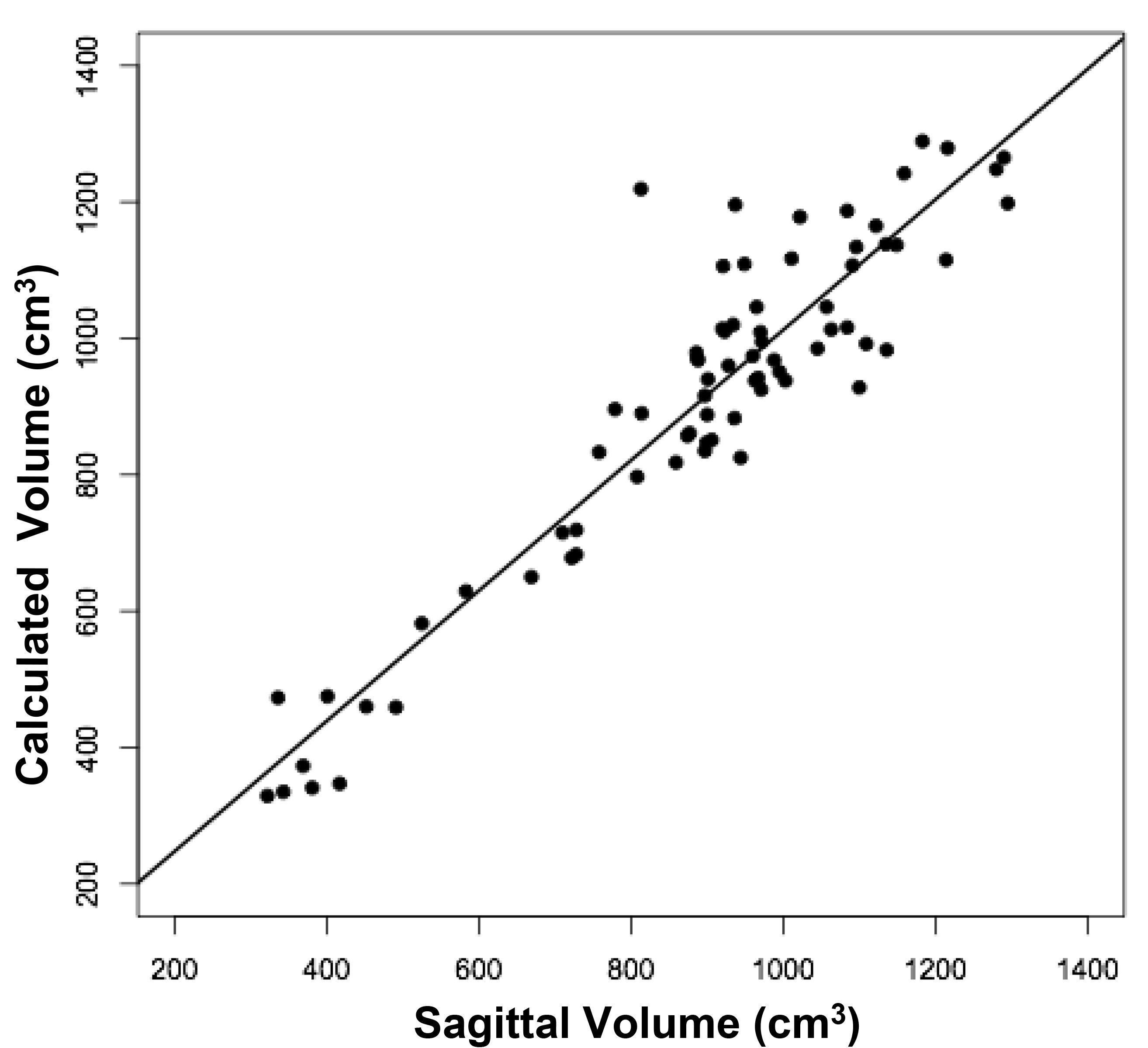
Figure 2b

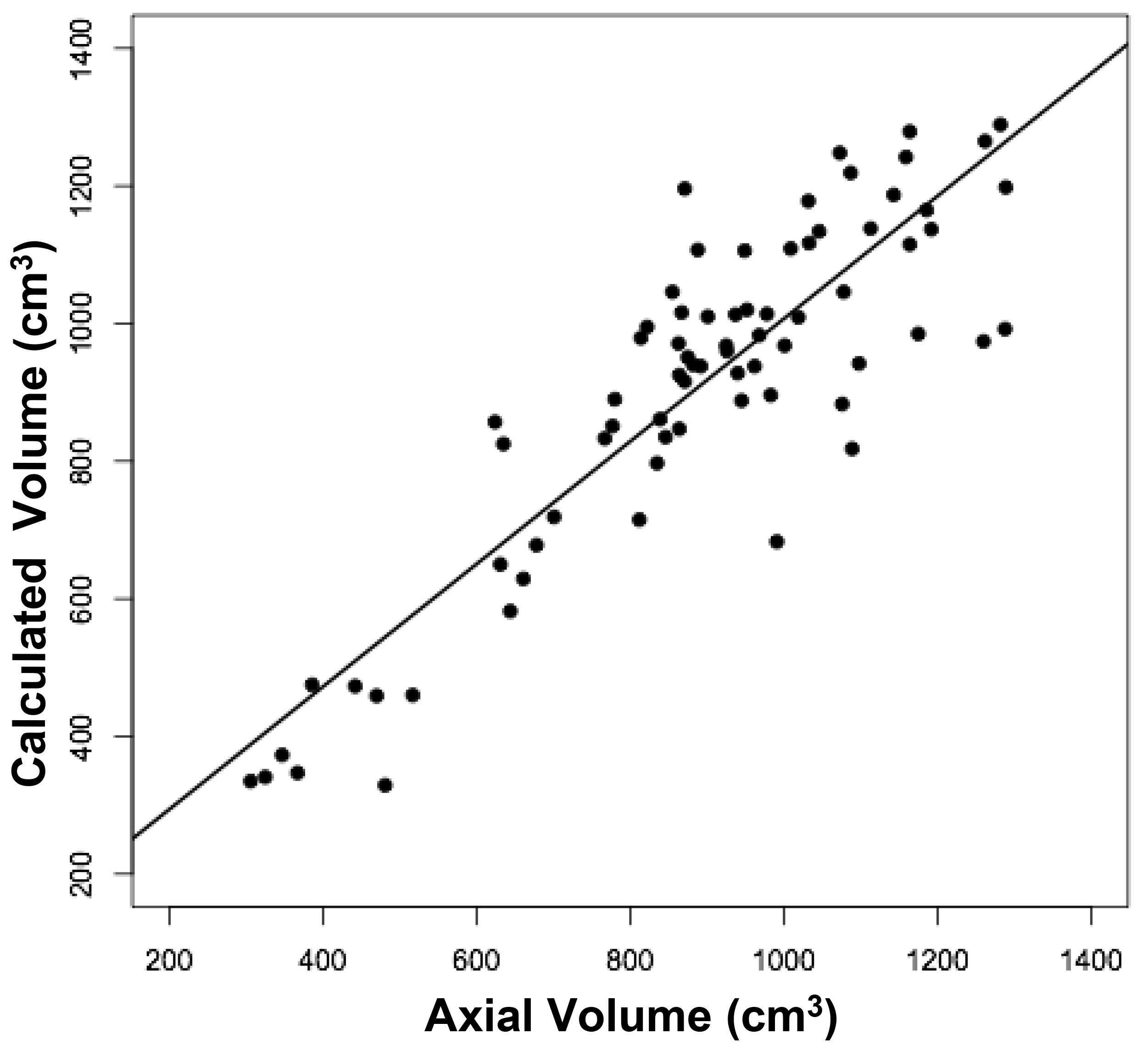
Figure 2c

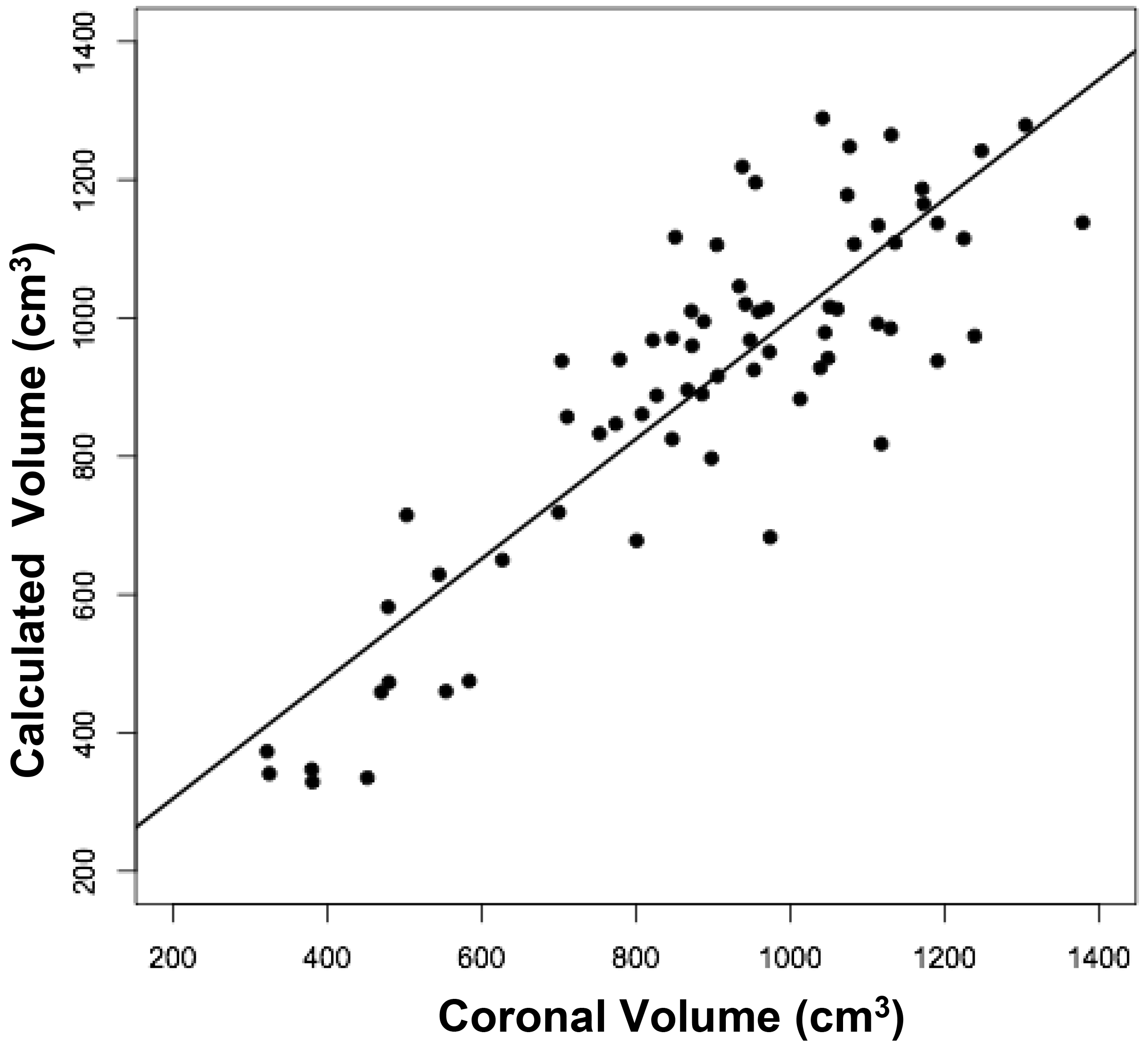
Figure 2d

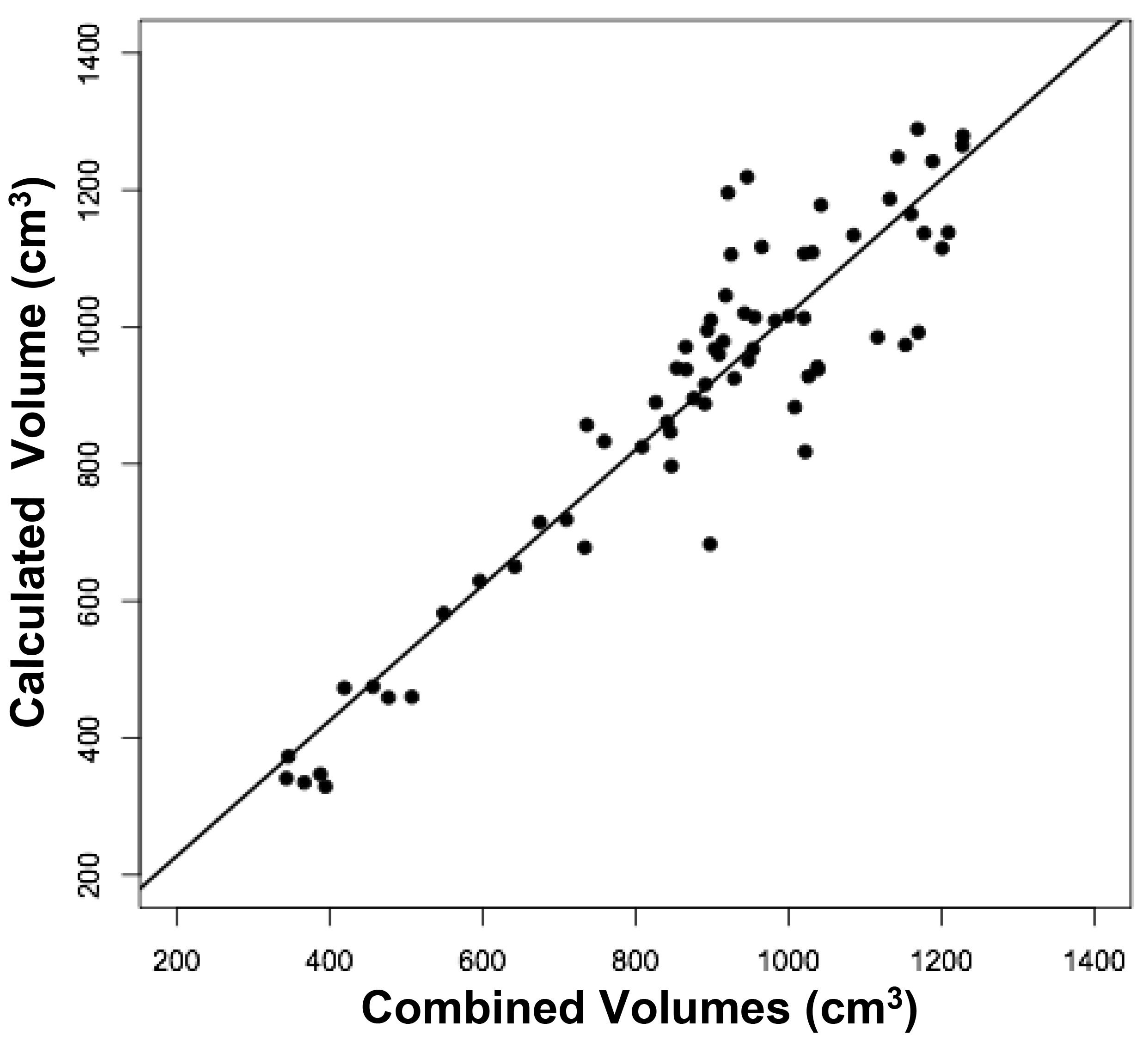
Figure 2. Relationships between measured brain volumes and calculated brain volume.

Shown are linear regression plots, each comparing one of the three measured variables to the cal-culated variable.  Regression lines are shown.  The correlation coefficient (r) and probability (p) values are shown in Table 1.

Figure 3a

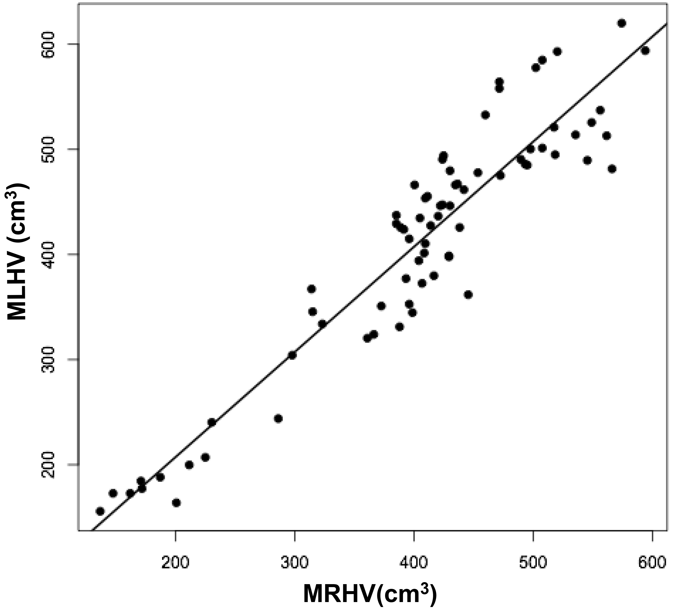
Figure 3b

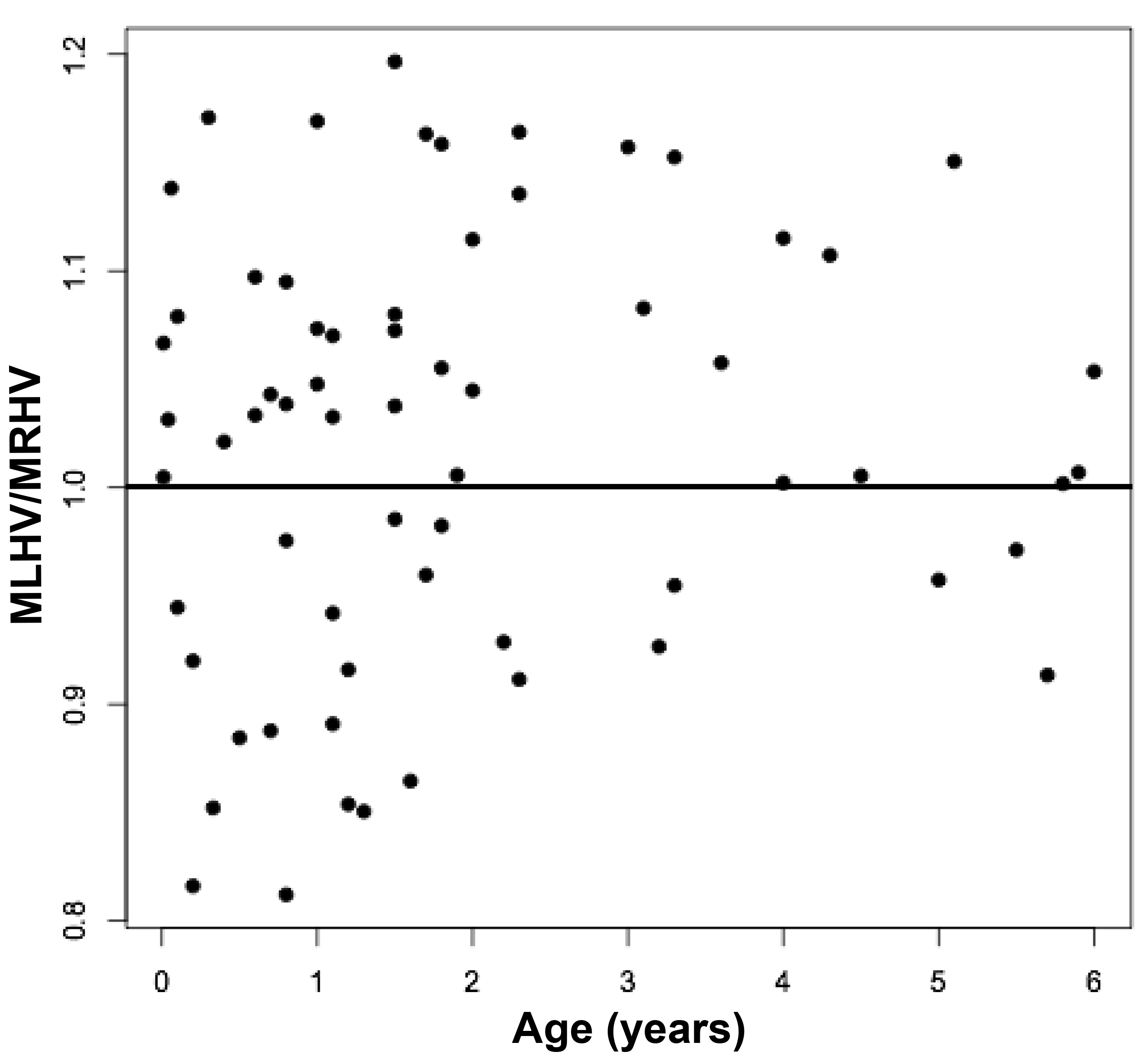
Figure 3c

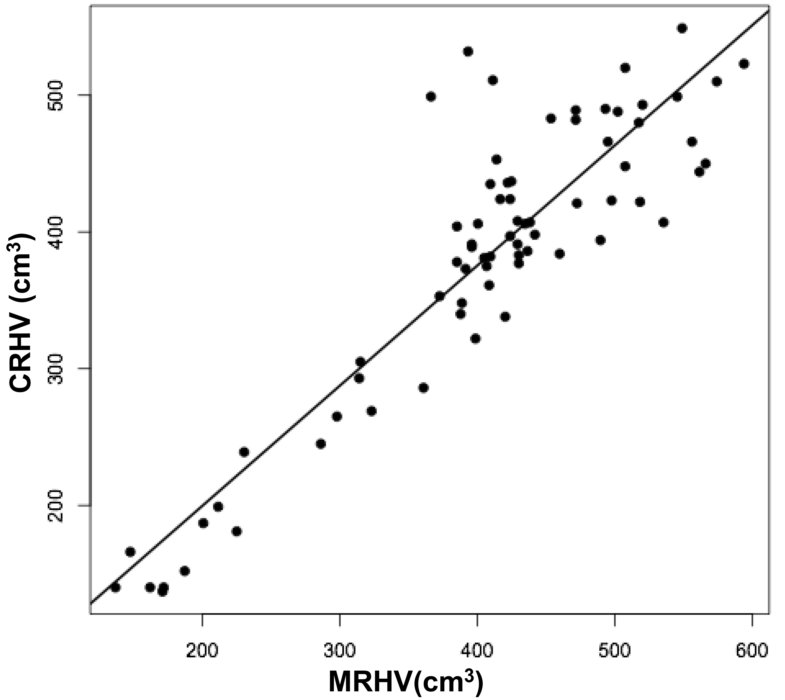
Figure 3d

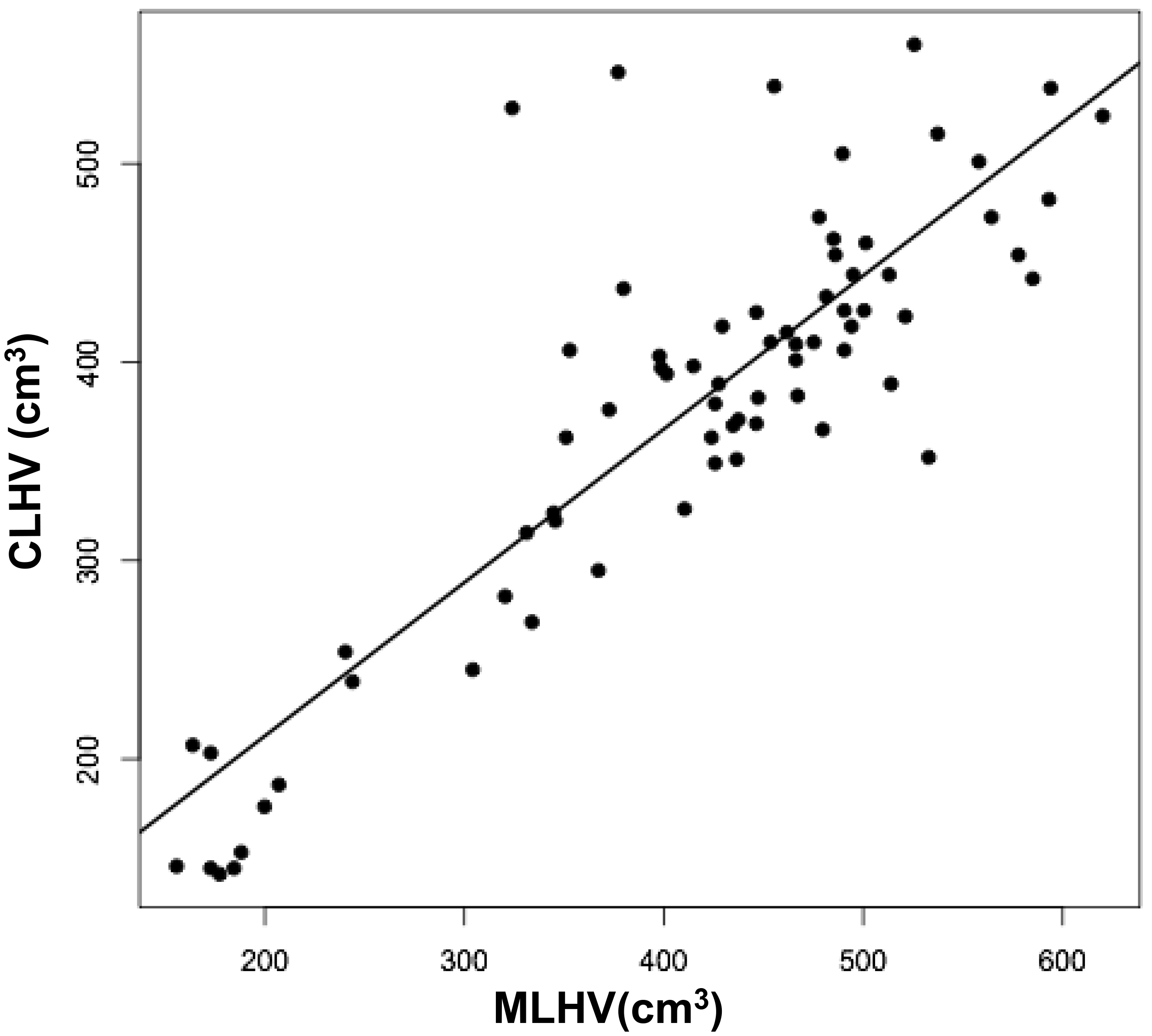
Figure 3e

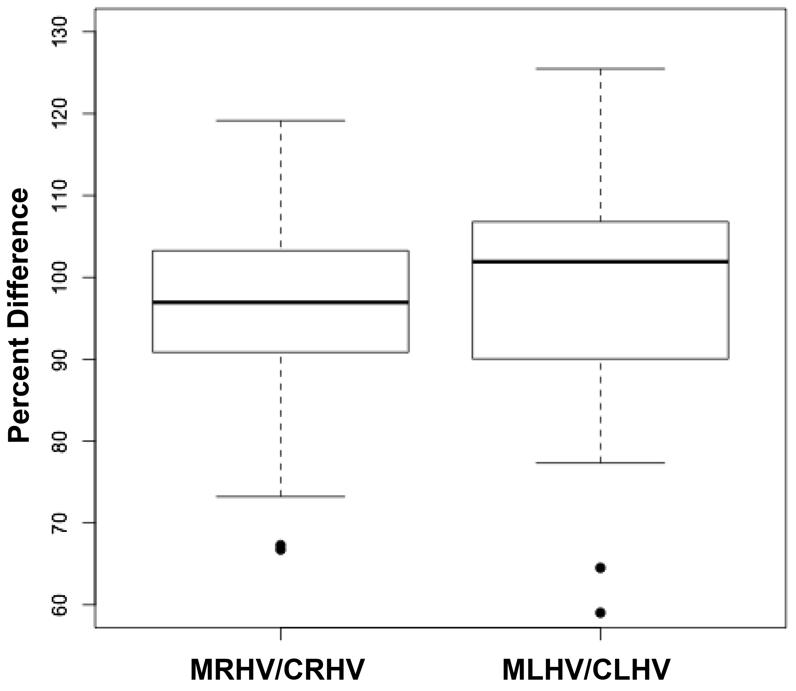
Figure 3. Relationships between measured and calculated right and left cerebral hemispheric volumes.

Figures 3 a, c, and d are linear regression plots, each comparing the measured variables to each other and to their respective calculated variables.  Regression lines are shown.  The correlation coefficient (r) and probability (p) values are shown in Table 1.  Figure 3b correlates MLHV/MRHV with age to six years.  The horizontal line distinguishes the larger of the two hemispheres; MLHV above and MRHV below the line.  Figure 3e shows  boxplots of MRHV/CRHV and MLHV/CLHV.  The circles are outliers.

Abbreviations: MRHV, measured right cerebral hemispheric volume; MLHV, measured left cer-ebral hemispheric volume; CRHV, calculated right cerebral hemispheric volume; CLHV, calcu-lated left cerebral hemispheric volume.

The measured brain volumes were then correlated with age through seven years (Figure 4). The most dramatic increase in brain size occurs between birth and 18 months, with little further change thereafter. Such age related changes in brain size previously have been observed in the present and other cohorts of infants, children, and adolescents [9, 15]. Comparisons between measured and calculated brain volumes in different age groups were similar. Brain sizes in infants aged near birth to six months were 498 and 504 cm³, respectively (p = 0.95), while the sizes in infants aged 13 – 18 months were 931 and 961 cm³, respectively (p = 0.54), and in children aged 5 – 6 years were 1,092 and 1,145 cm³, respectively (p = 0.17).

Figure 4a

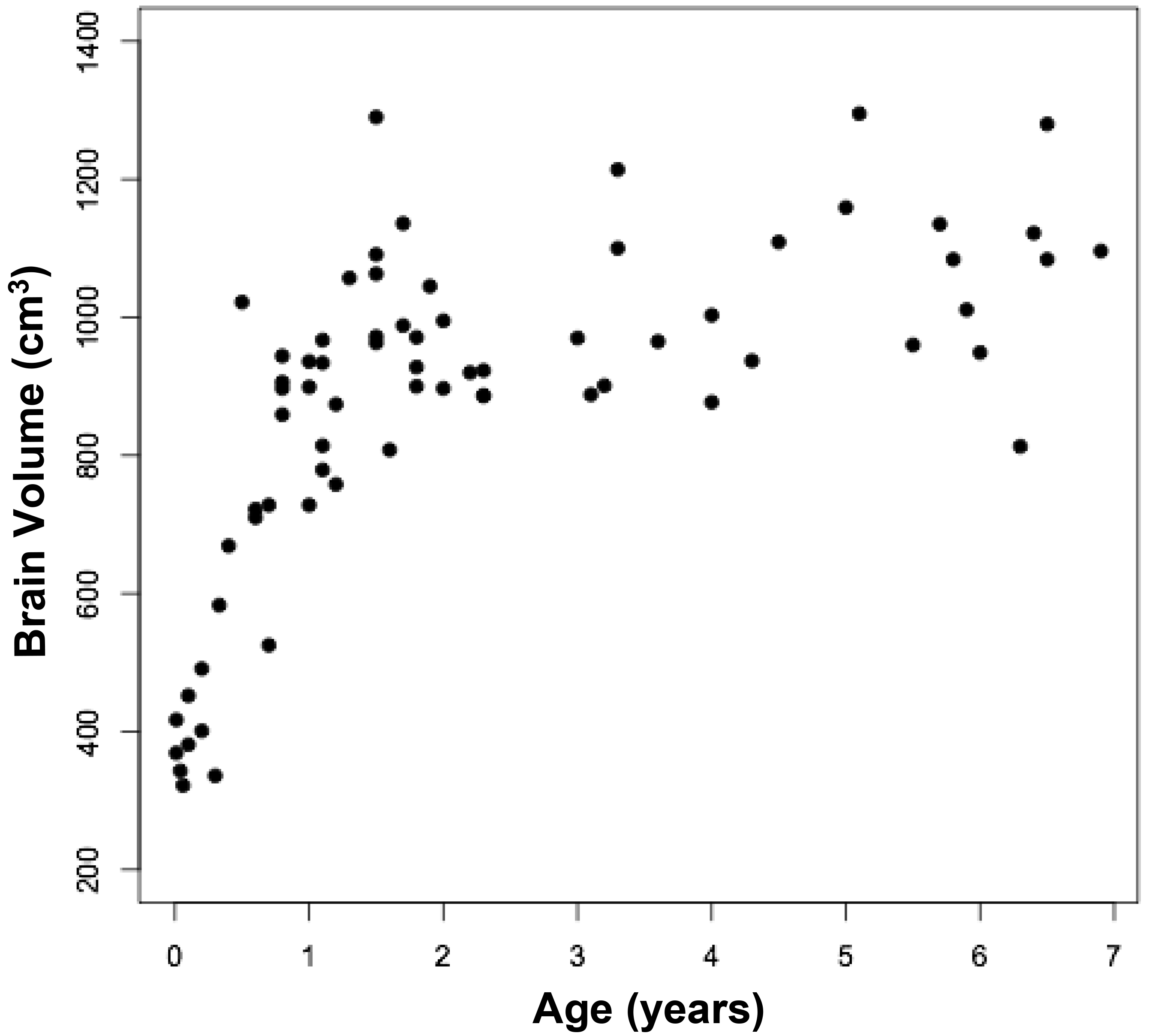
Figure 4b

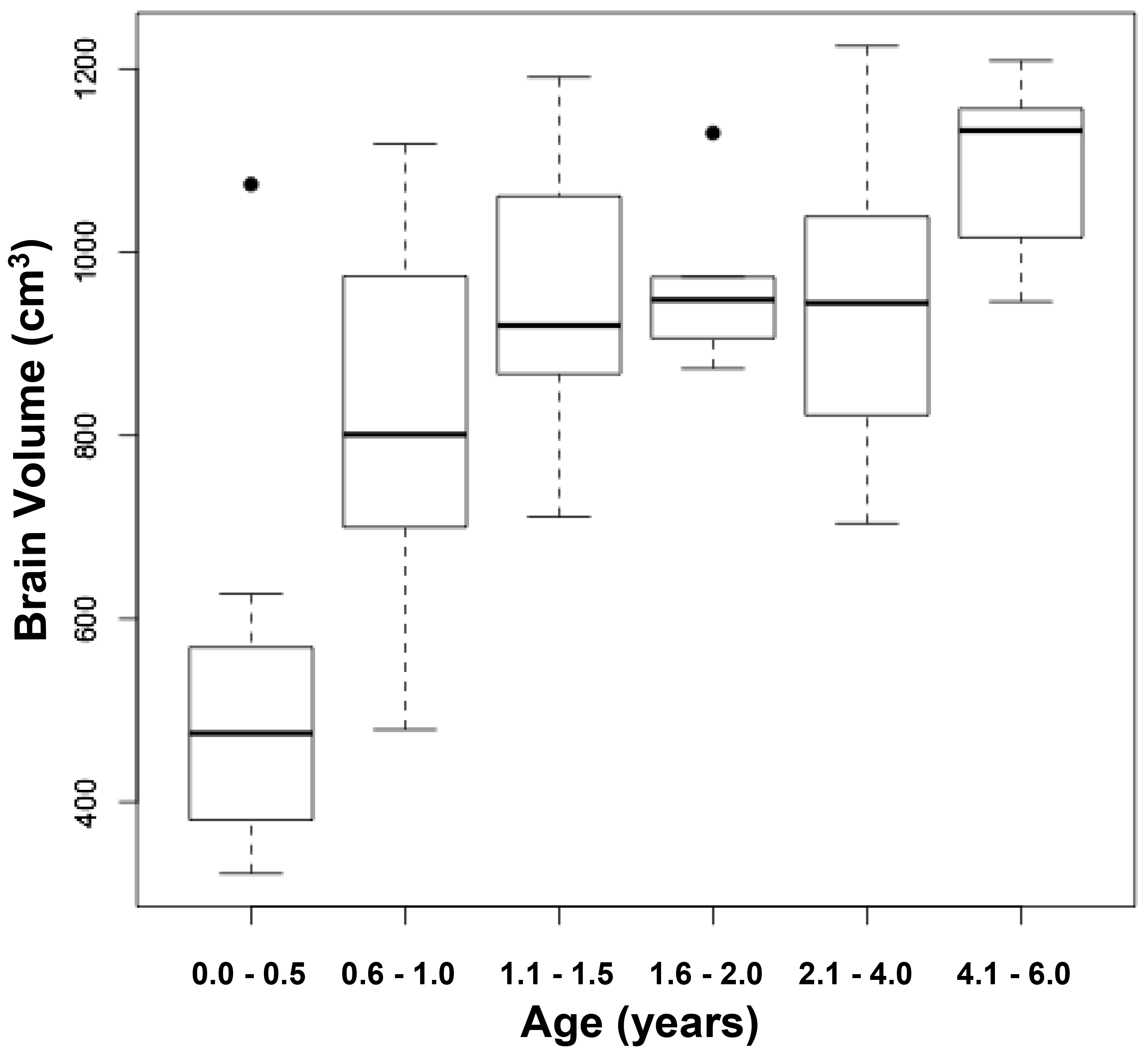
Figure 4. Relationship between measured brain volumes and age.

Figure 4a represents a scattergram, while figure 4b represents boxplots at different ages.  The circles are outliers.

Discussion

The results of the present investigation serve several purposes. Firstly, the brain volumes measured in three separate planes were similar, providing justification for the use of ImageJ and our described procedure to obtain the individual volumes. Secondly, the measured and calculated brain volumes also were similar, providing additional justification for the use of linear measurements as a means of calculating regional and global brain volumes [9,12]. The measured and calculated cerebral hemispheric volumes were less similar, although the majority of the comparisons were within 90% of each other (Figure 3d). Accordingly, calculated measurements of brain and cerebral hemispheric volume are near identical to those of measurements obtained with ImageJ. As in the present study, we previously have examined side to side differences in calculated total cerebral hemispheric volume and found no consistency throughout development, although on a regional basis, the right frontal and left occipital lobes are wider than their left or right counterparts [11]. Right frontal and left occipital protrusions (petalias) also are present in the majority of individuals during development to complement the regional differences. Several other studies have addressed the issue of cerebral hemispheric asymmetries, most or all of which are discussed in Vannucci et al. [11].

There are numerous studies that utilize technologically advanced, computational methods to orient, visualize and measure cerebral hemispheric volumes and shapes as well as gray/white matter and gyral/sulcal patterns [16–21]. Frequently used techniques are Deformation-Based Morphometry (DBM), Tensor-Based Morphometry (TBM), and Voxel-Based Morphometry (VBM) [18, 20, 22, 23]. These methods have both advantages and limitations. The advantages relate to the investigators’ ability to properly orient the brain, to erode unwanted structures (e.g. skull, CSF, ventricles), and then to parcellate specific regions for comparative analyses. The limitations relate to the requirement for multiple steps in pre-processing, processing, normalization, and segmentation; which can reduce anatomical specificity. Thereafter, complex analytical assumptions (e.g. gaussian or Bayesian models) must be met in order for accurate global or regional comparisons to be made. In the present investigation, we found that our previously used simple linear measurements to ascertain regional and global brain volumes closely approximate those measured with one such advanced analytical technique, specifically Image [9, 10]. The method also allows for very accurate inter-hemispheric comparisons, so long as the MRI images are in proper alignment [11].

Acknowledgement

The authors thank Dr. Barry Kosoksky and his associates in the Department of Pediatrics (Child Neurology) and other members of the WCMC physician faculty for allowing us to obtain the clinical files of their patients.

Ethical Approval; Conflicts Of Interest; Funding

All procedures performed in our study involving human participants were in accordance with the ethical standards of the institutional and/or national committee and with the 1964 Helsinki declaration and its later amendments or comparable ethical standards. As indicated in Materials and Methods, the present human research effort was approved by the Weil Cornell Medical Center Institutional Review Board on July 14, 2017. Since the collection of data was retrospective in nature, a “waiver of informed consent” was approved.

This research did not receive any specific grant from funding agencies in the public, commercial, or not-for-profit sectors.

Abbreviations: SV, ImageJ sagittal volume, AV, ImageJ axial volume; CV, ImageJ coronal volume; CBV, calculated brain volume; comb., combined; MRHV, measured right cerebral hemispheric volume; MLHV, measured left cerebral hemispheric volume; CRHV, calculated right cerebral hemispheric volume; CLHV, calculated left cerebral hemispheric volume.

Reference

1. García-Fiñana M, Cruz-Orive LM, MacKay CL, Pakkenberg B, Roberts N (2003) Comparison of MR imaging against physical sectioning to estimate the volume of human cerebral compartments. NeuroImage 18: 505–516.
2. Pool M, Thiemann J, Bar-Or A, Fournier AE (2008) Neurite tracer: a novel ImageJ plugin for automated quantification of neurite outgrowth. J Neurosci Methods 168: 134–139.
3. Brabec J, Rulseh A, Hoyt B, Vizek M, Horinek D, et al. (2010) Volumetry of the human amygdala – an anatomical study. Psychiatry Res 182: 67–72.
4. Sahin B, Elfaki A (2012) Estimation of the volume and volume fraction of brain and brain structures on radiological images. NeuroQuantology 10: 87–97.
5. Paletzki R, Gerfen CR (2015) Whole mouse brain image reconstruction from serial coronal sections using FIJI (Image J). Curr Protoc Neurosci 73: 1–21.
6. Young K, Morrison H (2018) Quantifying microglia morphology from photomicrographs of immunohistochemistry prepared tissue using ImageJ. J Vis Exp doi: 10.3791/57648.
7. Rueden CT, Schindelin J, Hiner MC, DeZonia BE, Walter AE, (2017) ImageJ: ImageJ for the next generation of scientific image data. BMC Bioinformatics 18: 529 (1–26).
8. Khalsa SS, Geh N, Martin BA, Allen PA, Strahle J, et al. (2018) Morphometric and volumetric comparison of 102 children with symptomatic and asymptomatic Chiari malformation Type I. J Neurosurg Pediatr 21: 65–71.
9. Vannucci RC, Barron TF, Lerro D, Antón SC, Vannucci SJ (2011) Craniometric measures during development using MRI. NeuroImage 56: 1855–1864.
10. Vannucci RC, Barron TF, Vannucci SJ (2017) Development of the corpus callosum: An MRI study. Develop Neurosci 39: 97–106.
11. Vannucci RC, Heier LA, Vannucci SJ (2019) a.  Cerebral asymmetry during development using linear measures from MRI. Early Human Develop. (in press).
12. Vannucci RC, Vannucci SJ (2019) b. Brain growth in modern humans using multiple developmental databases. Am J Phys Anthropol 168: 247–261.
13. Vannucci RC, Barron TF, Vannucci SJ (2012) Craniometric measures of microcephaly using MRI. Early Human Develop 88: 135–140.
14. R Development Core Team (2009) R: A language and environment for statistical computing. Vienna: The R foundation for Statistical Computing  http://www.R-project.org.
15. Vannucci RC, Vannucci SJ (2019) b. Brain growth in modern humans using multiple developmental databases. Am J Phys Anthropol 168: 247–261.
16. Foundas AL, Leonard CM, Heilman KM (1995) Morphologic cerebral asymmetries and handedness. Arch Neurol 52: 501–506.
17. Good CD, Johnsrude I, Ashburner J, Henson RNA, Friston KJ, (2001) Cerebral asymmetry and the effects of sex and handedness on brain structure: A voxel-based morphometric analysis of 465 normal adult human brains. NeuroImage 14: 685–700.
18. Hervé P-Y, Crivello F, Perchey G, Mazoyer B, Tzourio-Mazoyer N (2006) Handedness and cerebral anatomical asymmetries in young adult males. NeuroImage 29: 1066–1079.
19. Keller SS, Roberts N (2009) Measurement of brain volume using MRI: software, techniques, choices and prerequisites.  J Anthropol Sci 87: 127–151.
20. Lyttelton OC, Karma S, Ad-Dab’bagh Y, Zatorre RJ, Carbonell F, (2009) Positional and surface area asymmetry of the human cerebral cortex. NeuroImage 46: 895–903.
21. Narr KL, Bilder RM, Luders E, Thompson PM, Woods RP, (2007) Asymmetries of cortical shape: Effects of handedness, sex and schizophrenia. NeuroImage 34: 939–948.
22. Ashburner J, Friston KJ (2000) Voxel-based morphometry-The methods.  NeuroImage 11: 805–821.
23. Ashburner J (2009) Computational anatomy with the SPM software.  Mag Res Image 27: 1163–1174.