DOI: 10.31038/MIP.2021211

Abstract

Background and objectives: Allograft rejection is a major concern in kidney transplantation. Inflammatory processes in patients with kidney allografts involve various patterns of immune cell recruitment and distributions. Lymphoid aggregates (LAs) are commonly observed in patients with kidney allografts and their presence and localization may correlate with severity of acute rejection. Alongside with other markers of inflammation, LAs assessment is currently performed by pathologists manually in a qualitative way, which is both time consuming and far from precise. In this work we aim to develop an automated method of identifying LAs and measuring their densities in whole slide images of transplant kidney biopsies.

Materials and Methods: We trained a deep convolutional neural network based on U-Net on 44 core needle kidney biopsy slides, monitoring loss on a validation set (n=7 slides). The model was subsequently tested on a hold-out set (n=10 slides).

Results: We found that the coarse pattern of LAs localization agrees between the annotations and predictions, which is reflected by high correlation between the annotated and predicted fraction of LAs area per slide (Pearson R of 0.9756). Furthermore, the network achieves an auROC of 97.78 ± 0.93% and an IoU score of 69.72 ± 6.24% per LA-containing slide in the test set.

Conclusions: Our study demonstrates that a deep convolutional neural network can accurately identify lymphoid aggregates in digitized histological slides of kidney. This study presents a first automatic DL-based approach for quantifying inflammation marks in allograft kidney, which can greatly improve precision and speed of assessment of allograft kidney biopsies when implemented as a part of computer-aided diagnosis system.

Keywords

Kidney, Machine learning, Segmentation, Inflammation, Lymphoid aggregates

Introduction

End-to-end deep learning (DL) methods have approached human performance in multiple computer vision tasks [1,2] and have more recently been successfully utilized in many biomedical domains [3-5]. Convolutional neural networks (CNN) are a class of artificial neural networks commonly used in DL approaches for image analysis and are composed of multiple layers of convolutional filters and nonlinear activation units to extract meaningful features. These features are then used to produce a classification for each input image. CNNs are especially well equipped for image classification tasks due to the spatial invariance of the learned features and the presence of nonlinear activation units that allow for the learning of complex features [2]. In recent years, deep learning using CNNs has been shown to achieve high performance in image segmentation tasks [6,7], in which each pixel of an image is assigned a discrete class. By assigning each image pixel a discrete class label, the image can be segmented into distinct regions of interest. The use of CNNs have thus recently gained traction in biomedical segmentation [6] and digital pathology tasks, such as the detection and localization of breast cancer and its metastases in lymph nodes [8-10]. Based on such successful applications, a number of DL-based approaches have been approved for clinical use in the USA and other countries and are already contributing to higher precision and efficiency in many domains of diagnostics and treatment, such as diabetes care, oncology, cardiology, and radiology to name a few [11].

DL has been successfully applied for several routine nephrology-related evaluation procedures [12-14], which promises to improve speed and precision of pathologic workup of renal patients. Averitt et al. used CNNs to predict kidney survival, kidney disease stage, and various kidney function measures such as estimated glomerular filtration rate (eGFR) percentages from histological images [13]. Marsh et al. similarly used CNNs to predict glomerulosclerosis rates, i.e. the percent of glomeruli that are normal and sclerotic from frozen kidney transplant slides [14]. Both models were able to achieve performance on par with renal pathologists, thus demonstrating the potential of DL systems to serve as a pathologist’s assistant. Yet there are many other kidney pathologies where no automatic quantification procedures exist, but would undoubtedly be of great benefit to patients, clinicians, and the entire health system.

In kidney allografts, inflammation is the defining feature of acute cellular rejection with various patterns of immune cell infiltrates. Lymphoid aggregates (LAs) are characterized by the recruitment of T, B, and dendritic cells and are visible in histological sections as a collection of distinct large cells with irregular nuclei [15]. LAs are commonly observed in patients with kidney allografts and their presence and localization may correlate with severity of acute rejection [16,17]. Patchy interstitial mononuclear cell infiltrates may be indicative of a milder form of alloimmune injury [18]. Mononuclear cell aggregates localized to the sub-capsular area or fibrotic tissue are usually interpreted as “non-specific” inflammation [18]. In addition to cellular rejection, various types of inflammatory infiltrates can also be seen in acute pyelonephritis, virus infections, and drug-induced interstitial nephritis [18]. Assessment of LAs is a time-consuming process with no accepted quantification standard. Despite a number of recent efforts in the domain of automatic quantification of renal features [12-14] automated detection and quantification of inflammatory marks such as LAs in the kidney has not been previously attempted. Integration of digital pathology DL algorithms is especially crucial in situations where expert personnel are limited for expedient diagnosis such as in the setting of the interpretation of transplant kidney biopsies. Therefore, accurate automated diagnosis or flagging of inflammatory features could prove to be a valuable tool for pathologists to assess the underlying causes of renal dysfunction both in native and transplant kidneys, and has the potential to improve precision and efficiency of renal biopsy analysis. In this study, for the first time, we present an efficient, accurate, and automated method of localizing LAs and measuring their densities in whole slide digital images of transplant kidney biopsies using convolutional neural networks. By helping to improve diagnostic accuracy and speed, we envision our method to be of great benefit to physicians supervising kidney transplantations.

Materials and Methods

Pathology Material

A sample of transplant kidney biopsies collected between the years of 2010 and 2016 at the UCSF, Department of Pathology from patients (n=61) presenting for evaluation of renal allograft dysfunction was analyzed. Demographic data is shown in Table S1. Hematoxylin and eosin-stained slides of the biopsies were digitized at 40x magnification with a Leica Aperio CS2 whole slide scanner, with final resolution of approx. 3960 pixels per mm, 15.68 μm²/pixel. The research using the retrospective data was approved by IRB #17-22317.

Data Preparation

The 61 cases were split into a training set (n=44), a validation set (n=7), and a test set (n=10) as shown in Table 1. The ground-truth labels for the LAs in five of the 10 test slides were provided by a board-certified renal pathologist. The other five test slides contained no LAs. The ground-truth labels for the training set and validation set were provided by an appropriately trained medical student. The training set was used to train the neural network and update the model parameters. The validation set was not used to update the model parameters, but was used to evaluate the model after each training epoch and identify the best generalizing model. The test set was used to gauge the final performance and generalizability of the trained model on slides not evaluated during training. Average slide size was 4.102 ± 0.259 billion pixels. To increase training efficiency and due to computational limitations, 1024×1024 pixel patches were obtained by grid-sampling from each slide only where kidney tissue was present. The training set thus consisted of 7669 patches, the validation set 1112 patches, and the test set 2200 patches after the grid-sampling. In the test set, 1239 patches were derived from the five LA-free slides and 961 patches were from the five LA-containing slides. To further increase training efficiency, our model was trained on 256×256 patches by down-sampling the 1024×1024 patches by a factor of four. During the evaluation on the test set, we performed test-time data augmentation ensembling to improve performance by averaging prediction over original and three flipped versions of images.

Table 1: Number of biopsy slides, number of grid-sampled patches, number of patches with LAs, number of patches without any LAs, and qualification of the ground-truth label generator for the training, validation, and test sets.

Set	n slides	n patches	n positive patches	n negative patches	Expert Annotator
Training	44	7669	180	7489	Medical student
Validation	7	1112	34	1078	Medical student
Test	10	2200	155	2045	Renal pathologist

Model Architecture and Training

The slides were read and pre-processed using Openslide [19] and Slideslicer [20] python packages. For semantic segmentation, we used a modified version of U-Net [6,21] which consists of a sequence of contracting convolutional layers followed by a sequence of expanding convolutional layers. This allows for the final output to have the same resolution as the input while having a reduced number of parameters compared to architecture without contracting and expanding paths. Unlike other encoder-decoder-like architectures, U-Net also combines feature maps from the contracting layers to the inputs for the corresponding expanding layers in a symmetric fashion. As shown in Figure S1, our implementation used a VGG16 [2] head (including 13 convolutional layers with respective max-pooling layers) pre-trained on ImageNet dataset [1] and a custom decoder, similar to the model described in the work by Balakrishna et al. [21] The network was trained for 40 epochs, with each training epoch consisting of 7,669 iterations. The model was trained using a binary cross-entropy loss and the Adam optimizer with learning rate 10^-5 and default parameters otherwise [22]. Implementation is available on Github [23].

Statistical Analysis

Based on the predicted segmentation probability map, a density score for each patch was calculated by counting the number of pixels where probability of LAs is higher than the probability of normal tissue and dividing it by the total number of pixels in a patch. The intersection over union (IoU), Dice score, and area under the ROC curve were calculated using standard formulas described elsewhere [6,8,21]. As these metrics are either undefined or not meaningful when no true positive areas are present, they were first evaluated on LA-containing slides only, and mean and standard error across slides was reported. Next, these metrics were evaluated on the results from all slides combined together. The compactness of annotated and predicted regions of interest (ROIs) was evaluated using Polsby-Popper index (PPI) [24] with formula:

PPI = 4 π area / circumference

Unpaired predicted and annotated ROIs were compared using Mann-Whitney U test, and paired (true positive predicted and annotated) ROIs were compared using paired Wilcoxon signed rank test. The statistics are reported as mean ± standard error unless otherwise specified.

Results

Using the trained model, we were able to accurately segment lymphoid aggregate regions, achieving an average area under the ROC curve of 97.78 ± 0.93%, an IoU score of 69.72 ± 6.24% and Dice score of 81.47 ± 4.69% across LA-containing slides in the test set. When aggregated predictions from both LA-containing and LA-free slides were considered, overall area under the ROC curve reaches 98.21%, IoU score 72.62%, and Dice score 84.14%. High-level inspection of predicted and observed LAs in whole slides in Figure 1 reveals good overall agreement between predicted and observed patterns. This is further corroborated by high correlation between the predicted LA area fraction (2.40% ± 1. 08% of total tissue area in test set slides) and the annotated LA area fraction (2.45% ± 0. 98%) with Pearson R of 0. 9756 (p=5.874e-8) as shown in Figure 2. On a more granular level of image patches, annotated and predicted proportions of LAs per patch are also highly correlated (slide-level Pearson R = 0.9624 ± 0.0209 for LA-containing slides, Figure S2).

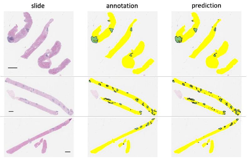
Figure 1: A coarse-level visualization of three representative core needle biopsy slides (left) alongside with LAs annotations provided by a renal pathologist (middle) and neural network prediction (right). Predictions with area less than 15,000 pixels are removed. The black horizontal bar indicates scale of 1 mm.

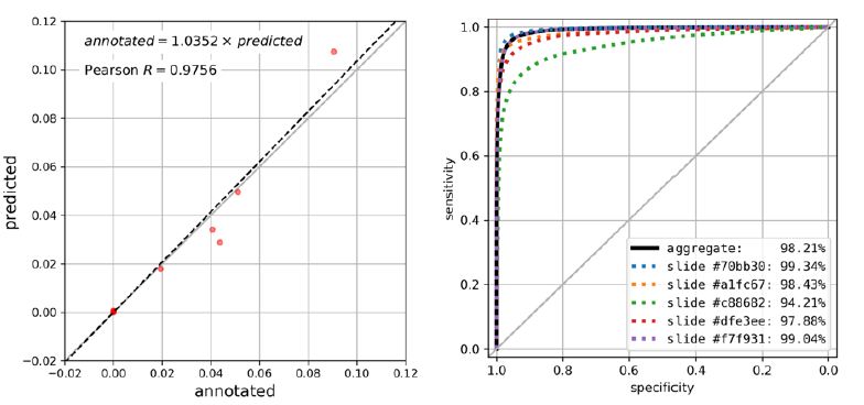
Figure 2: Performance metrics of the segmentation algorithm within the test set. A. Correlation plot of the area of LAs ROIs (as fraction of total tissue area) in annotations (x-axis) and predictions (y-axis), Pearson R of 0.9756 (p=1.5e-6). The regression line is shown in black dotted line, and regression equation is shown (p=5.874e-8). Note that 5 LA-free samples are densely clustered near the origin (0.0, 0.0). B. ROC curve for predicted probability of LAs-class pixels. ROC for all pixels aggregated across all samples is shown in black solid line (AUC=98.21, 95% confidence interval: 98.20-98.22% using DeLong method), and ROC for 5 individual LA-containing slides are shown in colored dotted lines. Diagonal grey line indicates ROC for random predictions.

Predicted LA areas were of wider range of sizes than annotated ones. Particularly, many small LAs were predicted compared to annotated ones. In order to further analyze the distribution of sizes and shapes of annotated and predicted LAs, we calculated areas and Polsby-Popper indices (PPI) characterizing the shape irregularity on the range from above 0 (highly irregular) to 1 (circular). The visualization of obtained metrics (Figure 3) reveals the presence of multiple small regular-shaped false-positive LAs predictions. An average area of the annotated LAs was 1,009,140 ± 134,419 pixels (64,339 ± 857μm²), while for predicted ones 301,600 ± 51,621 pixels (19,229 ± 3,291 μm²) in the test set. On the other hand, when only true positive predictions were matched with the annotations, the true positive areas were slightly larger than respective annotations, with regression equation: predicted area = 1.033 × annotated area (p<2.2e-16, Figure 3C). The shape irregularity was similar in both groups on average (PPI = 0.4397 ± 0.0225 for annotated and 0. 4418 ± 0.0098 for predicted, p=0.5376 in unpaired test). However, when only true positive predicted LAs were evaluated and paired with the annotations, the predicted LA regions have significantly less regular shape (PPI = 0.3165 ± 0.0180, p=2.557e-6 in paired Wilcoxon test), with regression equation (p<2.2e-16, Figure 3C):

Figure 3: Comparison of size and shapes of annotated and predicted ROIs. A. Distribution of area and Polsby-Popper index (PPI) for annotation ROIs (red triangles) and prediction ROIs (blue dots). True positive predicted ROIs are connected to respective annotation ROIs with yellow lines. Note that false negative ROIs (with no connecting lines) mostly have small area. B. Correlation between the PPI of predicted and annotated ROIs (Pearson R=0.4184, p=0.0012). C. Correlation between the area of predicted and annotated ROIs (Pearson R=0.7961, p=1.3e-13).

Predicted PPI = 0.6707 × Annotated PPI

As the minimal shape of annotated LAs was 33,782 pixels (2,153 μm²), with 5% percentile at 131,433 pixels (8,380 μm²), we sought to improve the performance of the segmentation by removing small predicted LA areas. To this end, we calibrated IoU performance as a function of low-pass area threshold within the validation set (Figure S3) and selected an optimal threshold for the area of predicted LAs that leads to maximal improvement in median IoU, at the value of 15,000 pixels (956 μm²). This thresholding improved the agreement between the counts of annotated and predicted LAs, thus reducing the mean absolute error from 13.0 to 6.57 LA regions per slide in validation set and from 14.1 to 6.7 LA regions per slide in the test set. At the same time, thresholding produced only a slight increase in IoU in LA-containing slides of the test set from 71.64% to 72.04%.

We show detailed visualization of correctly segmented, false negative, and false positive patches in Figure 4A, 4B, and 4C respectively. In most cases, the segmentation outline produced by the model had high overlap with the human annotation (IoU = 69.72 ± 6.24%), but contained more spatial detail than the annotation. Oftentimes, smaller areas of fibrotic tissue or other non-lymphoid tissue that were included by the annotator into LA segmentation were excluded by the model, thus leading to false negative predictions (Figure 4B). We saw that the model detected several smaller areas of lymphoid aggregates missed by the annotator initially (Figure 4C, columns 1&2). Dense nuclear areas of small atrophic tubules or tangentially cut tubules that expose multiple nuclei in the same plane were sometimes mis-classified as LAs, which is especially common for predictions with small area (under 33,000 pixels; Figure 4C, columns 3&4).

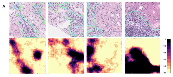
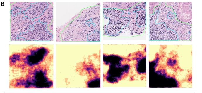
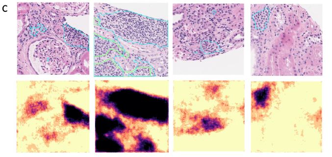
Figure 4: Segmentation of LAs in representative patches are shown with the original patch images and overlaid ground truth masks (green contour) and predictions (blue contour) in the top rows and segmentation probability heatmaps in the bottom rows. The IoU score, ground truth LA percentage, predicted LA percentage, slide ID, and patch coordinates are also displayed above each patch. A. Patches with good agreement between the annotation and prediction. B. Patches with false negative areas. C. Patches with false positive areas.

Discussion

Our study is the first to demonstrate that a deep convolutional neural network can accurately identify lymphoid aggregates and provide a quantitative measure of inflammation in digitized histological slides. It shows that inflammatory markers can be efficiently and robustly quantified automatically using DL, and thus shows potential of DL algorithms in improving efficiency and precision of renal pathology workup. Our model produces annotations of a higher spatial detail than present in typical manual annotations, while generally agreeing with the pathologist’s annotations, as seen in Figure 3A, and as indicated by a lower PPI index of true positive predicted LAs. Still the model produces numerous false positives of smaller size, that can be effectively removed by a low-pass area threshold filter. This shows that thorough expert-guided error analysis is necessary to keep medical DL algorithms unbiased, precise, and relevant to the problem at hand. On the other hand, our model detected areas of LAs initially missed by a pathologist (Figure4C, first column). This showcases the robustness and the power of the neural network model compared to human annotator, given sufficient amount of training data. Additionally, the increased speed at which LAs can be detected with our method will free up time for the already encumbered clinician to focus on other necessary tasks of the procedure.

Visualization tools used in this work to display density of LAs, such as in Figure 1, may be of potential use as a computer-aided decision support tool for pathologists and researchers investigating inflammatory processes in kidney allografts. As a next step, co-localization of lymphoid tissue with fibrotic and capsular tissue need to be learned as it is necessary for differential diagnosis of LA-associated conditions [18] similarly to systems developed to score inflammatory and fibrotic processes in lungs [25] and liver [26]. Furthermore, the scope of future work will need to expand to assigning and predicting Banff scores for various types of kidney pathologies [27]. We believe our model, fine-tuned with respective labels, would be able to accurately predict Banff lesions and provide basis for score estimation once we have adequate ground truth labels. Such an algorithm, when implemented as a part of a computer-aided diagnosis (CAD) system, could drastically speed up and simplify renal pathology analysis, as well as improve precision in clinics where specialized renal pathologists are not available.

Conclusions

Our study demonstrates that a deep convolutional neural network can accurately identify lymphoid aggregates in digitized histological slides of kidney. This study presents a first automatic DL-based approach for quantifying inflammation marks in allograft kidney, which can greatly improve precision and speed of assessment of allograft kidney biopsies when implemented as a part of computer-aided diagnosis system.

Funding

Research reported in this publication was supported by the National Institute of Health grants UH2CA203792, 1U01LM012675 (PI: DH), and U24AI118675 (PI: ZGL). AB is supported by a National Institute of General Medical Sciences training grant (5T32GM008440, PI: Judith Hellman). JHS is supported by T32 funding T32EB001631. The content is solely the responsibility of the authors and does not necessarily represent the official views of the National Institutes of Health.

Acknowledgment

In this section you can acknowledge any support given which is not covered by the author contribution or funding sections. This may include administrative and technical support, or donations in kind (e.g., materials used for experiments).

References

1. Jia Deng, Wei Dong, Socher R, Li-Jia Li, Kai Li, et al. (2009) ImageNet: A Large-Scale Hierarchical Image Database. In 2009 IEEE Conference on Computer Vision and Pattern Recognition 2009: 248-255.
2. Simonyan K, Zisserman A (2014) Very Deep Convolutional Networks for Large-Scale Image Recognition.
3. Esteva A, Robicquet A, Ramsundar B, Kuleshov V, DePristo M, et al. (2019) A Guide to Deep Learning in Healthcare. Nat Med 25: 24-29.
4. Topol EJ (2019) High-Performance Medicine: The Convergence of Human and Artificial Intelligence. Nat Med 25: 44-56.
5. Ching T, Himmelstein DS, Beaulieu-Jones BK, Kalinin AA, Do BT, et al. (2018) Opportunities and Obstacles for Deep Learning in Biology and Medicine. J R Soc Interface 15: 20170387. [crossref]
6. Ronneberger O, Fischer P, Brox T (2015) U-Net: Convolutional Networks for Biomedical Image Segmentation; Springer Cham. 234-241.
7. Badrinarayanan V, Kendall A, Cipolla R (2017) SegNet: A Deep Convolutional Encoder-Decoder Architecture for Image Segmentation. IEEE Trans. Pattern Anal Mach Intell 39: 2481-2495.
8. Litjens G, Bandi P, Ehteshami Bejnordi B, Geessink O, Balkenhol M, et al. (2018) 1399 H&E-Stained Sentinel Lymph Node Sections of Breast Cancer Patients: The CAMELYON Dataset. Gigascience 7: 65. [crossref]
9. Liu Y, Kohlberger T, Norouzi M, Dahl GE, Smith JL, et al. (2019) Artificial Intelligence–Based Breast Cancer Nodal Metastasis Detection: Insights Into the Black Box for Pathologists. Arch Pathol Lab Med 143: 859-868.
10. Campanella G, Hanna MG, Geneslaw L, Miraflor A, Werneck Krauss Silva et al. (2019) Clinical-Grade Computational Pathology Using Weakly Supervised Deep Learning on Whole Slide Images. Nat Med 25: 1301-1309. [crossref]
11. Meskó B, FDA Approvals For Smart Algorithms In Medicine In One Giant Infographic.
12. Ledbetter D, Ho L, Lemley KV (2017) Prediction of Kidney Function from Biopsy Images Using Convolutional Neural Networks.
13. Averitt AJ, Natarajan K (2018) Going Deep: The Role of Neural Networks for Renal Survival and Beyond. Kidney. Int Reports 3: 242-243. [crossref]
14. Marsh JN, Matlock MK, Kudose S, Liu TC, Stappenbeck TS, et al. (2018) Deep Learning Global Glomerulosclerosis in Transplant Kidney Frozen Sections. IEEE Trans Med Imaging 37: 2718-2728. [crossref]
15. Pei G, Zeng R, Han M, Liao P, Zhou X, et al. (2014) Renal Interstitial Infiltration and Tertiary Lymphoid Organ Neogenesis in IgA Nephropathy. Clin J Am Soc Nephrol 9: 255-264. [crossref]
16. Kayler LK, Lakkis FG, Morgan C, Basu A, Blisard D, et al. (2007) Acute Cellular Rejection with CD20-Positive Lymphoid Clusters in Kidney Transplant Patients Following Lymphocyte Depletion. Am J Transplant 7: 949-954. [crossref]
17. Girlanda R, Kleiner DE, Duan Z, Ford EAS, Wright E C, et al. (2008) Monocyte Infiltration and Kidney Allograft Dysfunction During Acute Rejection. Am J Transplant, 8: 600-607. [crossref]
18. Nadasdy T, Satoskar A, Nadasdy G (2017) Pathology of Renal Transplantation. In Silva’s Diagnostic Renal Pathology; Zhou, X. J. (Joseph), Laszik, Z. G., Nadasdy, T., D’Agati, V. D.
19. Goode A, Gilbert B, Harkes J, Jukic D, Satyanarayanan M () OpenSlide: A Vendor-Neutral Software Foundation for Digital Pathology. J Pathol Inform 2013, 4 (1), 27. [crossref]
20. Lituiev DS slideslicer: a toolbox for manipulation of digital pathology slides and annotations.
21. Balakrishna C, Dadashzadeh S, Soltaninejad S (2018) Automatic Detection of Lumen and Media in the IVUS Images Using U-Net with VGG16 Encoder.
22. Kingma DP, Ba J (2014) Adam: A Method for Stochastic Optimization.
23. Lituiev DS, Cha SJ, Chin A, Glicksberg BS, Bishara A, et al () Source Code for Automated Localization and Segmentation of Mononuclear Cell Aggregates in Kidney Histological Images Using Deep Learning.
24. Polsby DD, Popper R (1991) The Third Criterion: Compactness as a Procedural Safeguard Against Partisan Gerrymandering. Yale Law Policy Rev 9: 301-353.
25. Heinemann F, Birk G, Schoenberger T, Stierstorfer B (2018) Deep Neural Network Based Histological Scoring of Lung Fibrosis and Inflammation in the Mouse Model System. PLoS One 13: 202708. [crossref]
26. Heinemann F, Birk G, Stierstorfer B (2019) Deep Learning Enables Pathologist-like Scoring of NASH Models. Sci Rep, 9: 1-10.
27. Roufosse C, Simmonds N, Clahsen-van Groningen M, Haas M, Henriksen KJ, et al. (2018) 2018 Reference Guide to the Banff Classification of Renal Allograft Pathology. Transplantation 102: 1795-1814. [crossref]