DOI: 10.31038/GEMS.2026872

Abstract

The results indicate that tin enrichment is closely linked to processes occurring during the transition from supercritical to subcritical melt–fluid conditions. The Lorendian character of the distribution is consistent with critical phenomena, phase separation, and long-range correlation effects rather than conventional equilibrium partitioning. These findings support a model in which a substantial proportion of tin was introduced by mantle-derived supercritical fluids or melts, providing an alternative explanation for the exceptional enrichment observed in the Ehrenfriedersdorf deposit and related Variscan tin systems. Beyond its implications for the Ehrenfriedersdorf deposit, this study provides a new conceptual framework for understanding metal enrichment near critical melt–fluid transitions, with potential applications to the genesis of tin and other rare-metal deposits worldwide.

Keywords

Tin (Sn), Lorentzian distribution, Pseudo-Lorentzian distribution, Ehrenfriedersdorf tin deposit, Variscan tin deposits, Pegmatite, Pegmatitic quartz, Melt inclusions, Granitic melts, Ore-forming elements, Cassiterite (SnO₂) 

Introduction

Melt inclusions in pegmatitic quartz from the Variscan tin deposit Ehrenfriedersdorf, Erzgebirge, Germany, provide important information on the evolution of volatile-rich granitic melts and on the enrichment of ore-forming elements such as tin. During investigations of rehomogenized melt inclusions, different inclusions initially appeared to show variable proportions of glass and fluid. To evaluate these variations quantitatively, the water content of the inclusion systems was determined by Raman spectroscopy, and tin concentrations were measured by electron-microprobe techniques. This approach produced a large analytical data set in which water can be used as a common reference component for comparing the behavior of tin and other elements. A key requirement for this interpretation is the homogenization of melt inclusions at controlled temperatures and pressures. Previous experimental work demonstrated that melt inclusions from the Ehrenfriedersdorf pegmatite were trapped under different temperature-pressure conditions. Therefore, approximately 500 µm-thick doubly polished sections were prepared, and a new sample was used for each homogenization experiment. Experiments were carried out at constant pressure conditions of 1, 2, and 3 kbar and at temperature steps of 50°C between 500 and 750°C, with each step held for 20 hours. Additional intermediate temperature steps were later performed as controls. Further experimental details are given by Thomas et al. (2009) [1] in the electronic supplementary material. In the present contribution, tin is examined as a representative element because its distribution relative to water shows an unexpected and highly systematic pattern. Plotting Sn concentration against H₂O content reveals a Lorentzian-type distribution in projection, whereas the full interpretation requires consideration of the three-dimensional H₂O-temperature-Sn relationship. The aim of this study is therefore to describe the Lorentzian distribution of Sn, evaluate its geometric correction from the projected plane to the real solvus-curve path, and discuss the implications for element enrichment in the Ehrenfriedersdorf pegmatite system.

Sample Material

Pegmatite quartz from the Sauberg mine near Ehrenfriedersdorf, Erzgebirge, Germany, was used as the sample material. The investigated quartz contains melt inclusions that are suitable for reconstructing the composition and evolution of the pegmatitic melt. A concise description of the geological setting and sample background is given by Thomas (2026) [2], including the relevant references cited there. The data points used in the present study represent mean values calculated from at least ten paired measurements of H₂O content and Sn concentration. Where direct measurements were not available, selected values were obtained by interpolation to complete the distribution pattern.

Results

Figure 1 shows the generalized results of the tin and water determination in the coordinates X = H₂O in [%(g/g)], Y = temperature in °C, and Z = Sn concentration in ppm.We see from the three-dimensional diagram that Sn is related to the solvus curve (in the H₂O-temperature plane) and forms a three-dimensional shape, which shows as a projection to the parallel plane (H₂O-Sn) that goes through the critical point (25.9% H₂O at 720°C) of the solvus curve an even Lorentzian distribution curve.

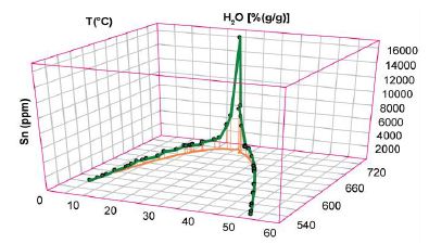
Figure 1: Distribution of Sn in the H₂O-T-Sn-room.

The computer (analyses with OriginPro 6.1) gives the following characteristic Lorentzian data (Table 1). Because the projected axes are Sn in ppm and H₂O in %, the projected area is approximately: ppm ∗ % H₂O. The Lorentzian curve for the projection onto the H₂O-Sn plane is shown in Figure 2.

Table 1: Results of the Lorentzian distribution (projection to the H₂O-Sn-plane).

Area	Center	Width	Offset	Height	R2
58852	25.7 % H2O	2.29 % H2O	582.2 ppm Sn	16345 ppm Sn	0.98356

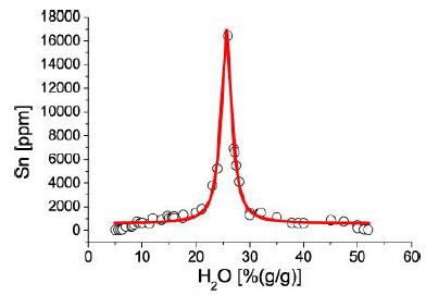
Figure 2: Lorentzian curve for Sn in the coordinates H₂O [%(g/g)] and Sn (ppm). The characteristic data are in Table 1.

Because this plot is only a projection into the H₂O-Sn plane, the area and width data are too small. To solve the area dilemma, we determine the arc segment of the solvus curve, for which the equation Y = 457.88726062 + 24.41440722*X – 0.67448344*X*X + 0.00446272*X*X*X is valid in the H₂O-T plane (H₂O = X, T = Y), between the points X₁ = 5.0 and X₂ = 52.0 and Y₁ = 563.7 and Y₂ = 531.2.

The arc-length integral is (see, for example, Thomson, 1956) [3]

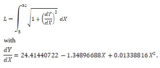
So

Also, the vertical change along the polynomial between the endpoints is approximately

Y (52) – Y (5) ≈ -32.5

but the curve first decreases strongly and then increases strongly, so the total traveled curve length is much larger than the straight-line endpoint distance.

Therefore:

L ≈ 433.74

The arc length 433.74 for the solvus curve is therefore, by division, the factor 433.74/32.5 ≈ 13.3. By this factor, the area of the room Lorentzian curve is greater than the projection (Table 2).

Table 2: Results of the corrected area of the room Lorentzian distribution.

Area	Center	Width	Offset	Height	R2
785,430	25.7 % H2O	30.6 % H2O	582.2 ppm Sn	16345 ppm Sn	0.98356

The area under the Lorentzian curve means the integrated amount represented by the peak.

In your case, the Lorentzian curve describes Sn concentration as a function of H₂O content. Therefore, the area is not just the maximum Sn value; it is the total Sn enrichment spread over the H₂O interval.

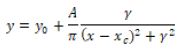
then:

•  is the background or offset,
• is the center of the peak,
• ϒ is the width parameter,
• A is the area of the Lorentzian peak above the background.

So the value Area = 58852 in Table 1 means:

the integrated Sn enrichment above the background in the projected H₂O–Sn plane.

Because the axes are H₂O in % and Sn in ppm, the projected area has the unit approximately:

ppm Sn ∗ %H₂O.

Thus,

58852 x 13.35 ≈ 7.86 x 10⁵

So the corrected area represents the integrated Sn enrichment along the real solvus-curve path, not only its 2D projection.

Using the same correction factor from your document, the real width for the room curve is:

With:

Projected width = 2.29 % H₂O

we get:

2.29 x 13.3458 = 30.56

So the real width is approximately: 30.6 % H₂O in the same corrected arc-length scale of the H₂O–T solvus curve. Applying the same arc-length correction factor used for the area, the projected Lorentzian width of 2.29% H₂O corresponds to a real room-curve width of approximately 30.6 units along the solvus curve (see Table 3).

Table 3: Results of the corrected area of the room Lorentzian distribution.

Area	Center	Width	Offset	Height	R2
785,674	25.7 % H2O	30.6 % H2O	582.2 ppm Sn	16345 ppm Sn	0.98356

An explanation of the data is in Table 4.

Table 4: Primary projected and corrected room-curve Lorentzian parameters.

Parameter	Primary projected value	Corrected room-curve value	Change
Area	58,852	≈ 785,674	Changes by the arc-length factor.
Center	25.7 % H2O	25.7 % H2O	No change in the H2O coordinate.
Width	2.29 % H2O	≈ 30.6 arc-length units	Changes if expressed along the real solvus curve.
Offset	582.2 ppm Sn	582.2 ppm Sn	No change; vertical Sn value.
Height	16,345 ppm Sn	16,345 ppm Sn	No change; vertical Sn value.
R2	0.98356	0.98356	No change in the fit quality.

Only the area and the width are transformed by the arc-length correction factor. The center, offset, height, and R² remain unchanged when they are reported in their original coordinates.

What Represents the Area?

The fitted area

A = 785 674 ppm Sn × % H₂O

and the integral is

where Sn is in ppm, and H₂O is expressed in percent. Thus, the area has mixed units and is not yet a mass.

Calculation of the Average Sn Concentration

The average concentration represented by the Lorentzian over the H₂O interval is

with

ΔH₂O = 30.6%.

The H₂O center remains 25.7% H₂O,

• The offset is 582.2 ppm Sn, and it represents the background Sn concentration or baseline level of the Lorentzian Because it is a vertical Z-value in ppm Sn, it is not affected by changing the horizontal coordinate from projected H₂O distance to real arc length.
• Raman-band positions were calibrated before and after each measurement series using the Si band of a semiconductor-grade single-crystal silicon chip. Based on 20 repeated measurements, run-to-run reproducibility was ± 0.2 cm⁻¹ for silicon (520.2 ± 2 cm⁻¹) in the range from 100 to 1450 cm⁻¹. As a second reference, a water-clear diamond crystal from Brazil was used. The first-order diamond line was measured at 1330.1 ± 0.6 cm⁻¹, with a FWHM of 5.1 ± 0.1 cm⁻¹ (see also Solin and Ramdas, 1970).
• The height also remains unchanged. The height value, 16345 ppm Sn,is a vertical concentration value in the Sn It describes how high the Lorentzian peak rises above the offset/background. Because the arc-length correction changes only the horizontal coordinate from projected H₂O distance to real distance along the solvus curve, it does not change vertical Sn values.

Discussion

We have shown that the simple Lorentzian function on projection to the H₂O-Sn plane is only a first approximation, because the room-curve of the Sn-distribution in the H₂O-T plane is significantly larger. From the arc-length integral, the total traveled curve length is much larger than the straight-line endpoint distance: L ≈ 433.74. As a result, the area and the width under the room curve significantly increase. That means that Sn enrichment in the pegmatites from Ehrenfriedersdorf is very large and incompatible with the enrichment of tin in granites. In Thomas (2026) [2], the Lorentzian data for 8 further elements are presented. The two Gaussian distributions (Zn, WO₃) in Table 1 are exceptions that must be tested. According to Hösel (1994) [4], the granites from Ehrenfriedersdorf contain, on average, 36.2 ± 17.7 ppm Sn and are typical Sn granites. Granites generally contain 3 ppm Sn [5]. That is an enrichment of about 12. The deposit contains many pegmatites and pegmatite-like bodies [6] see Figure D in it. So a rich Sn deposit as Ehrenfriedersdorf cannot be formed by further enrichment of Sn via hydrothermal processes. We would need a huge amount of water and a multistage enrichment process. This contribution shows evidence of a high-temperature source of tin and water. A large part of the Sn and water also comes with supercritical fluids (SCF) or supercritical melts (SCM) from mantle depths [7]. That fluid contains not only dissolved tin but also suspended crystals of orthorhombic cassiterite in high amounts, as demonstrated by Thomas (2024) [8].

Above, we have shown that the transition of a supercritical melt/ fluid (SCF, SCM) to a subcritical state occurs when temperature and/or pressure drop below the critical point. The following key things happen:

• Above the critical point, there is no sharp distinction between liquid and The material exists as a single supercritical phase.
• Crossing below the critical point restores the liquid-vapor phase A distinct liquid phase and single vapor phase can exist again.
• If the path crosses the coexistence curve, the fluid may separate into liquid and gas, often through nucleation and growth of bubbles or droplets.
• Near the critical point, properties such as diffusivity, viscosity, density, compressibility, and heat capacity change very rapidly.
• In many systems, the change is not always abrupt exactly at the critical point; supercritical fluids can pass through a region where they gradually change from liquid-like to gas-like This crossover concept is described as the Widom line.

From Figures 1 and 2 and Table 1 in Thomas (2026) [2], we know that a row of elements is Lorentzian distributed after a supercritical-to-subcritical transition, with enrichment factors from 1000 to 10000 at the center ~ equal to the critical point of the solvus curve. Such processes are usually critical-concentration mechanisms, not ordinary equilibrium partitioning.

Possible reasons include:

1. Critical-point density fluctuations:

Near the critical point, density fluctuations become extremely large. Certain trace elements may strongly prefer one local environment over another. As the system crosses into the subcritical regime, these fluctuations can “collapse” into separated phases, concentrating elements into narrow zones (boundary layers: see London, 2008) [9]. This can produce very sharp peaks, long tails resembling a Lorentzian distribution, and partition coefficients that exceed normal values.

2. Fluid-melt phase separation:

When a supercritical melt-fluid system unmixes, one phase may become highly enriched in incompatible elements, and the complementary phase becomes depleted. Element concentrations can increase by orders of magnitude if the enriched phase occupies only a tiny fraction of the volume (melt inclusion).

3. Spinodal decomposition (see Binder, 1987) [10]:

If the system enters a spinodal region rather than nucleating discrete droplets, composition waves form spontaneously, and peak concentrations may follow Lorentzian or Cauchy-like profiles because correlation lengths become very large near criticality.

4. Focusing by diffusion and advection:

During rapid decompression, the elements migrate toward fluid-rich channels; flow and diffusion can “focus” elements into narrow fronts. The resulting profile often has a sharp center and broad wings that are better fit by Lorentzian than Gaussian.

5. Nanoparticle or colloid transport:

Many metals, for example (Sn, Nb, Ta), can be transported as nanoclusters, colloids, or complex molecular processes with finite variance.

When the supercritical state breaks down, these species may precipitate into extremely small volumes (melt and fluid inclusions), generating apparent factors of 10000 or more.

Why specifically a Lorentzian distribution? A Gaussian profile usually indicates many independent random processes with a finite variance. A Lorentzian form often appears when correlation becomes long-ranged, critical phenomena dominate, rare large excursions control the distribution, and resonance or singular behavior occurs near a critical point [11].

Conclusions

Tin concentrations in melt inclusions from the Ehrenfriedersdorf deposit follow a pseudo-Lorentzian distribution in H₂O–T–Sn space, with enrichment closely associated with conditions near the supercritical–subcritical melt–fluid transition. Correcting for the geometry of the H₂O–temperature solvus reveals that conventional two-dimensional projections substantially underestimate the extent of Sn enrichment. The results suggest that critical phenomena played a major role in tin transport and accumulation and support a significant contribution of mantle-derived supercritical fluids or melts to ore formation. More broadly, this approach provides a new framework for investigating metal enrichment in tin and other rare-metal systems.

Acknowledgment

The author thanks Dr. Adolf Rericha (Falkensee, Germany) for the intense discussion on the Lorentzian distribution of elements.

References

1. Thomas R, Davidson P, Rhede D, Leh M (2009) The miarolitic pegmatites from Königshain: a contribution to understanding the genesis of Contrib Mineral Petrol 157: 505-523.
2. Thomas R (2026) Attempt to interpret the exceptional element enrichment and distribution in pegmatites related to the Variscan tin deposit at the example of Ehrenfriedersdorf, Geol Earth Mar Sci 8: 1-8.
3. Thompson SP (1956) Höhere Mathematik und doch verständlich. Pg: 238.
4. Hösel G (1994) Das Zinnerz-Lagerstättengebiet Ehrenfriedersdorf/ Freiberg. Pg: 195.
5. Rösler HJ, Lange H (1975) Geochenische VEB Deutscher Verlag für Grundstoffindustrie Leipzig. Pg: 700.
6. Schröcke H (1954) Zur Paragenese erzgebirgischer Zinnlagerstätten. Neues Jb Mineral. Abh 87: 33-109.
7. Thomas, R.; Davidson, P.; Rericha, A.; Recknagel, U (2023) Mineral inclusions in a crustal granite: Evidence for a novel transcrustal transport mechanism.Geosciences 13.
8. Thomas R (2024) The CaCl₂-to-rutile phase transition in SnO₂ from high to low pressure in Geol Earth Mar Sci 6: 1-4.
9. London D (2008) Pegmatites. The Canadian Mineralogist. Special Publication 10. Pg: 347.
10. Binder K (1987) Theory of first-order phase transition. Reports on Progress in Physics 50: 783-840.
11. Thomas R (1994) Estimation of the viscosity and the water content of silicate melts from melt inclusion EJM 6: 511-535.