Abstract
Rainfall precipitation on dumpsite dissolves organic and inorganic constituents, forming toxic chemicals thereby leaching into groundwater bodies resulting to generation of high biological oxygen demand (BOD), and thus contaminating the groundwater system and thereby resulting into the death of aquatic life. The impact is not limited to biodiversity as odour and vermin from dumpsites makes disease becomes an issue with other adverse concomitant health challenges. Effort to save the environment from further degradation necessitated this research. Geophysical and physico-chemical investigations were carried out across the dumpsite located at Kubwa, F.C.T. North-central Nigeria. The aim of the research is to delineate areas of possible contamination plume, its migration path and the vadose zones. For this purpose, Electrical resistivity tomography (ERT) data were acquired along eight traverses and results were inverted using RES2DINV Software likewise fifteen VES were equally acquired and results corroborate the ERT results. Water samples from boreholes, hand dug well and river channel were obtained and were analyzed. Distinct low resistivity zones that we adjudged to represent the contamination plumes were obtained from the ERT results. The water analysis revealed that the, total dissolved solid (TDS) were in the ranges of (2.30 x 101 to 8.20 x 101) μScm-1as against NSDWQ values of 1×10³ μScm-1. Biochemical oxygen demand (BOD), chemical oxygen demand (COD) and dissolved oxygen (DO), were in the ranges of 1-10, <2 to <98 and 0.01-0.12 mg/L respectively. The water samples also had detectable levels of Cu, Cd, Ni, Mn, Pb and Zn contents which are far below the permissible limits. The water samples microbiologically revealed presence of faecal contamination with bacteria pathogens such as Coliform, and Escherichia coli are above permissible limit, while the mould yeast and total aerobic are below the limit likewise. Ultimately, our findings showed that the investigated dumpsite constitutes a serious threat to groundwater body in the area. The efficacy of combined geophysical and physico-chemical approaches for groundwater contaminant studies has been demonstrated in this study.
Keywords
Leachate, Vadose zone, Contaminant Plumes, Physico-chemical, North Central Nigeria
Introduction
Dump materials are generated regularly as a result of human activities. The ferocity of these human activities has led to the growing amount of dump materials globally despite the level of worldwide advancement in technology. Ganiyu et al., (2016) [1] asserts that dumpsites serve as the ultimate recipient of municipal solid waste. Environments get Polluted when by-product of chemical substances infuse into natural habitats; and thus immensely alter nature’s ability to dispense these pollutants. Pollutants are materials which impose danger on the health of humans, causes discomfort and damages the environment. Sabahi et al., (2009) reports that air, soil, water, nuclear and oil pollution characterises major types of pollution. Huge amount of dumped materials from urban, municipal and industrial sectors are generated globally. According to Rukah and Al-Kofahi,(2001) [2], dumpsites have over many decades been used as harbours for varied dump materials. According to Vinai et al., (2015), dumpsites are either situated above the ground or located within quarries or pits. Poovarasan et al., (2018) throw more light on how physical, chemical and biological processes interact simultaneously to bring about the overall decomposition of wastes. Afangideh et al., (2015) described the end-products of all waste mechanisms as chemically laden leachates. Misra and Mani, (1991) attributed Leachates generated from dumpsites as sources of groundwater and soil pollutions. Leachate is characterised by high ion concentrations while the rock hosting them depicts low resistivity compared to surrounding rocks. Employing the geoelectrical techniques in mapping of the leachate has become necessary (Ganiyu et al., 2015) [3]. For example, Chen et al. (2020) [4] used a novel approach to assess the complexity of contaminant plume transportation in the aquifer based on Hausdorff Fractal Dimension. Furthermore, Chen, et al., (2019) [5]. Carried out the assessment of shallow groundwater contamination resulting from a municipal solid waste landfill-a case study in Lianyungang, China. Electrical Resistivity Tomography (ERT) studies on dumpsites were conducted by varied researchers to delineate leachate, contaminant plumes on the land and its effect on aquifer system. In this research work, the use of 2D resistivity Imaging and Vertical Electrical Sounding (VES) were employed to characterise the depth to the groundwater table, identify and characterise the extent of contaminant leachate plume and its migration flow paths at subsurface within and around dumpsite and the results were corroborated by physico-chemical analysis for robust research’s outcome.
Location Description and Geological Setting
The study area, F01 Kubwa refuse dumpsite (Figure 2.1) is located within Abuja F.C.T metropolis in Bwari Area Council and lies within longitudes E007°22.650¹n to E007°22.591¹ and latitudes N0910.079¹ to N0910.080¹ north-central Nigeria. It was in operation before 2011 and still in use till date (Figure 1).
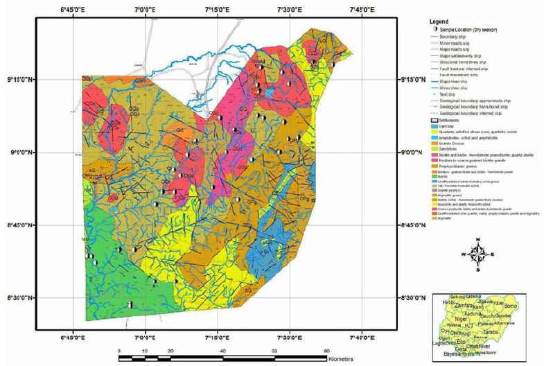
Figure 1: Geological Map of Abuja showing the Study Area (modified after NGSA 2004).
Geology of Abuja
Offodile (1992) described the geology and geomorphology of Abuja to have been underlain by crystalline basement rocks and it consists of rock types which contain different textures of granites, coarse to fine, consisting essentially of biotite, feldspars and quartz. In most cases, the rocks have weathered into reddish micaceous sandy-clay to clay materials capped by laterites [6]. Generally, only small amount of water can be obtained in the freshly unfractured bedrock below the weathered layers. Groundwater is found mainly in the variable weathered/transition zone which consist of fractures, joints and cracks of the crystalline basement [6]. Clark (1985) described fissure systems in Nigeria as rarely extends beyond 50m, as proven by the available drilling data. The local water table depth is controlled by textural and compositional changes within the regolith vertical profile and the bedrock topography according to David and Ofrey (1989) [7].
Methodology
Data Description, Acquisition and Processing
Electrical resistivity methods were adopted using Vertical Electrical Sounding (VES) and Electrical Resistivity Tomography (ERT) which are very much successful in delineating vertical variation and lateral of subsurface geology respectively. Comprehensive Geophysical studies using electrical resistivity were conducted with DC resistivity meter (Omega Allied). Omega Allied is an improved Digital resistivity meter with multi ingenious functional attributes inbuilt in its design and is known for its high quality data acquisition capability as well as for its field worthiness. It is a very close-packed, sophisticated and well grounded equipment, which is used for resistivity investigations. Omega Allied resistivity meter is made up of two units (i) Current unit (C unit), and (ii) Potential unit (P unit). This unit has the provision for measuring the potential difference across the potential electrode as well as the resistance values which provide direct display over digital panel metre. The current units provide the purpose of sending the required output of constant current, whereas the potential unit provides an accurate measurement and display. The depth of penetration is dependent on increase of electrode spacing, so that apparent resistivity measured at various depths is used to construct a vertical contoured section, displaying the resistivity contrast both laterally and vertically over the section. The 2D electrical resistivity pseudosection study was used in different locations in order to characterise the geology of various subsurface lithological, structural and hydrological conditions [8].
Wenner Arrangement
A simple method of determining the resistivity of the ground using four electrodes was discussed by Wenner (1916) otherwise called Horizontal Profiling (HP), when four electrodes are placed in a traverse line, and a known current is injected through the two extreme electrodes, the potential difference measured between the two inner electrodes gives a measure of the resistivity of the ground. The value of resistivity (ρ) is computed by the formula:
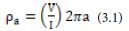
where, V is the potential in volts measured between the two inner electrodes, and I is the current in amperes passed into the ground, (a) is the distance between the successive electrodes and 2π, a constant. Since V/I = R, the resistance (Ω), the formula may be expressed as

In the above electrode arrangement, the two current electrodes are usually designated as C1 and C2, while the two inner electrodes, which pick up the potentials in the ground, are designated as P1 and P2, the potential electrodes or the measuring electrodes.
Schlumberger Array
In the Schlumberger array, letters A and B denoted the current electrodes while M and N represented potential electrodes. The distance between M and N may be represented by l, while the distance AB/2 is represented by L. During field layout, the current electrodes AB are placed as outer electrodes, while the two potential electrodes M and N as inner electrodes as shown in Figure 3.2. The Schlumberger array has major advantage in depth soundings in that, long current carrying cables may not be necessary. However, the ground consists of two or more layers with different resistivity contrast, and the electrode separation ‘a’ is less than the thickness of the first layer, then the measured resistivity value (Q1) will pertain to the first layer; on increasing the separation to, say (2a), thus the second layer having a different resistivity will make itself felt in the apparent resistivity measured. Therefore, by successively increasing the electrode separation about a central point, deeper depth of investigations of the earth may be measured. The apparent resistivity values obtained by expanding the electrode intervals are plotted against the respective electrode separations. In depth soundings using the Schlumberger array, the potential electrodes represented by M and N are kept fixed but the current electrodes A and B are moved farther away on either side, i.e., increasing the distance L, i.e. (AB/2) in successive steps and obtaining the resistivity values for a series of such increases for one setting of MN with interval of l. With this arrangement, deep investigation can be made in two or more settings, increasing also the spacing of the potential electrodes and then moving out the current electrodes. When the readings are completed for a particular spacing of the potential electrodes MN, the spacing of the latter is increased; whenever such a shift of MN is made, a duplicate reading is obtained while the current electrodes are still in the old setting this serve as to validate the integrity of the acquired data. Thereafter, only the current electrodes are shifted for the next set of observations. The resistivity curves obtained in depth soundings readily indicate the numbers of layers involved in the sounding depending on AB/2 spread length and number of geologic layer in the study area. But, if the ground under investigation is homogeneous and isotropic, the generated values of Q will be the true resistivity. Such ideal conditions rarely exist in the ground since earth is inhomogeneous, and the value of Q is usually affected by the variations in the lateral and vertical dimensions, particularly layered medium. Some various electrode arrays for the measurement of resistivity of the ground will be dealt with in this work (Figure 2).
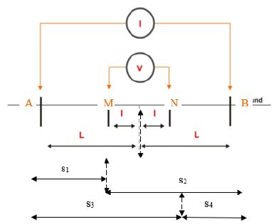
Figure 2: Schlumberger Array Layout.
Below equations below are generated from first principle.
Given that;
s1= (L – 1); s2= (L + 1); s3= (L + 1); s4= (L – 1)
in computing the geometric factor, we have ;
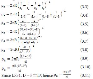
Physico-Chemical Analysis
A physico-chemical was carried out on the water sample from a borehole, an open hand dug well and river channel were considered.
Results and Discussion
Data Presentation and Interpretations
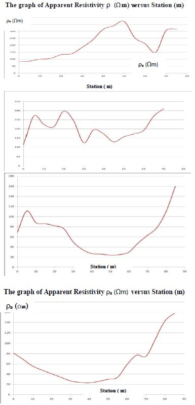
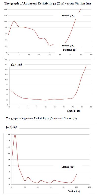
The Electrical Resistivity data using Horizontal Profiling (HP) were acquired along eight traverses and curves are presented in Figures 4.1-4.4 as 1D curves were generated using Microsoft excel showing characteristically low resistivity anomalies which coincide with dumpsite position while stations showing high anomalies are off the refuge positions, this was actually used as reconnaissance survey (Figure 3).
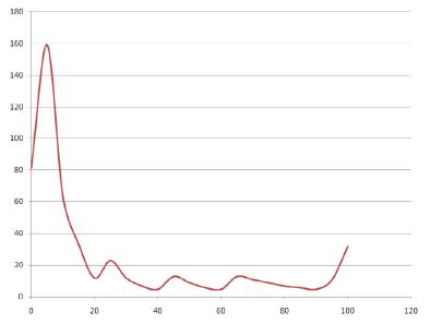
Figure 3: 1D Horizontal Profiling Curve for traverses 7 and 8.
Thereafter, 2D Electrical Resistivity Tomography (ERT) was employed along eight traverses, 2D Pseudosection models were generated using RES2DINV Software as shown in figures 4.9-4.16. Isoresistivity and Isopach maps in Figures 4.32-4.40 were equally generated from Vertical Electrical Sounding (VES) model curves in Figures 4.9-4.13. The data of wenner Array (HP) and VES model curve are presented. The VES model curves were generated from acquired data which were interpreted using qualitative and quantitative approach so as to classify the model curves according to the type of the curve, which are as follow; VES1, VES9, VES10, VES11 and VES12 depict KHA type curves: ρ1<ρ2>ρ3<ρ4>ρ5 VES2; ρ1>ρ2<ρ3>ρ4<ρ5 depicts HKH type curve, VES3and VES7: ρ1>ρ2<ρ3<ρ4>ρ5 depict HAK type curves, VES4, VES5 and VES8: ρ1<ρ2>ρ3<ρ4>ρ5 depict QHK type curves, VES6: ρ1<ρ2<ρ3>ρ4<ρ5 depicts AKA type curve, VES13 and VES14: ρ1<ρ2>ρ3<ρ4<ρ5 depict KHA type curves while VES15: ρ1<ρ2<ρ3>ρ4>ρ5.
Generated Isoresistivity maps, Isopach maps and Geoelectric section are presented as 2D images to further characterise subsurface geologic parameters. Subsequently geoelectric sections were as well produced as shown in figures 4.41-4.45. The anomalies observed on wenner array (HP) coincide with the area of low electrical resistivity as revealed by electrical tomography as indicated by 2D pseudosections (Figures 4-7).
Note: The high rms values recorded by the RES2DINV software is attributed to complexity of the dumpsite which pose challenge on electrode’s penetration into the ground through garbage materials as such several iterations were made and these seems to be the lowest rms values.
Interpreted Results of 2D Resistivity Pseudosection Models
The generated 2D pseudosections of the subsurface resistivity arrangement obtained from 2D inversion process are shown in Figures 4.9-4.16 were generated from acquired wenner data, these resistivity peudosections along traverses 1-8 reveals the distributional extend over the leachate plume across horizontal direction with distance of 7.5-90 m in the East-West direction which depicts resistivity reading of about 3.09 Ωm, which is attributed to presence of leachate plume summing up to 22 m depth below the earth surface and believed to have infiltrated into the groundwater table thereby polluting it, this was measured to be varying from 10-15 m as confirmed by the observable insitu samples from the borehole and open well due to joints, cracks and faulting system as result of deformation the subsurface rocks must have suffered, thus making the weathered and fractured basement below the basin-like structure leached easily. Infiltration of contaminant plumes within some of the traverse lines originate from the western end of the traverse where it infiltrates into subsurface. Figure 4.11 shows pseudosection model along third traverse with low resistivity contrasts below 17.6 Ωm attributed to leachate or contaminant plume’s migration which occur at horizontal distances 7.5-45.0 and 50-75.0 m along the traverse. Traverse 4 showing in Figure 4.12 indicates that the leachate, vadose zone and contaminant plumes region fall within the resistivity range of 10.5-120 Ωm and with the estimated depth of 1.25-7.6 m which overlaid fractured and fresh basement which have resistivity range of 125-6552 Ωm. Figure 4.13 and 4.14 showing psudosection model along traverse 5showingresistivity anomalies as low as 20 Ωm and below, this low resistivity values further indicate presence of leachate across the horizontal distance of 10.0–50.0 m and 55.0-82.0 m. The general resistivity values across the study area as shown in the 2D pseudosections were mostly less than 100.0 Ωm which coincides with the leachate, vadose zones and contaminant plumes regions at the surface. Traverse 6 pseudosection shows low resistivity ranges from 10.9-60 Ωm attributed to leachate portion along traverse 6, which covered the distance of 30-70 m which has depth of 9.26 m. Traverse 7 pseudosection model in Figure 4.14 shows a resistivity anomaly of 14.1-82.1 Ωm which is interpreted as leachate, vadose zone and contaminant plume region which covered distance of 7.5-95 m and the depth of 9 m deep. The traverses 7 and 8 where run north-south perpendicular to traverses 2-6 while traverse 1 was actually used as control since it was located some distance away from dumpsite. Contaminant plumes thus infiltrated weathered layer at depth 10-17 m with resistivity values ranging from 12-100 Ωm showing characteristics of possible infiltration of leachate thereby contaminating the groundwater at greater depth at the under study dumpsite. Relatively low resistivity anomaly of resistivity values 3.05-12.3 Ωm to a depth of about 7.26 m occurs at the near surface indicating presence of sandy-clay mixed with indestructible garbage. The resistivity displayed by the pseudosection models across traverses 1-6 are shown in Figures 4.9-4.14. From these 2D sections, low resistivity inconsistencies were observed across traverse 1-8 within the study area. This observed low resistivity anomalies along the major traverses showed characteristics of uniform movement of contaminant plumes from western to eastern direction and downward infiltration up to about 17 m depth at subsurface. This is underlain by fractured basement rock with resistivity values ranging between 100 and 550 Ωm. The 2D resistivity inversion model sections of the subsurface resistivity distribution derived from 2D inversion models depict that the study area structurally controlled considering 2D resistivity inversion models of traverses 3-8 presented in figures 4.11-4.16 showed major resistivity low which could be attributed to possible fractured zones.
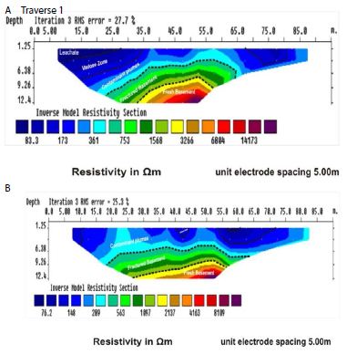
Figure 4(a & b): 2D Resistivity Pseudosection Model for traverses 1 and 2.
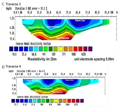
Figure 5(c &d): 2D Resistivity Pseudosection Model for traverses 3 and 4.
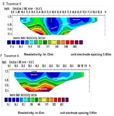
Figure 6(e & f): 2D Resistivity Pseudosection Model for traverses 5 and 6.
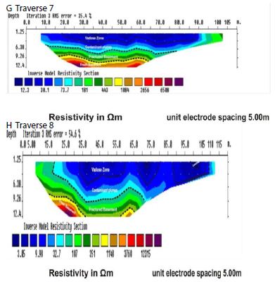
Figure 7(g &h): 2D Resistivity Pseudosection Model for traverses 7 and 8.
The resistivity pseudosection results along traverse 7 and 8 depicts general trend of uniform spreading of the contaminant plume from horizontal distance of 8-82 m along the North-South direction showing resistivity values 10 Ωm and below, this is an indication of leachate plume building up to the depth of about 12.4 m at the subsurface. It is obviously showing the 2D pseudosections that leachate plume formation migrate uniformly along both horizontal and vertical directions within the dumpsite. The low resistivity contrast of the upper stratum indicates that the underlying layer has higher resistivity values ranging between 140 and 300 Ωm indicating weathered or fractured basement across traverse1-8 in the study area. The central part of traverses showing in figures 4.11-4.16 the 2D pseudosection models with characteristics of low resistivity anomaly were observed between the positions 10-60 m with resistivity values ranges between 14 and 60 Ωm, this is an indicative of contaminant plumes at depth of about 12.4 m below the surface. The subsurface low resistivity was not quite obvious between 7.5 and 22 m along the traverse 1. A relatively high resistivity anomalies with resistivity values between 100 and 1097 Ωm attributed to fractured basements were observed at depth above 12.4m. The last layer of the pseudosections reveals an undulating fresh basement across traverses 1-8 with relatively high resistivity values between 1097 and 14173 Ωm. The 2D pseudosection models of traverses3-8in figures 4.11-4.16 show two major low resistivity anomalies situated at 7.5-90 m in the eastern and central portion across the traverses respectively with resistivity values below 50 Ωm, which further characterize the dumpsite into leachate, vadose zones and contaminant plume (Figures 8-12 and Tabes 1-15).
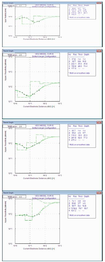
Figure 8: VES1-3 Model Curve along traverses 1.
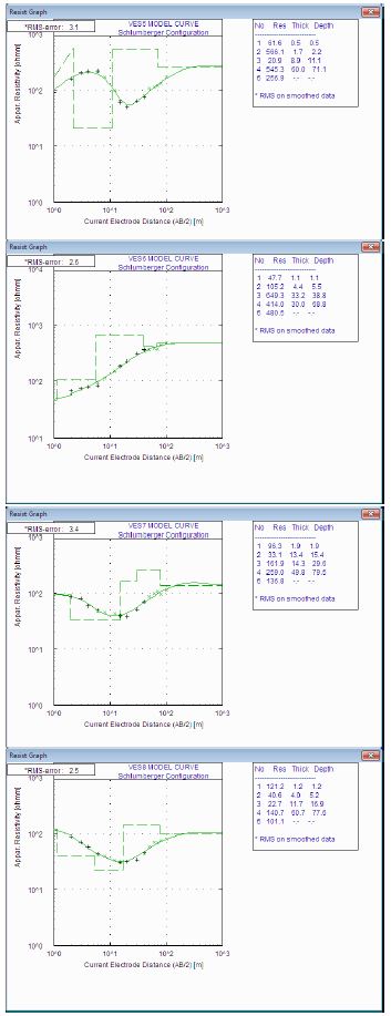
Figure 9: VES4-6 Model Curves along traverses 2.
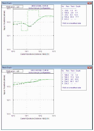
Figure 10: VES7-9 Model Curves along traverse 3.
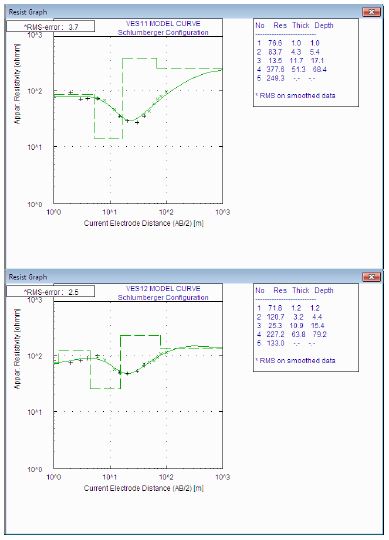
Figure 11: VES10-12 Model Curve along traverse 4.
Isoresistivity and Isopach Maps of the First to Fourth Layers
The Isoresistivity and Isopach maps of the first layer to fourth layer generated from VES1-VES 15 interpreted data were presented in Figure 4.32-4.40. The Isopach map for layer 1 indicates thickness ranging from 0.5-1.9 m. The map shows thickness in the south-Eastern part of the study area with thickness up to 1.3m which shows characteristics of leachate, while the Isoresistivity map indicates a resistivity range of 30.0-240.0 Ωm. The isoresistivity map and Isopach maps of layer 2 depict 20-580 Ωm and 1.5-13.5 m respectively which show an average thickness of about 6m which could be attributed to vadose zone. The third layer indicates the thickest thickness 6.0-54.0 m and its Isoresistivity map ranges from 50-950 Ωm. These three layers consist of resistivity low as indicated in 2D maps of both isoresistivity and isopach which thus attributed the contaminant leachate, vadose zone and plume zone respectively within the study area. The higher resistivity values were identified towards the southwestern, southeastern and central parts of the area up to 1300 Ωm and lowest resistivity values were identified in the Northern part of the study area ≤100 Ωm with the thickness values range from 25-95 m. This layer depicts competent geologic materials which is referred to as fractured basement layer which is underlain by fresh basement with the resistivity ranges from 100-800 Ωm. Very low resistivity suggests sandy-clay materials. Thus, water saturated materials, often infiltrated by leachate. The depth of the aquifer units range between 20 m and 30 m in the area which probably have been contaminated as a result of hydraulic communication through joints, crack and faulting which was further proved by the physico-chemical and microbiological analysis results. The Geochemical analysis further corroborate the geophysical interpretation by given insight to dissolve trace elements presence in water samples from borehole, hand dug well as well as stream water sample (Figures 13 and 14).
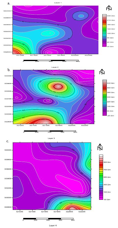
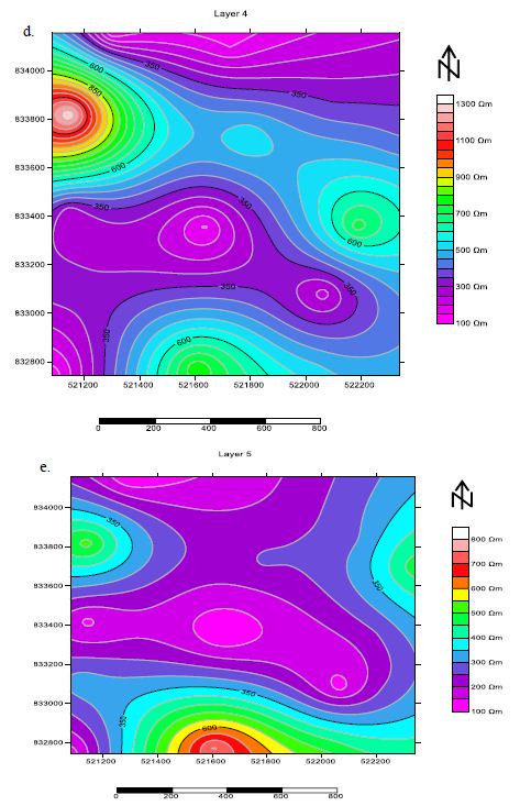
Figure 13(a-e): Isoresistivity map for layer 1-5.
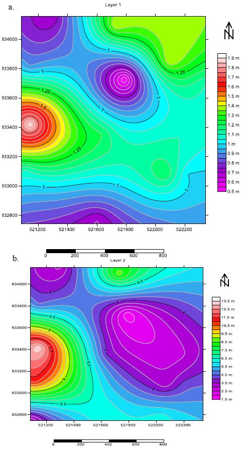
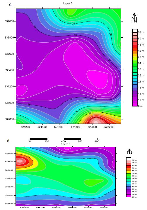
Figure 14(a-d): Showing Isopach map for layer 1-4.
2D Geoelectric Sections of the First to Fifth Layers
The interpreted VES1-VES15 results from Table 1-15 were equally used to generate 2D geo-electric sections (Figures 4.32-4.37). The geo-electric sections revealed five geo-electric sections of subsurface images based on layers comprising the lateritic topsoil(resistivity varies from 32.7-235.3Ωm and thickness range from 0.5 to 1.9 m); second layer laterite horizon (resistivity varies from 40.6 to 566.1 Ωm and thickness range from 2.2 to 11.3m); third layer sandy – clay ( resistivity varies from 12.5-36.7 Ωm and thickness range from 8.0 to 34.8 m; fourth layer fractured basement (resistivity varies from 111.6-1312.2 Ωm and thickness range from 28.9 to 79.7) m the resistivity value of the fifth layer fresh basement range from 101.1-759.1Ωm (Figures 15-17).
Table 1: VES1 interpreted result.
|
S/N |
Resistivity(Wm) | Thickness (m) | Depth (m) |
Lithological equivalence |
|
1 |
36.6 | 0.7 |
0.7 |
Lateritic topsoil |
|
2 |
131.6 | 2.2 |
2.9 |
Laterite |
|
3 |
16.4 | 14.1 |
17.0 |
Sandy-clay |
|
4 |
111.6 | 29.1 |
46.1 |
Fractured basement |
|
5 |
102.0 | ……….. |
……. |
Fresh basement |
Table 2: VES2 interpreted result.
|
S/N |
Resistivity(Wm) | Thickness (m) | Depth (m) |
Lithological equivalence |
|
1 |
57.8 | 1.4 |
1.4 |
Lateritic topsoil |
|
2 |
18.7 | 8.8 |
10.2 |
Sandy-clay |
|
3 |
222.1 | 35.6 |
45.8 |
Fractured Basement |
|
4 |
150.8 | 28.9 |
74.4 |
Fractured basement |
|
5 |
177.9 | ……….. |
………. |
Fresh basement |
Table 3: VES3 interpreted result.
|
S/N |
Resistivity (Wm) | Thickness (m) | Depth (m) |
Lithological equivalence |
|
1 |
95.7 | 1.4 |
1.4 |
Lateritic topsoil |
|
2 |
35.2 | 4.3 |
6.7 |
Sandy-clay |
|
3 |
110.2 | 19.6 |
25.3 |
Fractured Basement |
|
4 |
361.8 | 52.0 |
77.3 |
Fractured basement |
|
5 |
275.4 | ……….. |
…… |
Fresh basement |
Table 4: VES4 interpreted result.
|
S/N |
Resistivity(Wm) | Thickness (m) | Depth (m) |
Lithological equivalence |
|
1 |
74.1 | 0.9 |
0.9 |
Lateritic topsoil |
|
2 |
90.8 | 3.7 |
4.5 |
Laterite |
|
3 |
36.7 | 9.4 |
14.0 |
Sandy-clay |
|
4 |
1312.2 | 79.7 |
93.7 |
Fractured basement |
|
5 |
521.2 | ……….. |
………. |
Fresh basement |
Table 5: VES5 interpreted result.
|
S/N |
Resistivity(Wm) | Thickness (m) | Depth (m) |
Lithological equivalence |
|
1 |
61.6 | 0.5 |
0.5 |
Lateritic topsoil |
|
2 |
566.1 | 1.7 |
2.2 |
Laterite |
|
3 |
20.9 | 8.9 |
11.1 |
Sandy-clay |
|
4 |
545.3 | 60.0 |
71.1 |
Fractured basement |
|
5 |
256.9 | ……….. |
……. |
Fresh basement |
Table 6: VES6 interpreted result.
|
S/N |
Resistivity(Wm) | Thickness (m) | Depth (m) |
Lithological equivalence |
|
1 |
47.7 | 1.1 |
1.1 |
Lateritic topsoil |
|
2 |
105.2 | 4.4 |
5.5 |
Laterite |
|
3 |
649.3 | 33.2 |
38.8 |
Fractured Basement |
|
4 |
414.0 | 30.0 |
68.8 |
Fractured basement |
|
5 |
480.5 | ……….. |
……. |
Fresh basement |
Table 7: VES7 interpreted result.
|
S/N |
Resistivity(Wm) | Thickness (m) | Depth (m) |
Lithological equivalence |
|
1 |
96.3 | 1.9 |
1.9 |
Lateritic topsoil |
|
2 |
33.1 | 13.4 |
15.4 |
Sandy-clay |
|
3 |
161.9 | 14.3 |
29.6 |
Saprolite/weathered basement |
|
4 |
259.0 | 49.8 |
79.5 |
Fractured basement |
|
5 |
136.8 | ……….. |
……. |
Fresh basement |
Table 8: VES8 interpreted result.
|
S/N |
Resistivity (Wm) | Thickness (m) | Depth (m) |
Lithological equivalence |
|
1 |
121.2 | 1.2 |
1.2 |
Lateritic topsoil |
|
2 |
40.6 | 4.0 |
5.2 |
Laterite |
|
3 |
22.7 | 11.7 |
16.9 |
Sandy-clay |
|
4 |
140.7 | 60.7 |
77.6 |
Fractured basement |
|
5 |
101.1 | ……….. |
…… |
Fresh basement |
Table 9: VES9 interpreted result.
|
S/N |
Resistivity(Wm) | Thickness (m) | Depth (m) |
Lithological equivalence |
|
1 |
63.8 | 1.1 |
1.1 |
Lateritic topsoil |
|
2 |
109.8 | 2.9 |
4.1 |
Laterite |
|
3 |
23.2 | 8.0 |
12.0 |
Sandy-clay |
|
4 |
726.4 | 65.6 |
77.6 |
Fractured basement |
|
5 |
243.2 | ……….. |
…… |
Fresh basement |
Table 10: VES10 interpreted result.
|
S/N |
Resistivity(Wm) | Thickness (m) | Depth (m) |
Lithological equivalence |
|
1 |
128.2 | 1.1 |
1.1 |
Lateritic topsoil |
|
2 |
199.3 | 11.3 |
12.5 |
Laterite |
|
3 |
198.0 | 8.2 |
20.6 |
Sandy-clay |
|
4 |
334.5 | 60.1 |
80.7 |
Fractured basement |
|
5 |
330.3 | ……….. |
…… |
Fresh basement |
Table 11: VES11 interpreted result.
|
S/N |
Resistivity (Wm) | Thickness (m) | Depth (m) |
Lithological equivalence |
|
1 |
76.6 | 1.0 |
1.0 |
Lateritic topsoil |
|
2 |
83.7 | 4.3 |
5.4 |
Laterite |
|
3 |
12.5 | 11.7 |
17.1 |
Sandy-clay |
|
4 |
377.6 | 51.3 |
68.4 |
Fractured basement |
|
5 |
249.3 | ……….. |
………. |
Fresh basement |
Table 12: VES12 interpreted result.
|
S/N |
Resistivity (Wm) | Thickness (m) | Depth (m) |
Lithological equivalence |
|
1 |
71.8 | 1.2 |
1.2 |
Lateritic topsoil |
|
2 |
120.7 | 3.2 |
4.4 |
Laterite |
|
3 |
25.3 | 10.7 |
15.4 |
Sandy-clay |
|
4 |
227.2 | 63.8 |
79.2 |
Fractured basement |
|
5 |
133.0 | ……….. |
……. |
Fresh basement |
Table 13: VES13 interpreted result.
|
S/N |
Resistivity(Wm) | Thickness (m) | Depth (m) |
Lithological equivalence |
|
1 |
235.3 | 0.8 |
0.8 |
Lateritic topsoil |
|
2 |
370.7 | 2.4 |
3.2 |
Laterite |
|
3 |
82.8 | 34.8 |
37.9 |
Sandy-clay/weathered basement |
|
4 |
116.3 | 36.2 |
74.1 |
Fractured basement |
|
5 |
118.0 | ……….. |
……. |
Fresh basement |
Table 14: VES14 interpreted result.
|
S/N |
Resistivity(Wm) | Thickness (m) | Depth (m) |
Lithological equivalence |
|
1 |
32.7 | 0.7 |
0.7 |
Lateritic topsoil |
|
2 |
571.6 | 6.4 |
7.1 |
Laterite |
|
3 |
154.5 | 18.2 |
25.3 |
Sandy-clay/Weathered basement |
|
4 |
796.9 | 39.2 |
64.5 |
Fractured basement |
|
5 |
759.1 | ……….. |
………. |
Fresh basement |
Table 15: VES 15 interpreted result.
|
S/N |
Resistivity(Wm) | Thickness (m) | Depth (m) |
Lithological equivalence |
|
1 |
78.6 | 0.9 |
0.9 |
Lateritic topsoil |
|
2 |
24.6 | 6.3 |
7.2 |
Sandy-clay |
|
3 |
1069.0 | 53.6 |
60.9 |
Fractured basement |
|
4 |
514.4 | 38.9 |
100.8 |
Fractured basement |
|
5 |
484.8 | ………. |
……. |
Fresh basement |
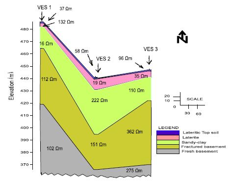
Figure 15: Showing Geoelectric section along traverse 1.
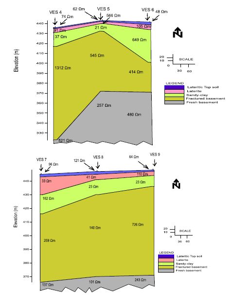
Figure 16: Showing Geoelectric section along traverse 2 and 3.
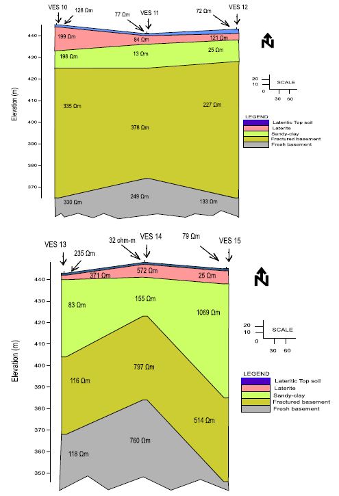
Figure 17: Showing Geoelectric section along traverse 4 and 5.
Evaluation of Leachate on Groundwater Quality
Leachate is generated by the degradation of waste and the process of water coming into contact with and infiltrate through, waste materials [9]. Generated Leachate varies in its chemical constituents from dumpsite to dumpsite and also depends upon numerous factors such as waste composition, ambient temperatures and rainfall or precipitation characteristics. However, leachate may have increased concentrations of numerous organic and inorganic pollutants [10]. The following metals were equally analyed in this study which include cadmium (Cd), Chromium, iron (Fe), lead, Magnesium Mg) and (Pb). Generally, the concentrations of the metals (except Fe which ranges from 0.01-0.20 mg L⁻¹) were not detected at F01 Kubwa leachate. This is due to the fact that the landfills received mainly municipal solid waste and very low quantities of industrial waste including batteries, radios and other Electronic gadgets.
Analysis of the Effects of Leachate and Contaminant Plume on Groundwater Quality
The importance of determining adverse effects of various elements that reach groundwater through leachate upon human health has gained momentum during the past decade [9]. The different approaches presume that, a sound scientific data base exists to defining the maximum exposure levels for a specific chemical compound. In this study, the pollutant indicators results obtained from groundwater monitoring program of the observation borehole, open well and River channel around F01 Kubwa dumpsite was used to study the effects of leachate formed from dumpsite on groundwater system.
Interpreted Results of Water Samples from Borehole, Open Well and River Channel
The low Electrical Conductivity (EC) measurements values in the water samples near the dumpsites give indications of its effect on groundwater. The EC values at the dump sites were below the NSDWQ suggested levels (1000 μs cm⁻¹). According to Abu Rukah and Al-Kofahi, (2001) [2] water conductivity within 1000 μs cm⁻¹ is suitable for irrigation purpose. It is important to note that the electric conductivity of the groundwater under F01 Kubwa dumpsite is lower of water conductivity of (230-460 μs cm⁻¹) as shown in tables. The followings are major anions tested in this study which are Chloride (Cl⁻), Nitrate (NO3-2) and sulphate (SO4-2).Faust and Aly, (1983) illustrated that Chloride in reasonable concentration is not harmful, but it aids corrosion in concentrations above 250 mg L⁻¹, while about 400 mg L⁻¹ of Chloride causes a salty taste in water Tamer et al (2011) [9]. Chloride concentration was measured and the range is not acceptable according to those permissible by NIGERIA INDUSTRIAL STANDARD (NIS)” 977: 2017 for potable water as shown in table 4.16-4.20 respectively. The geochemical investigation concluded that the water samples are physico-chemically and microbiologically unsatisfactory base on the parameters as shown in the tables 4.16-4.21 which were generated from physico-chemical analysis shown in appendix C, which thus corroborate the geophysical findings (Tables 16-21).
Table 16: Physico-chemical analysis for borehole sample.
|
Physio-Chemical parameter |
Result of Sample |
NSDWQ |
| PH |
7.10 |
6.5 – 8.5 |
| Conductivity, μs cm-1 |
2.30 x 10² |
1 x 10³ |
| Total alkalinity, mg L-1 |
57 |
100 |
| P. Alkalinity, mg L-1 |
Nill |
100 |
| M. Alkalinity, mg L-1 |
57 |
100 |
| TDS, ppm |
115 |
500 |
| Free Chlorine |
Nill |
0.1 |
| Freely dissolved CO2, mg L-1 |
21 |
50 |
| Total Chloride, mg L-1 |
18 |
200 |
| Total Hardness, mg L-1 |
73 |
150 |
| Nitrite, mg L-1 |
0.00 |
0.02 |
| Nitrate, mg L-1 |
0.00 |
10 |
| Lead, mg L-1 |
0.00 |
0.01 |
| Cadmium, mg L-1 |
0.00 |
0.003 |
| Chromium, mg L-1 |
0.00 |
0.01 |
| Arsenic, mg L-1 |
0.00 |
0.01 |
| BOD, mg L-1 |
1 |
1-3 |
| COD, mg L-1 |
<2 |
– |
| TOC, mg L-1 |
0.01 |
0.5 |
| Iron,mg L-1 |
0.01 |
0.3 |
| Sulphate, mg L-1 |
0 |
200 |
Table 17: Microbiological analysis for borehole sample.
|
TEST |
COUNT |
LIMIT |
| Total aerobic bacteria plate count cfu/ml |
1.1 x 101 |
1 x 10² |
| Mould/Yeast, cfu/ml |
2.0 x 100 |
1 x 10² |
| Coliform, MPN/100 ml |
11 |
0 |
| E. coli, MPN/100 ml |
0 |
0 |
Table 18: Physico-chemical analysis for open well.
|
Physio-Chemical parameter |
Result of Sample |
NSDWQ |
| PH |
7.40 |
6.5 – 8.5 |
| Conductivity, μs cm-1 |
8.20 x 10² |
1 x 10³ |
| Total alkalinity, mg L-1 |
87 |
100 |
| P. Alkalinity, mg L-1 |
Nill |
100 |
| M. Alkalinity, mg L-1 |
87 |
100 |
| TDS, ppm |
410 |
500 |
| Free Chlorine |
Nill |
0.1 |
| Freely dissolved CO2, mg L-1 |
35 |
50 |
| Total Chloride, mg L-1 |
18 |
200 |
| Total Hardness, mg L-1 |
89 |
150 |
| Nitrite, mg L-1 |
0.01 |
0.02 |
| Nitrate, mg L-1 |
0.09 |
10 |
| Lead, mg L-1 |
0.00 |
0.01 |
| Cadmium, mg L-1 |
0.00 |
0.003 |
| Chromium, mg L-1 |
0.00 |
0.01 |
| Arsenic, mg L-1 |
0.00 |
0.01 |
| BOD, mg L-1 |
3 |
1-3 |
| COD, mg L-1 |
<8 |
– |
| TOC, mg L-1 |
0.12 |
0.5 |
| Iron,mg L-1 |
0.09 |
0.3 |
| Sulphate, mg L-1 |
0 |
200 |
Table 19: Microbiological analysis for open well.
|
TEST |
COUNT |
LIMIT |
| Total aerobic bacteria plate count cfu/ml |
8.1 x 101 |
1 x 10² |
| Mould/Yeast, cfu/ml |
2.1 x 101 |
1 x 10² |
| Coliform, MPN/100 ml |
240 |
0 |
| E. coli, MPN/100 ml |
21 |
0 |
Table 20: Physico-chemical analysis for river channel.
|
Physio-Chemical parameter |
Result of Sample |
NSDWQ |
| PH |
7.20 |
6.5 – 8.5 |
| Conductivity, μs cm-1 |
4.60 x 10² |
1 x 10³ |
| Total alkalinity, mg L-1 |
65 |
100 |
| P. Alkalinity, mg L-1 |
Nill |
100 |
| M. Alkalinity, mg L-1 |
65 |
100 |
| TDS, ppm |
230 |
500 |
| Free Chlorine |
Nill |
0.1 |
| Freely dissolved CO2, mg L-1 |
21 |
50 |
| Total Chloride, mg L-1 |
14 |
200 |
| Total Hardness, mg L-1 |
64 |
150 |
| Nitrite, mg L-1 |
0.02 |
0.02 |
| Nitrate, mg L-1 |
1.00 |
10 |
| Lead, mg L-1 |
0.00 |
0.01 |
| Cadmium, mg L-1 |
0.00 |
0.003 |
| Chromium, mg L-1 |
0.00 |
0.01 |
| Arsenic, mg L-1 |
0.00 |
0.01 |
| BOD, mg L-1 |
10 |
1-3 |
| COD, mg L-1 |
<98 |
– |
| TOC, mg L-1 |
0.01 |
0.5 |
| Iron,mg L-1 |
0.20 |
0.3 |
| Sulphate, mg L-1 |
0 |
200 |
Table 21: Microbiological analysis for river channel.
|
TEST |
COUNT |
LIMIT |
| Total aerobic bacteria plate count cfu/ml |
4.3 x 101 |
1 x 10² |
| Mould/Yeast, cfu/ml |
1.1 x 101 |
1 x 10² |
| Coliform, MPN/100 ml |
53 |
0 |
| E. coli, MPN/100 ml |
13 |
0 |
Conclusion
Electrical resistivity tomography (ERT) method and Physicochemical analysis approach were employed to investigate active dumpsite at F01, Kubwa Extension, Abuja F.C.T North-central Nigeria. The 2D resistivity image of subsurface structure delineated the contaminant plume, leachate and thus further characterise the dumpsite based on subsurface resistivity apportionment of vadose zones, contaminant plumes and the hydrogeological conditions underneath the study area. 1D curves were interpreted both qualitatively and quantitatively to detect leachate, vadose zones and possible extent of pollution infiltrating groundwater system. The results of fifteen VES curves further classified the curve types of study area into five layers as shown in the model curves in figures 4.17-4.31 and tables 4.1-4.15 which classified as follows: VES1, VES9, VES10, VES11 and VES12 depict KHA type curves: ρ1<ρ2>ρ3<ρ4>ρ5 VES2; ρ1>ρ2<ρ3>ρ4<ρ5 depicts HKH type curve, VES3 and VES7: ρ1>ρ2<ρ3<ρ4>ρ5 depict HAK type curves, VES4, VES5 and VES8: ρ1<ρ2>ρ3<ρ4>ρ5 depict QHK type curves, VES6: ρ1<ρ2<ρ3>ρ4<ρ5 depicts AKA type curve, VES13 and VES14: ρ1<ρ2>ρ3<ρ4<ρ5 depict KHA type curves while VES15: ρ1>ρ2<ρ3>ρ4>ρ5.
Isoresistivity maps, Isopachmaps and Geoelectric section were equally generated from VES1-15 and presented as 2D images to further characterise subsurface geologic parameters. The anomalies observed on wenner array (HP) coincide with the area of low electrical resistivity as revealed by electrical resistivity tomography (ERT) as indicated by 2D pseudosection models; the results further conclude that the study area is structurally controlled.
Physico-chemical analysis revealed possible elemental contaminants within groundwater system. Leachate from dumpsite is a major pollutant contaminating groundwater body. The situation is currently bad and is expected to become worse in the near future Tamer et al (2011) [9]. The analysed results of physico-chemical parameters of the water samples corroborate the georesistivity interpretations, thus the physico-chemical results revealed that analysed sample fall below NSDWQ (2007) [11-43]. as shown in appendix C specification limits for portable water purpose. Therefore, effect of leachate infiltrating the dumpsite’s surrounding or agricultural run-off and fertilizer application might have raised ion concentrations of some parameters on open well, and river channel respectively. There is possible adulteration of shallow groundwater body around the central region of the dumpsite as results of strong manifestation of leachate movement and degree of infiltrating soil around the dumpsite as a result of possible structural geologic deformations the study area might have suffered.
Analyses of samples of F01 Kubwa showed that the total dissolved solid (TDS) were in the ranges of (2.30 x 10¹-8.20 x 10¹) μScm⁻¹ as against NSDWQ values of 1×10³μScm⁻¹; Total alkalinity, TDS, freely dissolved CO2, total chloride, total hardness (TH) and sulphate were 57-87, 115-410, 21-35, 14-18, 64-89mg/Land 0 respectively.
Biochemical oxygen demand (BOD), chemical oxygen demand (COD) and dissolved oxygen (DO), were in the ranges of 1-10, <2-<98 and 0.01-0.12mgL⁻¹ respectively. The water samples had detectable levels of Cu, Cd, Ni, Mn, Pb and Zn, but all the samples have metal contents far below the permissible limits, except for the Cd content which was above in some of the water samples. Also the ranges of pH recorded were 7.0-7.4. Results equally indicate that nitrate and iron in the water samples were in the ranges 0.00-1.00 and 0.01-0.2mgL⁻¹, respectively.
For robust results, multiple tube fermentation technique was deployed, the water samples microbiologically revealed presence of faecal contamination with bacteria pathogens such as Coliform, and Escherichia coli are above permissible limit while mould yeast and total aerobic are below the limit. Obviously, physico-chemical results presented above showed that dumpsite constitutes a serious danger to groundwater systems because of presence of contaminant constituents usually associated with dumpsite region. Geophysical interpreted results corroborate both the physic-chemical and geo-microbiological results.
Recommendations
- Government should enact laws against indiscriminate waste disposal.
- Government at all tiers should also improvise for incinerators for proper waste treatment.
- Leachates should be properly treated before infiltrating into the ground.
- General public should be educated on impending killer diseases associated with menace of leachate contaminating groundwater system.
- Scholars and researchers should focus more attention to carrying out further research in this field subsequently.
- There should be funding for research work.
References
- Ganiyu SA, Badmus BS, Olagundoye MA, Aizebeokhai AP, OzeboVC, et al. (2016) Assessment of groundwater contamination around active dumpsite in Ibadan southwestern Nigeria using integrated electrical resistivity and hydrochemical Environ Earth Sci 75.
- Abu-Rukah, Y, Al-Kofahi O (2001) The assessment of the effect of landfill leachate on ground-water quality — a case study’, El-Akader Landfill Site — North Arid Environ 49: 615-630.
- Ganiyu et al (2015) Delineation of Leachate Plume Migration Using Electrical Resistivity Imaging on Lapite Dumpsite in Ibadan, Southwestern Nigeria.
- Chen G, Sun Y, Xu Z (2020) A Novel Approach to Assess the Complexity of Contaminant Plume Transportation in the Aquifer Based on Hausdorff Fractal Water, Air, & Soil Pollution 231.
- Chen G, Sun Y, Xu Z, Shan X (2019) Assessment of shallow groundwater contamination resulting from a municipal solid waste landfill-a case study in Lianyungang, Water 11.
- Offodile ME (1992) An Approach to Groundwater Study and Development in Nigeria, Mecon Services Jos. Pg: 224-227.
- David LM, Ofrey O (1989) An in direct method of estimating groundwater Level on Basement complex regoliths.
- Akinde AS, Adepelumi AA, Dikedi PN (2019) Ifewara Mylonite: Identifying Neotectonic Overprint Using Integrated Geophysical J Geol Geophys 8.
- Tamer M. Alslaibi, Yunes K. Mogheir and Samir Afifi (2011) Assessment of Groundwater Quality Due to Municipal Solid Waste Landfills Journal of Environ Sci and Tech 4: 419-436.
- Jaber A, Nassar A (2007) Assessment of Solid Waste Dumpsites in Gaza Japanese International Cooperation Agency, Gaza.
- NSDWQ (2007) Nigerian standard for drinking water quality. Nigeria Industrial Standard, NIS Standard Organization of Nigeria, Lagos. Pg: 30.
- Adepelumi AA, Ako BD, Ajayi TR, Afolabi O, Omotosho (2008) Delineation of Saltwater Intrusion into the freshwater Aquifer of lekkiPennisula, Lagos, Environ Geol 56: 927-933.
- Adeyemi O, Oloyede OB, Oladiji AT (2007) Physicochemical and microbial characteristics of leachate- contaminated Asian J Biochem 2: 343-348.
- Afolayan OS, Ogundele FO, Odewumi (2012) Hydrological implication of solid waste disposal on groundwater quality in urbanized area of Lagos state, Int J Appl Sci Tech 2: 74-82.
- Andrea TU, Vagner RE, Giulliana M, Lazaro VZ, Heraldo (2012) Case study: a 3D resistivity and Induced polarization imaging from downstream in waste disposal site in Environ Earth Sci 66: 763-772.
- Ariyo SO, Enikanoselu EM (2007) Integrated use of geoelectrical Imaging and geochemical analysis in the environmental impact assessment of Egbe dumpsite in Ijebu-Igbo area, southwestern Cont J Earth Sci 1: 11-17.
- Armah FA, Luginaah I, Ason B (2012). Water quality index in the Takwa gold mining area in J TransdisciplEnv Stud 11: 1-15.
- Assmuth TW, Strandberg T (1993) Groundwater contamination at Finnish Water Air Soil Pollut 69: 163-175.
- Badejo AA, Taiwo AO, Bada BS, Adekunle AA (2013) Groundwater quality assessment around municipal solid waste dumpsite in Abeokuta, southwestern, Pac J Sci Tech 14: 593-603.
- Bayowa OG, Olayiwola NS (2015) Electrical resistivity investigation for topsoil thickness, competence and corrosivity evaluation: a case study from Ladoke Akintola University of Technology, Ogbomoso, Nigeria. 2nd international conference on geological and civil engineering. IPCBEE/ACSIT Press, Singapore, 80. Pg: 52–56.
- Benson R, Glaccum R, Noel M (1983) Geophysical techniques for sensing buried waste and waste Environ monitor systlab off Res Develop. Us Environ Protect Ag, Las Vegas, NV, Rep. 68-03-3050.
- Clark, L (1985): Groundwater abstraction from the basement complex area of Q.J. Engineering Geology London 18: 25-34.
- Dare Omolayo and Fatoba JT, (2014) 2D electrical imaging surveys for leachate plume migration at an old dump site in Ibadan South Western Nigeria: a case study.
- Ikem et al (2002) Evaluation of groundwater quality characteristics near two waste sites in Ibadan and Lagos, Water Air Solid Pollut 140: 307-333.
- Jagloo K (2002) Groundwater risk analysis in the vicinity of a landfill, a case study in M.Sc. Thesis, Royal Institute of Technology, Stockholm.
- Kayabali K, Yuksel FA, Yeken T (1998) Integrated use of hydrochemistry and resistivity methods in groundwater contamination caused by a recently closed solid waste Environ Geol 36: 227–234.
- Keller GV (1966) In Handbook of Physical Pg: 553-577. Geol Soc Am.
- leachate on ground-water quality-a case El-Akader landfill site-North Jordan. J Arid Environ 49: 615-630.
- Matias MS, Marques da Silva M, Ferreira P, Ramalho E (1994). Ageophysical and hydrogeological study of aquifers contamination by a J Appl Geophys 32: 155-162.
- Mondelli G, Giacheti HL, Howie JA (2010).Interpretation of Resistivity piezocone tests in a contaminated municipal solid waste disposal site. Geotech Test J 33: 1-14.
- Nouri J, Mahvi AH, Babaei AA, Jahed GR, Ahmadpour E (2006) Investigation of heavy metals in Pak J Biol Sci 9: 377-384.
- NGSA (2004) Modified Geological map of Abuja, from Nigerian Geological Survey Agency, 2004.
- Ogbonna DN, Igbenijie M, Isirimah NO (2006) Studies on the inorganic chemicals and microbial contaminants of health importance in groundwater resources in Port J Applied Sci 6: 2257-2262.
- Qrenawi I (2006) Environmental and health risk assessment of Al-akaider M.Sc. Thesis, Jordan University of Science and Technology.
- Shahidullah, M., M.A. Hakim, M.S. Alam and A.T.M. Shamsuddoha, (2000) Assessment of groundwater quality in a selected area of Bangladesh. Pak J Biol Sci 3: 246-249.
- Soltani, , E. Safari, A. Baghvand and M. Ali Abduli, (2007). Selection of bottom liner for land disposal of industrial waste containing lead-case study: Tabriz petrochemical complex. J Applied Sci 7: 4053-4056.
- Soupios, et al (2007) Use of engineering geophysics to investigate a site for a building J Geophys Eng 4: 94-103.
- Tijani MN, Onibalusi SO, Olatunji AS (2002) Hydrochemical and environmental impact assessment of Orita Aperin waste dumpsite, Ibadan, southwestern, Nigeria. Water Resour 13: 78-84.
- Ustra AT, Elis VR, Mondelli G, Zuquette LV, Giacheti HL (2012) Case study: a 3D resistivity and induced polarization imaging from downstream a waste disposal site in Environ Earth Sci 66: 763-772.
- Water Resources – Journal of Nigeria Association of 1: 61-164.
- WHO (2007) Water for pharmaceutical use in quality assurance of pharmaceuticals. A compendium of Guidelines and Relatedmaterials,2nd edn. World Health Organization, Pg: 170-187.
- WHO (2011). Guidelines for Drinking Water 4. Geneva: World Health Organization.
- Zohdy AAR, Eaton GP, Mabey DR (1974) Application of Surface Geophysics to Groundwater Investigation. U. S. G. S. Techniques of Water-Resource Investigation, Book 2.