DOI: 10.31038/JCRM.2024731

Abstract

Background: The use of real-world data (RWD) provides several advantages to randomized clinical trials (RCT), including a larger sample size, longer duration, availability of multiple comparators and clinical endpoints, and lower costs. A main drawback of the use of RWD versus RCT are potential biases due to known, but also hidden confounders that can distort the results of RWD based studies.

Objective: Development of a method to demonstrate the robustness of results of RWD studies by quantitively evaluating the potential impact of hidden confounders on the results of already completed studies.

Methods: The already published study of comparative effectiveness of dimethyl fumarate (DMF) in multiple sclerosis versus different alternative therapies [1] is used to re-evaluate their results in the presence of a strong hidden confounder. To estimate the impact of these potential confounders we evaluate known confounders on a similar dataset as Braune et al. [1]. The sensitivity of these results is assessed using the methodology of by Lin et al. [2].

Results: The findings of the effectiveness analysis of Braune et al. qualitatively remain accurate – even in presence of potential large hidden confounders. Only very large, therefore unlikely hidden confounders could reverse the results of the RWD study tested.

Conclusions: Potential biases in RWD need to be actively dealt with but should not lead to the automatic dismissal of consideration of RWD, since these biases can be addressed quantitatively. Our approach of quantitative bias analyses showed that the robustness of the results can be objectively demonstrated by quantitatively evaluating the impact of an hidden confounding bias on the statistical significance of the null hypothesis tested. If identified effects are robust to large hidden confounding biases, RWD can deliver valid insights which cannot be obtained in RCTs due to their methodological limitations.

Keywords

Sensitivity analysis, Systematic review, Unmeasured confounding, Unobserved confounding, Propensity score matching, Multiple sclerosis, Observational data, Registry

Introduction

Clinical research increases the number of diagnostic and therapeutic options in many medical fields, and even difficult-to-treat neurological diseases, such as multiple sclerosis, have seen substantial recent progress [3]. This leads to the availability of numerous drug comparators for a new treatment entering the field. Because drug approval by FDA and EMA is based on usually two phase III RCTs with a limited number of active comparators, it is obvious that these pivotal trials do not provide sufficient evidence on comparative effectiveness covering the entire available spectrum of drugs for a given indication. Further limitations of RCTs are limited sample sizes, short duration of the trials, and patient populations that are not representative of the real world (e.g. over-sampling of younger individuals). RWD can be based on large cohorts of actual patients and studied over a larger time span. Less frequent adverse events are likely to remain undetected in RCTs (see, for example, the withdrawal of rofecoxib from the market as discussed by Bresalier et. al.) [4]. An additional benefit of RWD is the lower cost per obtained data point, once appropriate IT systems are in place [5]. Evidence from real world data (RWD) thus gains importance to fill this knowledge gap, reflected also in the ongoing initiatives by the regulatory authorities in the US (FDA 2021) [6] and Europe (see Bakker et al.) [7]. To support medical insights pre-specification of study design and data reliability is important [8].

If results from RWD based comparative effectiveness studies shall be part of regulatory decision-making processes [9], medical guidelines, and recommendations, then the quality of patient-level data, data management and analysis, and outcome reporting must match standards established by RCT [10]. The issue of lack of randomization in RWD studies can be tackled by propensity score matching, enabling similar baseline characteristics of patient cohort despite the absence of randomization in real-world treatment settings [11]. Alternative methods are also available [12]. However, even after such matching, several potential biases must be addressed if RWD are employed for comparative effectiveness analyses. We herein review these biases and provide a framework to evaluate the robustness of RWD results in the presence of potential hidden confounders.

Our work is based on several previous efforts to address confounding biases: Zhang et al. [13,14] reviewed statistical methods for the confounding bias in real-world data; Groenwold [15] simulated the impact of multiple unmeasured confounders, while Popat et al. [16] showed how biases due to data missingness, poorer real-world outcomes and confounding can be quantified. Sensitivity analysis can be found in He et al. [17]. Mathur and VanderWeele [18] argued that meta-analyses can produce misleading results if the primary studies suffer from confounder bias. Recently, Leahy et al. [19] presented a quantitative bias analysis to assess the impact of confounding. While their study focused on the question how strong a confounder would need to be to reverse the results (e.g., see a protective effect where there is harm), our work focuses on the question how strong a confounder can be tolerated without leading to an incorrect rejection of the null hypothesis. We developed a method that can indicate when a reasonably likely hidden confounder may cause a result to be significant, while the comparison would not lead to a significant result if the confounder were to be removed. We believe that this question is of great practical relevance for many working in the field of RWD analysis; evaluation the impact of hidden confounders systematically can prevent false interpretation of spurious results.

To determine the impact of a potential hidden confounder bias, we firstly rely on known confounders to estimate the necessary effect size of a hidden, potentially strong confounder, to distort study results (i.e., evaluating if the null hypothesis is still rejected after the confounder has been accounted for). For the test case in this manuscript, we choose already published RWD in the field of multiple sclerosis, employed in a comparative effectiveness study by Braune et al. [1]. In the field of multiple sclerosis, confounding factors in RWD have been thoroughly evaluated and identified [20]. Known biases have been described in prior work in multiple sclerosis RWD [21].

Background: Biases in RWD

A bias in medical data might lead to incorrect models and results, potentially harming patients. In the following we discuss major biases in RWD and how they are managed. Table 1 provides a summary of these biases along the data analysis process.

Table 1: Discussion of Biases

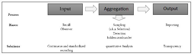
Data collection is prone to errors. Physician’s or patient’s reports may be (systematically) incorrect, creating a so-called observer bias, resp. recall bias. Both biases are measurement biases and cannot be corrected from an analytical perspective. Continuous tracking of the patient and standardized, quantifiable recording procedures in-time can reduce this bias, and IT platforms with automated data integrity and feasibility checks can improve data capturing quality, as employed in the case of the data base used in our example [22,23].

At the other end of the data analysis process, the output itself might be biased. Reporting bias is the most prominent output bias. It occurs when the reporting of research findings depends on their direction and nature. Studies with no significant effects rarely get published. To avoid this bias, all analyses must be pre-planned in a study protocol, which should be registered before any analyses are carried out (preferably for RWD-based studies in the ISPOR RWE registry; see ISPOR, 2021) [24].

The core element of the data analysis process is the aggregation of data (Table 1). The strongest biases usually appear in that category, leading to skewed data and reporting of spurious effects. Sampling bias (also known as selection bias) and detection biases are the most prominent biases in that category. An example of the detection bias is that physicians might be more likely to look for diabetes in obese patients than in skinny patients. As a result, one may observe an inflated estimate of diabetes prevalence among obese patients. To prevent the detection bias, core data elements need to be evaluated for a broad spectrum of individuals in a systematic manner. Selection bias occurs when the patients are assigned to different treatments in a non-random procedure. Here individual factors, like doctors´ experience or attitudes of doctors and patients, but also systemic factors like care algorithms or differences in availability results in the selection of a skewed treatment selection. Conclusions drawn from such a population sample cannot be generalized to the overall population.

Detection and selection biases can lead to (hidden) confounder bias. In RCT these biases are controlled for by inclusion and exclusion criteria as well as randomized assignment to interventional trials arms. In medical RWD-based studies many confounders, such as gender, age, physical condition, and others are known, depending on the field. The lack of randomization can be compensated by using a cohort matching technique such as pairwise propensity score matching of Rosenbaum and Rubin [25] employing these known confounders. For a non-mathematical introduction see [26-28]. Practical guidance is given by Loke and Mattishent [11]. Still the challenge of controlling the impact of hidden confounders remain, which is discussed in the following sections.

Confounding Bias

Example

A confounding bias occurs when an attribute (confounder) which is not included in the model influences (some of) the treatment as well as the output. In other words, the relationship between the treatment and the outcome is distorted by the confounder. Assume, for example, that patients who smoke tend to get a certain treatment, and smoking results in a higher disease activity, but smoking is not captured as relevant factor. This scenario leads to an underestimation of the treatment’s efficacy (Figure 1).

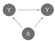
Figure 1: Example of confounding bias. Smoking (S) correlates with treatment choice (T) and response (Y).

To avoid such misjudgments, we need to account for all possible confounders. For example, a medical registry should contain standard attributes (e.g., age, gender, duration of disease, kind and duration of therapies, disease progression). Additionally, it cannot be ruled out that hidden confounders have an impact. It is difficult to evaluate the impact of these confounders, due to their invisible nature. Lin et al. [2] suggested a method to assess the sensitivity of regression results in the presence of hidden confounders. The following subsection shows how results with confidence intervals can be derived assuming a hidden confounder.

Theory Confounding Bias

Let Y∈{0,1} be a binary response variable (such as disease progression) and X∈{0,1} is the application of a certain treatment. Some covariates Z (e.g., age, gender) are measured while U∈{0,1} is a hidden binary confounder (assumed to be independent of Z). Let the probabilities of the hidden confounder differ in the treatment and the control group P(U=1|X=0)=p₀ and P(U=1|X=1)=p₁. If the probabilities are identical, the treatment group and the control group are equally affected by the confounder, such that the estimation of the treatment effect remains unbiased.

Consider the log linear model Pr⁡(Y=1│X,Z,U)=exp(α+βX+γU+θ’Z). As the hidden confounder is not estimated, the observed model Pr⁡(Y=1│X,Z)=exp(α*+β* X + θ*’Z) leads to estimates α*, β*, θ* which are potentially biased from the true parameters α, β, θ. Lin et al. found that the relationship between the observed treatment coefficient β* and the actual treatment coefficient β was given by

with Γ=e^γ being the relative risk of disease associate with the hidden confounder U. Similar results can be found for the logistic regression and for more general (such as normal distributed) confounders [2].

Real-world Application

Known Confounders

To determine the possible impact of hidden confounders, it is helpful to first evaluate the known confounders. This obviously depends on the context of the study. As the initial population of Braune et al. [1] was not available on patient level, we use a current data cut of the German NeuroTransData (NTD) Multiple Sclerosis registry, including patients with same inclusion characteristics as in the previously published population.

Our real-world application investigates relapse activity of patients with MS (PwMS). To estimate the impact of known confounders, we utilized a cross-sectional dataset sourced from the inception of the year 2022 (index date beginning of 2022) including 5679 active PwMS being on therapy on either Fingolimod, Interferon, Natalizumab or Ocrelizumab. Our binary depended variable states if there are relapses in the previous year or not (yes/no). We run a logistic regression of relapses on known established confounders (gender, age, Expanded Disability Status Scale (EDSS) at index date, number of treatments before index date and time since diagnosis to index date), as suggested by Karim et al. [20]. The result is given in Table 2.

Table 2: Results of logistic regression model of the event of a relapse on known confounders: Gender (female), Age (age), Expanded Disability Status Scale (EDSS), number of DMTs before index date (n.treatment) as well as time since diagnosis of MS in years (time.yrs). The point estimate is given as well as the standard deviation (Std.Error) and the corresponding p-value (Pr(>|z|)).

	Estimate	Std. Error	Pr(>|z|)
(Intercept)	-0.1451	0.1176	0.2176
female***	0.2156	0.0631	0.0006
age***	-0.0217	0.0028	<0.0001
EDSS_score***	0.1391	0.0206	<0.0001
n.treatments	-0.0294	0.0230	0.2012
time.yrs	0.0052	0.0105	0.6200

The most important confounder is gender. Based on our data, women have 24% (e⁰.2156=1.24) greater relative risk of relapses compared to men. 10 years increasing age leads to a 20% reduction of the relative risk. An EDSS score higher by one unit increases the relative risk by 15%.

Controlling these confounders as well as hidden confounders becomes crucial, if RWD are employed to comparatively analyze effectiveness of several drugs in a certain indication. While propensity score matching baseline variables can control for aggregation biases in RWD, still hidden confounders continue to challenge the robustness especially of comparative results.

Let there be a hidden confounder with a strong negative effect on the outcome. Assume first that it is equally distributed between all treatments. In this case, the confounder affects the treatment outcomes of different disease modifying therapies (DMTs) in relapsing remitting multiple sclerosis (RRMS) with the same magnitude in each treatment group, and the estimated efficacy of the treatments will be unbiased. Suppose now that the hidden confounder is more frequent in one treatment group than the other. Even if two treatments have a similar efficacy, one treatment will seem to be worse than the other.

It is crucial to determine how unequal known confounders are distributed, which is shown in Table 3 for each of the four DMT evaluated. For the therapies fingolimod (FTY), interferons (IFN), natalizumab (NAT) and ocrelizumab (OCR) the share of females, share of higher disability represented by higher EDSS (Expanded Disability Status Scale, mean EDSS score above the group mean 2.2), share of high age (age above the group mean of 39 years) is given. The share of females is relatively equally distributed over all therapies ranging from 62% to 76%, similar for the higher EDSS score (50% to 69%). The largest deviation in distribution is given for higher age, ranging from 37% to 59%.

Table 3: Distribution of well-known confounders (gender, above average EDSS score of 2.2 and above average age of 39 years) given different treatments fingolimod (FTY), interferon-ß (IFN), natalizumab (NAT), ocrelizumab (OCR). The strongest difference between treatment populations can be seen for above average age, ranging from 37% (NAT) to 59% (OCR).

Share (%)	FTY	IFN	NAT	OCR
Female	73%	73%	76%	62%
Higher EDSS	60%	50%	64%	69%
Higher age	53%	47%	37%	59%

In summary, well-known confounders in the field of MS treatments are found to increase the odds of responding to different DMTs by up to 25% and might be slightly unequal distributed (e.g. 40% to 60%) in different treatment groups. With this information, we can now check the results of previous findings in the literature in the presence of a potential hidden, hidden confounder.

Hidden (Potential) Confounders

For this exercise, we consider the results from the paper of Braune et al. [1]. The authors analyzed the comparative effectiveness of delayed-release dimethyl fumerate (DMF) against other treatments in patients with relapsing-remitting multiple sclerosis (RRMS) using propensity score matching. The results supported the superior effectiveness of DMF compared to interferons (IFN), glatiramer acetate (GA) and teriflunomide (TERI) and showed similar effectiveness to fingolimod (FTY). The pairwise comparisons of the paper are shown in the blue plot in Figure 2 (based on Figure 1 in Braune et al.). For IFN, GA and TERI, the rate ratio is significantly below 1, indicating better results for DMF.

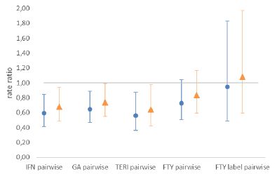
Figure 2: Hazard rate ratio of DMF vs. comparator. Rate ratios below 1 favor DMF.

Blue dots show hazard rate ratio as given in Braune et al. [1]. Orange triangles represent ratios given a large hidden confounder (p₀=0.4,p₁=0.6,Γ=2). The population of the therapies interferon-ß (IFN), glatiramer acetate (GA), teriflunomide (TERI), fingolimod (FTY) and the FTY (European) label are shown.

The propensity score matching accounts for the known established confounders such as sex, age, EDSS, disease duration, number of DMTs, and number of relapses in the past 12 and 24 months. While these are certainly the most influential confounders (Karim et al.) [20], an impact of additional hidden confounders cannot be excluded. Using the analysis described above, one can test if the results of Braune et al. [1] still hold in the presence of a hidden confounder. We know from our considerations above that common well-known confounders increase the odds by up to 25%. Consider an example of an extremely large confounder increasing the odds by 100% – or equivalently four perfectly correlated hidden confounders, each increasing the relative risk by 25%. In that case, we model the binary confounder with Γ=2. Note, that if the confounder appears at an equal rate in both groups (e.g. p₀=p₁), the measured comparative effectiveness is unbiased. Hence, assume that the hidden confounder is far more present in the comparator group (p₁=0.6) than in the DMF group (p₀=0.4 ). Given our analysis of known confounders in the previous section, a more unequal distribution of the hidden confounder in between the comparator and treatment group appears unlikely.

In such a scenario, the hidden confounder leads to an increase of effectiveness difference improperly in favor of DMF. We use the methodology presented by Lin et al. [2] to adjust for that effect. Figure 2 (orange triangles) presents the results in the presence of such an hidden confounder. For direct comparison also see Table 4.

Table 4: Hazard rate ratio for relapse activity during treatment with DMF vs. comparator including confidence intervals* (CI) excluding and including the adjustment of a binary confounder. The population of the therapies interferon-ß (IFN), glatiramer acetate (GA), teriflunomide (TERI), fingolimod (FTY) and the FTY (European) label are shown.

Comparison vs. DMF	Hazard Rate (CI) as published	Hazard Rate (CI) after confounder adjustment
IFN	0.59 (0.42,0.83)	0.68 (0.48,0.94)
GA	0.65 (0.48, 0.87)	0.74 (0.55,0.99)
TERI	0.56 (0.37,0.86)	0.64 (0.42,0.98)
FTY	0.73 (0.52, 1.02)	0.83 (0.60,1.17)
FTY label	0.94 (0.52,1.72)	1.08 (0.59,1.97)

* Note that the presented confidence bands differ slightly to the referenced paper due to different estimation procedures.

Because the impact of the hidden confounder leads to worse results for the comparator group (lower rate ratios), the rate ratios increase after the adjustment. To highlight IFN, the rate ratio increases from 0.59 to 0.68. Still, the qualitative conclusions of Braune et al. [1] that DMF has a higher efficiency than IFG, GA and TERI and similar efficiency to FTY remains, and the null hypothesis of equal effects of these two treatments is correctly rejected.

An arbitrarily strong hidden confounder can, of course, always change the results. See Table 5 for a comparison between DMF and IFN with hidden confounder Γ=2 and different distributions p₀, p₁ in the treatment and comparator group. For an equal distribution of the hidden confounder in the DMF and IFN population, i.e. p₀=p₁, the hazard ratio is given by 0.59 (as found by Braune et al.) [1] as both groups are equally exposed to the confounder. For a moderate divergence in both groups, e.g. em>p₀=0.4, p₁=0.6 the rate ratio is given (as mentioned before) by 0.68. For strong difference between both groups, with the DMF group being free of the hidden confounder (p₀=0) and the confounder group suffering strongly of the confounder (p₁>0.7) the effectiveness of DMF compared to the comparator reverses after the adjustment. IFN would then actually be more effective than DMF and only appear worse due to the hidden confounder. As Braune et al. [1] already control for all major known confounders, it seems unlikely that such a hidden confounder with such a massive impact exists. Note that the treatment differences of Braune et al. [1] further increase when the DMF group is more exposed to the confounder than IFN group, e.g. p₀>p₁.

Table 5: point estimates and confidence bands for hazard ratios for dimethylfumarat (DMF) vs. interferon-ß (IFN) adjusting for a hidden confounder with Γ=2 given the frequency of the confounder in the DMF group (p₀) and the comparator group (p₁). Result remains significant for italic cases.

	p1=0.0	p1=0.2	p1=0.4	p1=0.6	p1=0.7	p1=0.8	p1=1.0
p0=0.0	0.59 (0.43,0.83)	0.71 (0.51,0.99)	0.83 (0.6,1.16)	0.95 (0.68,1.32)	1.01 (0.72,1.4)	1.07 (0.77,1.49)	1.19 (0.85,1.65)
p0=0.2	0.49 (0.35,0.69)	0.59 (0.43,0.83)	0.69 (0.5,0.96)	0.79 (0.57,1.1)	0.84 (0.6,1.17)	0.89 (0.64,1.24)	0.99 (0.71,1.38)
p0=0.4	0.42 (0.3,0.59)	0.51 (0.36,0.71)	0.59 (0.43,0.83)	0.68 (0.49,0.94)	0.72 (0.52,1)	0.76 (0.55,1.06)	0.85 (0.61,1.18)
p0=0.6	0.37 (0.27,0.52)	0.44 (0.32,0.62)	0.52 (0.37,0.72)	0.59 (0.43,0.83)	0.63 (0.45,0.88)	0.67 (0.48,0.93)	0.74 (0.53,1.03)
p0=0.8	0.33 (0.24,0.46)	0.4 (0.28,0.55)	0.46 (0.33,0.64)	0.53 (0.38,0.73)	0.56 (0.4,0.78)	0.59 (0.43,0.83)	0.66 (0.47,0.92)

For some fixed confounder size Γ we can observe when the result loses significance. Figure 3 presents a graph for two different strengths of the confounder Γ∈(2.0,3.0). On the axis the frequency of the confounder in the comparator group (x-axis) and DMF group (y-axis) is given. The crosses indicate the maximum identified inequality in the distribution of the known confounders age, gender and EDSS between treatments (see also Table 3).

The practically most relevant question is under which circumstances the results of Braune et al. lose significance. For a certain confounder strength and inequality in the groups the significance of the found results by Braune et al. will not hold anymore. A confounder with Γ=1.2 (not shown in Figure 3) is too weak and cannot destroy the significance. That is noteworthy, because a 20% increase in relative risk is about the effect size found for the strongest known confounder (gender). An hidden confounder with Γ=2 impact the significance of the result, if the confounder is far more present in the comparator group (e.g. p₁>0.2) than the DMF group (e.g. p₀=0). For very large confounders the results could be reversed. A confounder with strength Γ=3.0 and a similar occurrence as the risk factor age would lead to the result being not significant anymore.

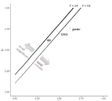
Figure 3: Illustration of threshold at which IFN loses significance to DMF for different strength of the hidden confounder with Γ∈(2.0,3.0) and different distribution of the confounder in the dimethylfumarat (DMF) group (p₀) and the comparator interferon-ß (IFN) group (p₁).

Summary and Conclusion

Findings in RWD can be distorted by several biases, including the confounding bias. We herein show how the methodology presented by Lin et al. can be applied in practice to analyze the significance of results in the presence of potential hidden confounders. First, we determined the effect size and distribution of known confounders. Our results underline the strong impact of the known confounders in multiple sclerosis, in line with previous reports (Karim et al.) and provide a quantitative base for the evaluation of the impact of hidden confounders. This analysis showed that a potential hidden confounder would have to exceed the impact of known confounders to such an extent, that its existence can be ruled out with almost certain probability. The method employed allows for different assumptions of equal and unequal distributions in the groups compared to understand the necessary strengths of hidden confounders to distort study results in different scenarios. Firstly, it is tested if the results hold in the presence of an hidden confounder as large as the known confounder. Then a threshold corridor can be defined, indicating quantitatively the limits of strengths of hidden confounder necessary for study results to lose their statistical significance. Considering previous work in this field, this method adds a new dimension by evaluating if the null hypothesis is still rejected after the confounder has been accounted for.

The presented method has some limitations. The first is the distribution assumption of the confounder. Lin et al. show that the method holds for binary and normally distributed confounders. For more extreme distributions with heavy tails, the applied correction might be insufficient. We further assume that hidden (or unmeasured) confounders have a similar distribution and strength as known confounders. However, if there is evidence that there are hidden confounders that are very unevenly distributed in the treatment populations or the hidden confounders might be of extreme strength, the method presented should not be applied.

The approach presented herein to battle the confounder bias can help increase the robustness and reliance of results from RWD. If observed effects are significant and the presented sensitivity analysis can show the robustness of the results in presence of a substantial confounding bias, decision makers can be more confident to rely on real-world evidence. RWD should thus not be dismissed a priori due to the “ghost of confounding,” because this ghost can be kept in check by quantitative methods shown herein applied to large-scale and robust datasets.

References

1. Braune S, Grimm S, van Hövell P, Freudensprung U, Pellegrini F, et al. (2018) Comparative effectiveness of delayed-release dimethyl fumarate versus interferon, glatiramer acetate, teriflunomide, or fingolimod: results from the German Neuro Trans Data registry. Journal of Neurology 265: 2980-2992. [crossref]
2. Lin DY, Psaty BM, Kronmal RA (1998) Assessing the sensitivity of regression results to unmeasured confounders in observational studies. Biometrics 948-963. [crossref]
3. Braune S, Rossnagel F, Dikow H, Bergmann A (2021) The impact of drug diversity on treatment effectiveness in relapsing-remitting multiple sclerosis (RRMS) in Germany between 2010 and 2018: Real-world data from the German NeuroTransData Multiple sclerosis registry. BMJ Open [crossref]
4. Bresalier RS, Sandler RS, Quan H, Bolognese JA, Oxenius B, et al. (2005) Cardiovascular Events Associated with rofecoxib in a Colorectal Adenoma Chemoprevention Trial. The New England Journal of Medicine 352: 1092-1102. [crossref]
5. O’Leary CP, Cavender MA (2020) Emerging opportunities to harness real world data: An introduction to data sources, concepts, and applications. Diabetes Obes Metab 22: 3-12. [crossref]
6. FDA (2021) Real-World Evidence. Office of the Commissioner. https://www.fda.gov/science-research/science-and-research-special-topics/real-world-evidence. Accessed April 27, 2023.
7. Bakker E, Plueschke K, Jonker CJ, Kurz X, Starokozhko V, Mol PG (2023) Contribution of Real-World Evidence in European Medicines Agency’s Regulatory Decision Making. Clin Pharmacol Ther 113: 135-151. [crossref]
8. Mahendraratnam N, Mercon K, Gill M, Benzing L, McClellan MB (2021) Understanding Use of Real-World Data and Real-World Evidence to Support Regulatory Decisions on Medical Product Effectiveness. Clinical Pharmacology & Therapeutics 111: 150-154. [crossref]
9. Gray CM, Grimson F, Layton D, Pocock S, Kim J (2020) A Framework for Methodological Choice and Evidence Assessment for Studies Using External Comparators from Real-World Data. Drug safety 43. [crossref]
10. Baumfeld AE, Reynolds R, Caubel P, Azoulay L, Dreyer NA (2020) Trial designs using real-world data: The changing landscape of the regulatory approval process. Pharmacoepidemiology and Drug Safety. [crossref]
11. Loke YK, Mattishent M (2020) Propensity score methods in real-world epidemiology: A practical guide for first-time users. Diabetes Obes Metab 22: 13-20. [crossref]
12. Varga AN, Guevara Morel AE, Lokkerbol J, van Dongen JM, van Tulder MW, et al. (2023) Dealing with confounding in observational studies: A scoping review of methods evaluated in simulation studies with single‐point exposure. Statistics in medicine 42. [crossref]
13. Zhang X, Faries DE, Li H, Stamey JD, Imbens GW (2018) Addressing unmeasured confounding in comparative observational research. Pharmacoepidemiol Drug Saf 27: 373-382. [crossref]
14. Zhang X, Stamey JD, Mathur MB (2020) Assessing the impact of unmeasured confounders for credible and reliable real-world evidence. Annu Rev Public Health 5.
15. Groenwold RHH, Sterne JA, Lawlor DA, Moons KG, Hoes AW, et al. (2016) Sensitivity analysis for the effects of multiple unmeasured confounders. Ann Epidemiol 26. [crossref]
16. Popat S, Liu SV, Scheuer N, Hsu GG, Lockhart A, et al. (2022) Addressing challenges with real-world synthetic control arms to demonstrate the comparative effectiveness of Pralsetinib in non-small cell lung cancer. Nat Commun 13: 3500. [crossref]
17. He W, Fang Y, Wang H (2023) Real-World Evidence in Medical Product Development. Springer Nature.
18. Mathur MB, VanderWeele TJ (2022) Methods to Address Confounding and Other Biases in Meta-Analyses: Review and Recommendations. Annual Review of Public Health 43: 19-35. [crossref]
19. Leahy TP, Kent S, Sammon C, Groenwold RH, Grieve R, et al. (2022) Unmeasured confounding in nonrandomized studies: quantitative bias analysis in health technology assessment. J Comp Eff Res 11: [crossref]
20. Karim ME, Pellegrini F, Platt RW, Simoneau G, Rouette J, et al. (2022) The use and quality of reporting of propensity score methods in multiple sclerosis literature: A review. Mult Scler 28: 1317-1323. [crossref]
21. Kalincik T, Butzkueven H (2016) Observational data: Understanding the real MS world. Mult Scler 22: 1642-1648. [crossref]
22. Bergmann A, Stangel M, Weih M, van Hövell P, Braune S, et al. (2021) Development of Registry Data to Create Interactive Doctor-Patient Platforms for Personalized Patient Care, Taking the Example of the DESTINY System. Digit. Health 3: 633427. [crossref]
23. Wehrle K, Tozzi V, Braune S, Roßnagel F, Dikow H, et al. (2022) Implementation of a data control framework to ensure confidentiality, integrity, and availability of high-quality real-world data (RWD) in the NeuroTransData (NTD) registry. JAMIA Open 5: ooac017. [crossref]
24. ISPOR (2021) Real-World Evidence Registry. https://www.ispor.org/strategic-initiatives/real-world-evidence/real-world-evidence-registry. Accessed April 27, 2023.
25. Rosenbaum PR, Rubin DB (1983) The Central Role of the Propensity Score in Observational Studies for Causal Effects. Biometrika 70.
26. Franchetti Y (2022) Use of Propensity Scoring and Its Application to Real-World Data: Advantages, Disadvantages, and Methodological Objectives Explained to Researchers Without Using Mathematical Equations. J Clin Pharmacol 62. [crossref]
27. Cohen JA, Trojano M, Mowry EM, Uitdehaag BM, Reingold SC, et al. (2020) Leveraging real-world data to investigate multiple sclerosis disease behavior, prognosis, and treatment. Mult Scler 26.
28. Lin KJ, Rosenthal GE, Murphy SN, Mandl KD, Jin Y, et al. (2020) External validation of an algorithm to identify patients with high data-completeness in electronic health records for comparative effectiveness research. Clinical Epidemiology 12: 133. [crossref]