DOI: 10.31038/AFS.2019111
Abstract
The cultivation of macroalgae in earth ponds could provide an optimal control on both quantity and quality of biomass. In previous studies the genus Ulva has proved to be an ideal candidate for growing in fish ponds since it withstands their considerable environmental fluctuations. This study assessed the biomass production and the SGR (specific growth rate) of green algae Ulva sp. cultivated in earth ponds facing the Ria Formosa lagoon (Southern Portugal). The growth and production performance were tested among: a) two different multitrophic systems (IMTA (fish +oyster + Ulva) and ‘Fish + Ulva’); b) four different initial densities (15 ,30, 50 e 60 g/m2); c) five production and harvest cycles (6, 7, 8, 9 e 15 days). The Specific Growth Rate (SGR) of Ulva sp. was found to be significantly different between the two multitrophic systems (p <0.05) and higher in the ‘Fish + Ulva’ system (19.3 ± 0.08% day-1) than in the IMTA system (16.7 ± 0.8% day-1). Also, there were significant differences between different densities and varied cultivating periods. Growth of Ulva sp. was dependent on both densities and time periods. The densities of 30g/m2 revealed to be the best among the four tested densities (23 ± 3.9 % day−1) whereas the optimal cultivating period was between seven and nine days (≈21 % day−1). The experiments on the production cycle indicated an optimal period of cultivation of about 8 days.
Keywords
Ulva sp.; Biomass production; Specific Growth Rate (SGR); Integrated Multitropihc Aquaculture (IMTA).
Introduction
Despite the growing demand for algae in the EU markets, its production is growing slowly with respect to the world’s largest producers [1]. Traditionally, both in Europe and in Portugal, the macroalgae industry was based mainly on the harvesting of macroalgae [1,2]. However, this technique is subject to annual fluctuations, poor product quality and raises concerns about the conservation of the marine ecosystem [1]. The cultivation of macroalgae in earth ponds and tanks could provide a better control on both quantity and quality of biomass [3–5]. The genus Ulva has proved in previous studies to be an ideal candidate to growing in fish ponds since it reaches high biomass production with high protein content [4, 6–8]. The rapid growth of Ulva is attributed to its high photosynthetic rates and high ability to uptake dissolved nitrogen [8]. Ulva withstands the considerable environmental fluctuations to which the tanks or ponds are subjected [4,9]. Additionally, the environment of the ponds is improved by this type of macroalgae which is able to balance fishpond pH level, oxygen demand and to increment chlorophyll a concentration [4,10]. There is always certain seasonality in growth capacity and biomass yield of Ulva [11]. Seasonality is especially important in the tank cultivation of Ulva in temperate zones as all factors, environmental and ecological, vary considerably [12]. Ulva has long been integrated into land based Integrated Multi-Trophic Aquacultures (IMTA) for biomass production and bioremediation [13]. Since Growing Ulva in effluent media increases its protein content (> 40%), it turned out to be a valuable feed for macroalgivores* species with high commercial value [8,13,14]. Currently the market for these algae is limited, but studies that discuss the suitability of Ulva as a biomass energy resource and its application as a raw material for nutraceuticals, biomaterials and sulphated polysaccharides (ulvan), can increase their attractiveness [13–15]. The present work focused on the feasibility of integrating a land-based production system of Ulva sp. on a semi-commercial aquaculture farm, with the objective of assessing the Specific Growth Rate (SGR) and Biomass production of Ulva sp. in multitrophic aquaculture.
Materials and Methods
Ulva sp. Production
The multitrophic aquaculture experiment was conducted at the Aquaculture Research Station in Olhão (EPPO- Estação Piloto de Piscicultura de Olhão), Portugal. Four rectangular 450 m2 x 1.5 m deep earthen ponds were used: 2 with fish, oyster and macroalgae (IMTA) and 2 without oysters (Fish + Ulva) (Figure 1). Autotrophs (phytoplankton, Ulva sp.), filter-feeding species (Crassostrea gigas) and fed organisms (Argyrosomus regius, Mugil cephalus, Diplodus sargus) are grown in the same earthen pond. Stock densities of the organisms cultivated are showed in table 1.

Figure 1. Pattern of assay in EPPO earth ponds.
Table 1. Stock densities of the organisms present in the pond.
|
Species |
Density |
|
Argyrosomus regius |
1500 (N°/pond) |
|
Diplodus sargus |
900 (N°/pond) |
|
Mugil cephalus |
550(N°/pond) |
|
Crassostrea gigas |
18000 (N°/pond) |
|
Ulva sp. |
30g/m² x 6 rafts |
Growth, biomass production and best cultivation period were evaluated for the cultivated macroalgae belong to the genus Ulva (Linnaeus, 1753). The time scheduled for the several experiments is shown in Figure 2) The first experiment involved the evaluation of the best stock density for Ulva’s growth; 2) The best cultivation time to attain the highest growth (best cultivation Period) was determined next in a specific experiment where daily production of Ulva sp. was followed for 8 consecutive days (dry biomass was also measured); 3) After determining this density, the production of Ulva in the ponds was assessed by comparing the multitrophic system IMTA and Fish+Ulva.
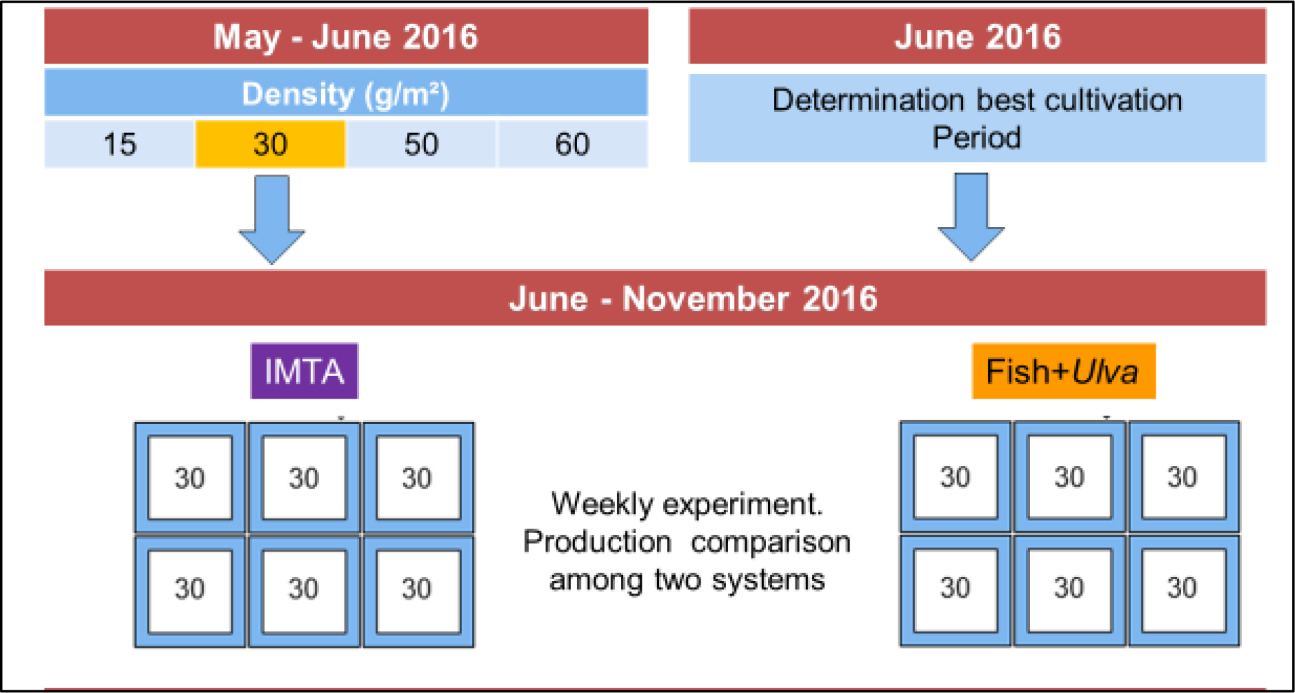
Figure 2. Time schedule of experiments ran during the study
Naturally occurring Ulva was collected in the main discharge channel and in the settling pond of EPPO (Figure 3a). After harvest, the macroalgae were washed with clean saltwater to remove most of the impurities and epibionts and drained by excess water. A portion of the harvest was weighted and individually planted in 6 rafts, each measuring 1 m2, made of horizontal nets stretched between styrofoam floaters. The individual pieces of macroalgae were attached to the net with brackets (Figure 3b and 3c).
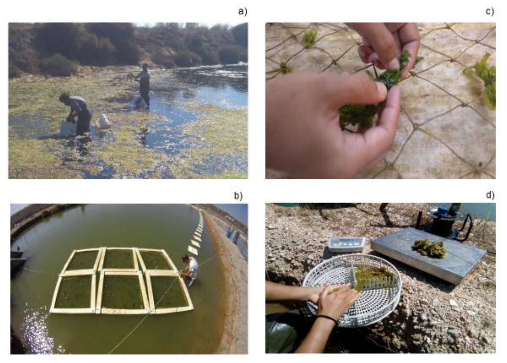
Figure 3. a) Collecting Ulva sp. from discharge channel; b) the six floating rafts; c) Ulva being fixed with brackets; d) macroalgae draining and weighing.
The stock density that permitted the highest growth of Ulva was determined in May-June 2016 in a three-weeks trial to evaluate the growth of the macroalgae (Figures 2 and 4). Specific Growth Rate (SGR) and Wet Biomass Production (WBP), was tested using four stock densities: 60, 50, 30 and 15 g/m2. Each week the growth obtained with different stock densities (60, 50 e 15 g/m2) were compared with the growth obtained with 30g/m2 that act as a control for comparison. This was done to prevent the effect of differences in environmental conditions among the three experiments. Ulva was distributed among the six rafts in the way shown in Figure 4. Since the 30g/m2 showed the best results it was decided to plant the floating structures with this density in all subsequent experiments.

Figure 4. Scheme representing the density distribution in the six rafts.
To determine the cultivation time for highest growth the SGR was obtained for 5 different cultivation periods: 6, 7, 8, 9 and 15 days in June 2016. This allowed drawing a growth curve to define the cultivation time that resulted on better growth rates. To accurately determine the daily growth curve another experiment was carry out on an eight-day experiment where the macroalgae biomass was sampled daily. The experiment started on June 2016. Eight floating rafts (each of 1m2) were placed in a pond containing oysters and fishes (Figure 5). In the following eight days, a raft was chosen at random and the macroalgae removed, washed, drained and weighed. In this experiment the water temperature (°C), pH, turbidity (FNU) and dissolved oxygen (ppm and % saturation) were determined twice a day. Ulva sp. were collected, washed and weighed as in previous experiments. 30g of macroalgae was placed on each raft and 3 samples of 30g, were dried up in an oven at 60°C to obtain an average starting dry weight. Obtaining the dry weight allowed to calculate the percentage (17.7%) of dry biomass presents in the wet Ulva biomass collected as follow: (DW/WW) *100. The dry weight (DW) was determined by drying the algae at 60°C in a hoven. Dry biomass production (DBP) was calculated by the following equation:
DBP = [(DWf–DWi)/(A*t)]
where DWf = final dry weight, DWi = initial dry weight, t = days of culture and A = culture area [16].
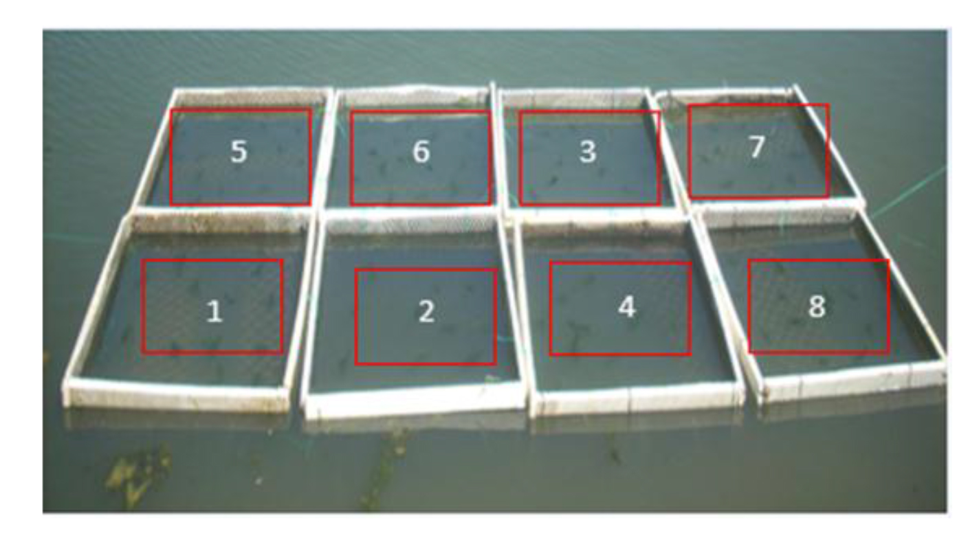
Figure 5. Eight-days experiment to determine the growth period. Each raft had 30 g/m2 of initial density. Every number represents after how many days the algae were harvested from that raft.
From June to November 2016 the production of IMTA and Fish+Ulva systems was compared. A total of 14 weekly harvests were carried out. During the experiment water temperature (°C), pH, turbidity (FNU, Formazin Nephelometric Units) and dissolved oxygen (ppm and % saturation) were measured with multiparameter probes (Hanna Instruments H9829) twice a day. The irradiance was measured using an Apogee Mark Model SP-214 pyranometer. Furthermore, monthly, samples were taken to determine the concentration of Chlorophyll a and nutrients (NH4, NO3–, NO2–, HPO4–). The nutrients were analysed by colorimetry method (Grasshoff et al., 1983) whereas Chlorophyll a was determined by spectrophotometry according to Parsons et al. (1984).
Macroalgae harvesting was done by hand. The floating structures were gently agitated to remove deposited sediments on the surface of the macroalgae before harvest. Prior to weighing Ulva was washed with filtered salt water to remove debris and epibionts, squeeze drained and the biomass in each 1 m2 determined individually in a scale with a 1 mg accuracy (Figure 3d).
The daily wet biomass production (WBP) at each 1 m2 raft composing the floating structure was calculated and expressed in g m−2 day−1.
Specific growth rate (SGR, %) of Ulva in the rafts was calculated as:
SGR = ln (WWt–WWi)/t
where WWi is the initial wet weight and WWt is the wet weight after t = time (cultivation days).
Statistic
The normality (Shapiro-Wilk’s test) and homogeneity of variances (Bartlett’s test) within the biotic and abiotic factors were tested before applying parametric test. When these assumptions were not respected, the non – parametric test (Kruskal – Wallis) was used. Statistical test of one-way ANOVA within abiotic factors was performed to identify the possible differences between the two production systems [17]. One-way ANOVA was also used to test the Specific Growth Rate (SGR) obtained from the two different systems.
The SGR (specific growth rate) of the two systems was used for the following statistical test:
- To determine the correlation (with Spearman variant in case of no normality-homogeneity) between physic-chemical parameters in the pond water and SGR.
- To assess the different densities and periods of cultivation. In this case when statistical difference was found a pairwise test was done to know which groups cause the difference (‘inhomogeneity’) [17].
Values for dissolved oxygen, pH, temperature and turbidity used in the correlation analysis (see Figure 7 in Results) correspond to the daily mean of a seven days period prior to the sampling for the other parameters.
Results
Ulva sp. Production
Abiotic factors (Table 2)
Table 2. Mean ± standard deviation values of abiotic and biotic factors for the two systems (IMTA and Fish + Ulva), and level of significance (p-value) of the comparison between the two using one-way ANOVA.
|
System |
IMTA |
Fish + Ulva |
p-value |
|
Factor |
|||
|
Temp.(°C) |
25.11±2.92 |
25.08±2.85 |
p>0.05 |
|
pH |
8.47±0.19 |
8.43±0.17 |
p<0.01 |
|
D.O. (ppm) |
5.92±1.03 |
5.67±0.98 |
p<0.01 |
|
Turb. (FNU) |
17.91±7.20 |
20.59±8.44 |
p<0.001 |
|
Irr.a (kW m-2) |
400.47±288.5 |
400.47±288.5 |
– |
|
Sal. (psu) |
36.08±0.85 |
36.04±1.76 |
p>0.05 |
|
NH4+(µM) |
32.20±22.67 |
36.89±8.63 |
p>0.05 |
|
NO3– (µM) |
7.84±5.18 |
6.02±1.73 |
p>0.05 |
|
HPO4–2 (µM) |
1.02±0.02 |
0.93±0.33 |
p>0.05 |
|
NO2–(µM) |
1.42±1.12 |
1.37±0.61 |
p>0.05 |
|
Chla (µg/l) |
1.07±0.63 |
0.86±0.66 |
p>0.05 |
a.Irradiance equal for both systems because the data came from meteorological station placed on the roof of EPPO building.
The temperature of the water averaged 25.11±2.92 ºC and 25.08±2.85 ºC at IMTA ponds (Fish + Oysters + Ulva) and at ponds without oysters (Fish + Ulva) respectively. During the experience, the temperature range between 30.2°C (maximum value found on IMTA ponds on July) and 15.5°C (minimum value found on Fish + Ulva ponds on November). Salinity was almost constant (≈ 36 PSU) except on the last day of October when it was raining (minimum value of 32.26 PSU). No significant difference was found between the ponds and systems respecting the temperature and salinity (p>0.05).
pH and dissolved oxygen (D.O.) in the water increased on the ponds from morning to afternoon, and this difference was more pronounced during summer (Figures 6a and 6b). Dissolved oxygen and pH presented higher mean values in the IMTA ponds (pH = 8.47±0.19; D.O.= 5.92±1.03) when compared to Fish + Ulva ponds (8.43±0.17; D.O.= 5.67±0.98) and in October when there was a peak at IMTA ponds for both parameters. Either D.O. and pH presented significant difference between the systems (p<0.01). Also for the turbidity (FNU) was statistically different among systems but in this case the higher mean corresponded to Fish + Ulva system (20.59±8.44). Mean values of nutrients and chlorophyll a are presented in Table 2. No significant differences were found between the systems for these factors. Both temperature and pH showed a positive correlation with specific growth rates (SGR), whereas a negative correlation was found between SGR and NH4+( p-values< 0.05) (Figure 7). Values for dissolved oxygen, pH, temperature and turbidity used in the correlation analysis correspond to the daily mean of a seven days period prior to the sampling for the other parameters.
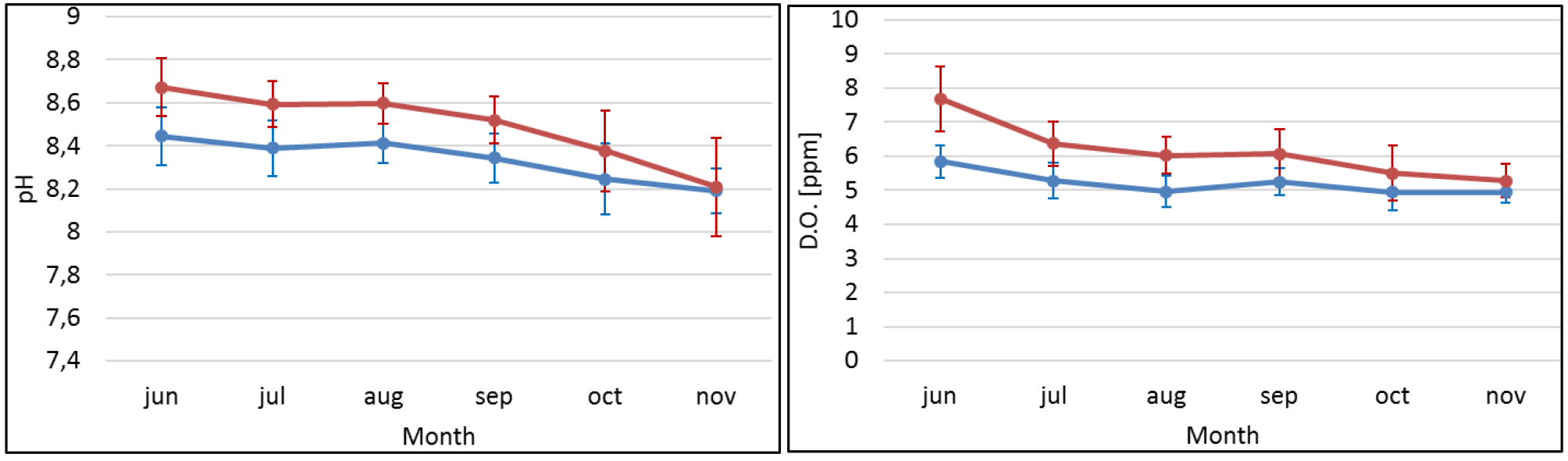
Figure 6. Means of daily variation of pH(a) and D.O(b) in the ponds (morning, blue lines; afternoon, red lines) during the 5 months of the experiment (systems are represented together). Vertical bars represent standard deviation.
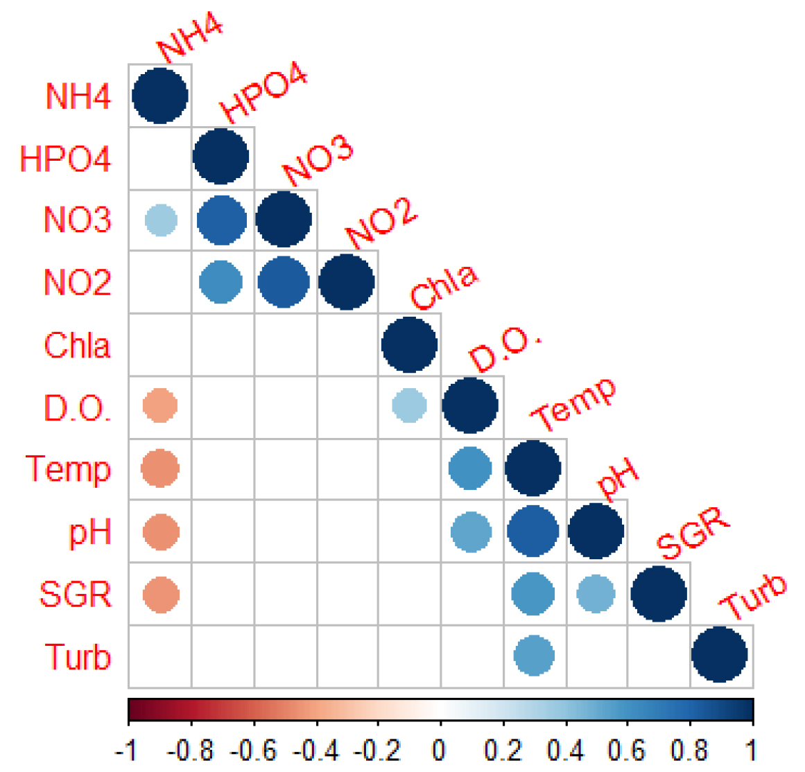
Figure 7. Correlation between biotic and abiotic parameters in the ponds. Correlations with p-value > 0.05 were considered as non-significant and leaved blank. Circles represent significant correlations: red – negative correlation, blue – positive correlation. Colour intensity and size of the circles are proportional to the significance of the correlation coefficient. (NH4+, HPO4–2, NO3–, NO2– in µM: Chlorophyll a in µg/l; D.O.: dissolved oxygen in µM; Temp: temperature in °C; SGR: specific growth rate in %, Turb: turbidity in FNU).
Ulva sp. growth and biomass yield
Specific growth rate (SGR) of Ulva sp. had a mean of 19.3±0.08% at Fish + Ulva ponds and 16.7±0.8% at IMTA ponds. Kruskal-Wallis test gave a narrow significant difference between the systems (KW=3.85, p=0.049). The maximum SGR of Fish + Ulva systems was achieved on 13 September (36.51%), whereas IMTA registered the higher value on 19 July (31.33%) (Table 3).
Table 3. Specific growth rate (SGR) and daily wet biomass production (WBP) during the experiment. Kruskal-Wallis (KW) value and significance (p).
|
System |
Min value |
Mean ± SD |
Max value |
KW |
p-value |
|
SGR (% d-1) |
|||||
|
IMTA |
5.6 |
16.7±0.8 |
3.33 |
3.85 |
p<0.05 |
|
Fish+Ulva |
3.0 |
19.3±0.08 |
36.51 |
||
|
WBP |
Min value |
Mean ± SD |
Max value |
KW |
p-value |
|
IMTA |
0.25 |
12.3±9.89 |
44.85 |
5.84 |
p<0.05 |
|
Fish+Ulva |
0.74 |
17.2±13.60 |
65.87 |
The mean wet biomass production (WBP) created by the two systems were statistically different (KW=5.84, p<0.05) with a maximum value found on Fish + Ulva ponds of 65.87 g m-2d-1 on 13 of September (Table 3).
Figures 8 and 9 show two clear cycles of increase and decrease for both SGR and WBP that corresponds to 6 weeks each. The first increase started in June 24 peaking in 19 July followed by a decrease until August 11 when it reached the minimum value; after this date they started increasing again until September 02. The second decrease reached the minimum value in October 20. The SGR followed the temperature fluctuation only in the last period of the experiment, whereas the ammonium variation is clearly in opposition to the biomass production (Figure 9).
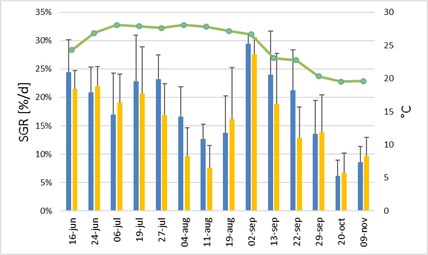
Figure 8. Variation of specific growth rate (SGR) (at right) of Ulva sp. along the experiment. X axis refers to day of harvesting. The green line represents the average water temperature during the 7 days of the cultivation periods (at left). Blue bars: Fish + Ulva system; Yellow bars: IMTA system; lines: standard deviation.
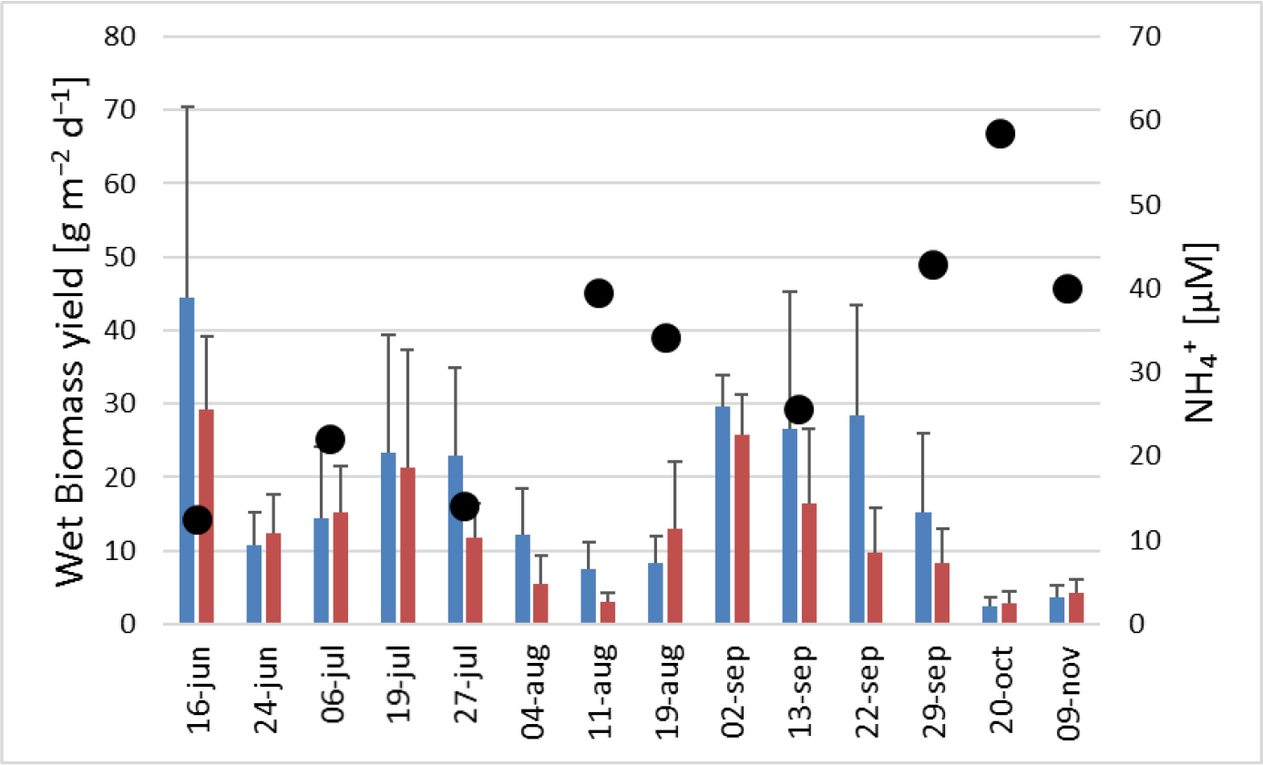
Figure 9. Variation of Wet biomass production (WBP) (at right) of Ulva sp. along the experiment. The black dots correspond to the ammonium concentration (at left) in the tanks during the sampling day. Blue bars: Fish + Ulva system; red bars: IMTA system; lines: standard deviation
Best Cultivating Periods and Stock Densities for Improved Growth
The Figure 10 shows a polynomial trend line of 2nd order (an ascending curve) to illustrate the relationship between the five different cultivation periods and their SGR. The coefficient of determination R2= 0.9474 represents the fitting of the data to the line. The SGR between the 5 cultivating periods were found to be statistically different (KW = 25.045, p<0.001) and the pairwise test stressed that the 6 and 9 days were those that differed significantly from the other three (p=0.0018) (Table 4). The SGR of Ulva sp. of the 7–8-9 days periods were almost double of the remaining two (Figure 10). Abiotic parameters during the experiment to determine the best cultivating period are shown in Table 5.
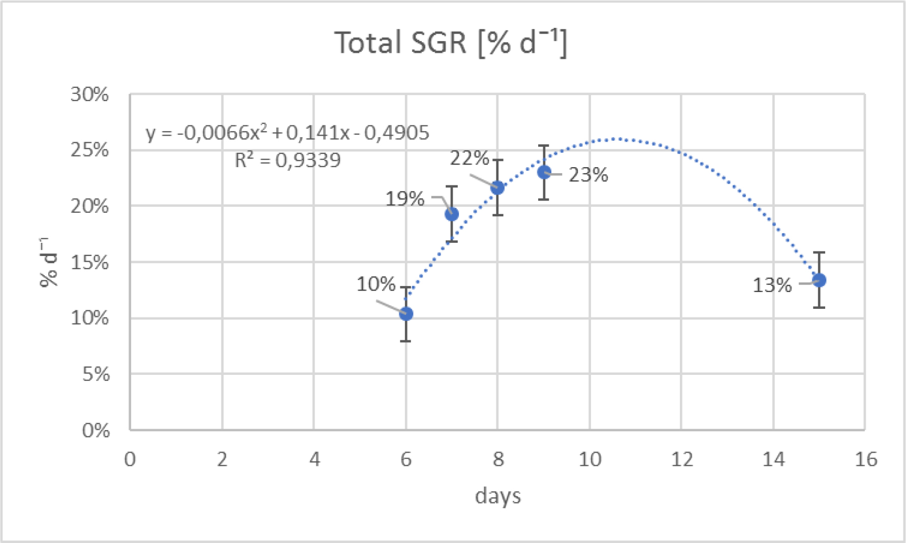
Figure 10. Growth curve using SGR recorded from 5 different cultivation periods.
Table 4. Numeric matrix containing the p-values of the t- tests calculated for each pair of cultivation period groups. In the output view, the red numbers stressed the periods are significantly different from each other (p<0.05).
|
Cultivation period |
6 days |
7 days |
8 days |
9 days |
15 days |
|
6 days |
— |
||||
|
7 days |
0.018 |
— |
|||
|
8 days |
0.2109 |
1.0000 |
— |
||
|
9 days |
0.0018 |
1.0000 |
1.0000 |
— |
|
|
15 days |
1.0000 |
0.1127 |
0.7544 |
0.0058 |
— |
Table 5. Mean values (8 days) of abiotic parameters during the experiment to determine the daily growth.
|
System |
Temp.(°C) |
pH |
D.O. |
Turb. |
Sal. |
|
Morning |
25.2±0.81 |
8.2±0.05 |
4.6±0.77 |
15.9±1.71 |
36.5±0.07 |
|
Afternoon |
26.9±1.93 |
8.5±0.06 |
8.4±2.03 |
19.2±1.88 |
36.6±0.07 |
Different stock densities did show differences for SGR and for WBP (KW= 24.343, p<0.05) (Table 6). The values for 60 grams were omitted due to a measurement error during weighing. For the densities, the pairwise test showed a significant difference in biomass production between 30g/m2 and the lower value (15 g/m2) (p = 0.0004) but not with 50 g/m2 (Table 7).
Table 6. Specific growth rate (SGR) and wet biomass production (WBP) obtained with 3 different initial densities
|
15 |
30 |
50 |
|
|
SGR(%/d) |
21.1 ± 4.8 |
23.0 ± 3.9 |
15.7 ± 7.6 |
|
WBP(g/m2d) * |
6.9 ± 2.9 |
22.2 ± 12.6 |
17.40 ± 13.4 |
*Significant difference p<0.05
Table 7. Numeric matrix containing the p-values of the t- tests calculated for each pair of stock densities groups. In the output view, the red numbers stressed the biomass are significantly different from each other (p<0.01).
|
Densities |
15g/m2 |
30g/m2 |
50g/m2 |
|
15g/m2 |
— |
||
|
30g/m2 |
0.0004 |
— |
|
|
50g/m2 |
0.004 |
0.312 |
— |
Daily Growth of Ulva sp.
Daily growth rates (SGR), obtained during the 8 days experiment, are presented in Figure 11. The SGR increased linearly until the third day of cultivation (R2=0.9969) then entered a stationary phase (R2=0.0883) with values identical or slightly lower than those reached on the third day (≈ 39 %). The daily increase of dry weight (DW) followed an exponential curve (R2=0.9756) (Figure 12) until the seventh day then slow down sharply. The dry and wet biomass productions on the 8th day was 10.9 g m-2d-1 and 60.6 g m-2d-1 respectively.
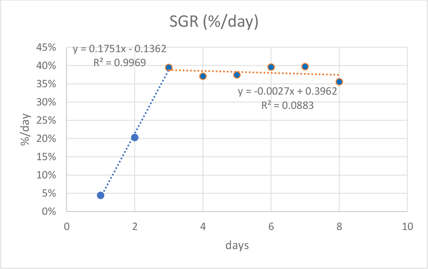
Figure 11. Growth curve of Ulva sp. SGR grown in eight-days experiment. Blue line represents first 3 days trend. Orange line represents the last 5 days.
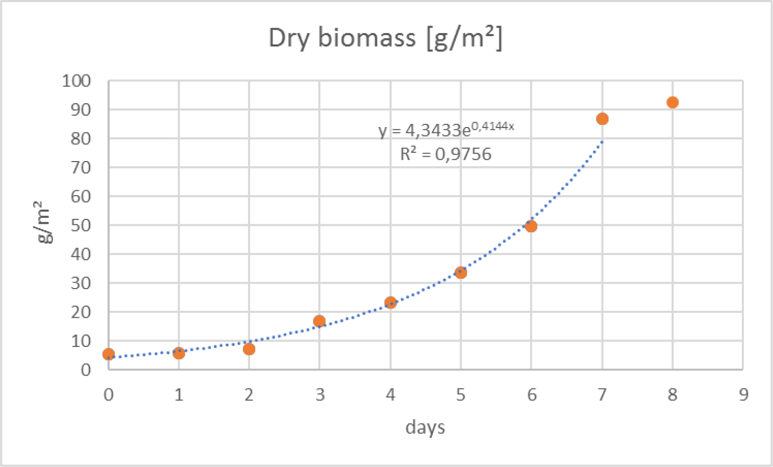
Figure 12. Growth curve of Ulva sp. dry biomass (DW) grown in eight-days experiment.
Discussion
EPPO pond water and their abiotic factors supported well the Ulva sp. growth. The values of specific growth rate (SGR) of both systems gave results similar to other studies (Table 8). However, the wet biomass production (WBP) and the Dry Biomass Production (DBP) recorded in this experiment were often lower than the others likely due to the use of different tank sizes, techniques or different initial density of Ulva [16,19] .
Table 8. Comparison of averages of specific growth rate(SGR), dry biomass production (DBP), Wet biomass production(WBP) cultured in different systems with different stock density (Table adapted from Ben-Ari et al., 2014 [8] and Castelar et al., 2014 [16]).
|
Species |
System |
Stocking density (kg WW m-2) |
DBP |
SGR |
WBP |
References |
|
Ulva sp. |
Earth pond |
0.06–0.015 |
2.6 |
17 |
14.75 |
This study |
|
Ulva lactuca |
Tank |
1–8 |
34.5–6 |
10–1 |
230–40 |
Bruhn et al., 2011 [14] |
|
Ulva sp. |
Ropes,sea |
0,0005* |
0.24 |
11.95 |
_ |
Castelar et al., 2014 [16] |
|
Ulva sp. |
Tank |
0,0005* |
0.47 |
22.80 |
_ |
Castelar et al., 2014 [16] |
|
Ulva clathrata |
Tank |
0.2–0.5 |
10.5 |
7 |
70 |
Copertino et al., 2009 [22] |
|
Ulva lactuca |
Tank |
1 |
16.8 -56.4 |
_ |
112–376 |
Msuya and Neori, 2008 [18] |
|
Ulva lactuca |
Tank (continuous aeration) |
0.8 |
47.7 |
13.3 |
318 |
Ben-Ari et al., 2014 [8] |
|
Ulva lactuca |
Tank (25% aeration) |
0.8 |
26.7 |
8.1 |
178 |
Ben-Ari et al., 2014 [8] |
The optimal cultivation period into EPPO ponds seemed to be positioned between seven to nine days since, after this time, the SGR decreased. Moreover, looking at the growth curve of Dry Weight (DW) obtained after eight days cultivations, Ulva sp. seemed to have reached the maximum of biomass around this period. This result and SGR values greater than 10% up to 15 days of cultivation suggest a production cycle of approximately 8 days.
The SGR and WBP during the experience drew a sinusoidal pattern with two spikes and two falls of values. The drop in autumn can be explained by a decrease in temperatures and a reduction of light period [20,21], in addition to a week of rain that occurred before the last collection. More complicated is explaining the drop in August. During this period was noted the presence of white spots in the Ulva thalli a phenomenon known as “ghost tissue” often indicative of an increase in sporulation. Sporulation can be caused by several factors such as elevated temperatures, irradiance, lack of nutrients and life cycle’ stage [22,23]. However, temperature and irradiance were constant from June to the end of August and the first one was within the optimum range for the species [16,24]. Even pH values (7.6<pH<8.8) were optimal for species growth, since they could be related to a high presence of dissolved bicarbonate (HCO3–) in water, the main source of inorganic carbon for the seaweed [25–27]. Therefore, life cycle could explain the August decreased. A study concerning Ulva rigida conducted in the Venice lagoon reported pulses of production during the year similar to that of this study [28]. The algae could have been harvested at a specific stage of the life cycle and the procedure to weigh it and put it in the structure could have accelerated these sporulation processes [23,29]. Although the nutrients concentration of EPPO ponds was like if not greater than previous studies [11,16,20,30,31] cannot be ruled out the possibility of a shortage of nutrients, particularly of NH4+. The increasing concentration of NH4+ during the phases of decline in algal biomass (Figure 3.3b) could represent a phase of renewal of nutrients up to a re-optimal level for algae. Another hypothesis would suggest that this oscillation depicted the Ulva sp. capacity to remove this nutrient. When macroalgae biomass declined the assimilative capacity of the environment for nutrients declined in turn. However, specific studies will be required for a proper evaluation of both conclusions.
Initial different densities showed better results for 30g/m2 which led to the decision discussed in the methodology (see Material and methods). Using low initial density has been suggested as a possible optimization of growing space [16]. Nevertheless, in macroalgae culture it’s usually used an optimum initial density of 1 kg/m2 but growing macroalgae in tanks equipped with artificial aeration to ensure there is no shading among the algae [8,14].
Ulva growing in the ‘Fish + Ulva’ system revelled a better performance than in the IMTA. ‘Fish + Ulva’ system presented mean values superior for both SGR and WBP. Since environmental parameters such as temperature, salinity and irradiance were identical for both systems the cause could be attributed to interactions between the different organisms presents into the ponds. It is known that oysters remove suspended particle by filtration [32] which explains the turbidity difference between the two systems. However, they contribute to the N pool with their excretions [33] so there might be higher growth of phytoplankton with limitations in the growth of Ulva in IMTA system. Nevertheless, the presence of oysters may have also caused a variation in the bacterial community [33,34]. Since the rule of bacteria is important for the growth and the morphogenesis of some species of green algae [15,35,36] the variation in quantity and quality of their community could have affected the growth of algae.
Wet biomass values were converted to dry biomass considering that dry/wet Ulva sp. biomass is around 15 % (17.7 %in this study); *dry biomass.
The differences in oxygen concentrations and pH between early morning and afternoon stressed the ability of the primary producers, Ulva sp. included, to oxygenate the water in both systems.
Conclusion
Ulva sp. showed to grow well under conditions typical of earth-pond aquaculture. The experiments on the production cycle indicated a period of cultivation of macroalgae of about 8 days. Despite the differences found within the systems, the growing periods and the initial densities of Ulva sp., the growth values have always been satisfactory. The technique used for cultivation has proved feasible. However, it will be necessary to assess the growth of the species along the year to evaluate better it response at environmental changes. Even higher stock densities should be tested to evaluate a possible cultivation for commercial purposes.
References
- EUMOFA (2016) Monthly Highlights – October, (April) 23 (www.eufoma.eu).
- Pereira L, Correia F (2015) Macroalgas marinhas da costa portuguesa – biodiversidade, ecologia e utilizações. Edição Nota de Rodapé
- Cohen I, Neori A (1991) Ulva lactuca Biofilters for Marine Fishpond Effluents 1. Ammonia Uptake Kinetics and Nitrogen-Content. Botanica Marina 34: 475–482.
- Robertson-Andersson (2003) the cultivation of Ulva lactuca (Chlorophyta) in an integrated aquaculture system, for the production of abalone feed and the bioremediation of aquaculture effluent. MSc Dissertation, University of Cape Town, South Africa.
- Abreu MH, Pereira R, Yarish C, Buschmann AH, Sousa-Pinto I (2011) IMTA with Gracilaria vermiculophylla: Productivity and nutrient removal performance of the seaweed in a land-based pilot scale system. Aquaculture 312: 77–87.
- Floreto EAT, Hirata H, Yamasaki S, Castro SC (1994) Effects of Temperature, Light Intensity, Salinity and Source of Nitrogen on the Growth, Total Lipid and Fatty Acid Composition of Ulva pertusa Kjellman (Chlorophyta). Botanica Marina 36: 149–158.
- De Casabianca ML, Posada F (1998) Effect of Environmental Parameters on the Growth of Ulva rigida (Thau Lagoon, France). Botanica Marina 41:157–166.
- Ben-Ari T, Neori A, Ben-Ezra D, Shauli L, Odintsov V, Shpigel M (2014) Management of Ulva lactuca as a biofilter of mariculture effluents in IMTA system. Aquaculture 434: 493–498.
- Carballo RQ (2012) Acuicultura multitrófica integrada, una alternativa sostenible y de futuro para los cultivos marinos de Galicia.
- Hurd CL (2015). Seaweed Ecology and Physiology. 2nd Edition. Cambridge University Press.
- Macchiavello J, Bulboa C (2014) Nutrient uptake efficiency of Gracilaria chilensis and Ulva lactuca in an IMTA system with the red abalone. Haliotis rufescens Latin American Journal of Aquatic Research 42: 523–533.
- Israel AA, Friedlander M, Neori A (1995) Biomass Yield, Photosynthesis and Morphological Expression of Ulva lactuca. Botanica Marina 38: 297–302.
- Carl C, De Nys R, Paul NA (2014) The seeding and cultivation of a tropical species of filamentous Ulva for algal biomass production. PLoS ONE 9.
- Bruhn A, Dahl J, Nielsen HB, Nikolaisen L, Rasmussen MB, Markager S, Jensen PD (2011) Bioenergy potential of Ulva lactuca: Biomass yield, methane production and combustion. Bioresource Technology 102: 2595–2604.
- Grueneberg J, Engelen AH, Costa R, Wichard T (2016) Macroalgal morphogenesis induced by waterborne compounds and bacteria in coastal seawater. PLoS ONE 11.
- Castelar B, Reis RP, dos Santos Calheiros AC (2014) Ulva lactuca and U. flexuosa (Chlorophyta, Ulvophyceae) cultivation in Brazilian tropical waters: Recruitment, growth, and ulvan yield. Journal of Applied Phycology 26: 1989–1999.
- Altobelli A (2008). Laboratorio di Informatica applicata all’Ecologia per il Corso di laurea in Scienze Biologiche. Appunti introduttivi di R Laboratorio di informatica applicato all’ecologia – Dip.Biologia – Univ. TS.
- Msuya FE, Neori A (2008) Effect of water aeration and nutrient load level on biomass yield, N uptake and protein content of the seaweed Ulva lactuca cultured in seawater tanks. Journal of Applied Phycology 20: 1021–1031.
- Robertson-Andersson DV, Potgieter M, Hansen J, Bolton JJ, Troell M, et al (2008). Integrated seaweed cultivation on an abalone farm in South Africa. Journal of Applied Phycology 20: 579–595.
- Ogawa T, Ohki K, Kamiya M (2013) Differences of spatial distribution and seasonal succession among Ulva species (Ulvophyceae) across salinity gradients. Phycologia 52: 637–651.
- Amosu AO (2016) Using Ulva (Chlorophyta) for the production of biomethane and mitigation against coastal acidification. Thesis for the degree PhD in the Department of Biodiversity and Conservation Biology, University of the Western Cape.
- Copertino MDS, Tormena T, Seeliger U (2009) Biofiltering efficiency, uptake and assimilation rates of Ulva clathrata (Roth) J. Agardh (Clorophyceae) cultivated in shrimp aquaculture waste water. Journal of Applied Phycology 21: 31–45.
- Chemodanov A, Jinjikhashvily G, Habiby O, Liberzon A, Israel A, Yakhini Z, Golberg A (2017) Net primary productivity, biofuel production and CO 2 emissions reduction potential of Ulva sp. (Chlorophyta) biomass in a coastal area of the Eastern Mediterranean. Energy Conversion and Management 148: 1497–1507.
- Cui J, Zhang J, Huo Y, Zhou L, Wu Q, Chen L, He P (2015) Adaptability of free-floating green tide algae in the Yellow Sea to variable temperature and light intensity. Marine Pollution Bulletin 101: 660–666.
- Falkowski PG, Raven JA (2007) Aquatic Photosynthesis, 2nd Edition. Princeton University Press, Princeton, NJ, USA.
- Raven JA (2010) Inorganic carbon acquisition by eukaryotic algae: four current questions. Photosynthesis Research 106: 123–134.
- Msuya FE, Kyewalyanga MS, Salum D (2006) The performance of the seaweed Ulva reticulata as a biofilter in a low-tech, low-cost, gravity generated water flow regime in Zanzibar, Tanzania. Aquaculture 254: 284–292.
- Sfriso AA, Sfriso A (2017) In situ biomass production of Gracilariaceae and Ulva rigida: the Venice Lagoon as a study case 60: 271–283.
- Pettett P (2009) Preliminary investigation into the induction of reproduction in Ulva spp. in Southeast Queensland for mass cultivation purposes University of the Sunshine Coast Submitted in partial fulfilment of the requirements for the degree of Masters in Environmenta. Tesis Maestria, University of the Sunshine Coast 2–71.
- Neori A, Cohen I, Gordin H (1991) Ulva lactuca biofilter for marine fishpond effluents: II. Growth rate, yield and C: N ratio. Botanica Marina 34: 389–398.
- Nielsen MM, Bruhn A, Rasmussen MB, Olesen B, Larsen MM, Møller HB (2012) Cultivation of Ulva lactuca with manure for simultaneous bioremediation and biomass production. Journal of Applied Phycology 24: 449–458.
- Buck BH, Nevejan N, Wille M, Chambers MD, Chopin T (2017) Offshore and Multi-Use Aquaculture with Extractive Species: Seaweeds and Bivalves. BT – Aquaculture Perspective of Multi-Use Sites in the Open Ocean: The Untapped Potential for Marine Resources in the Anthropocene. In B. H. Buck & R. Langan (Eds.) (pp. 23–69). Cham: Springer International Publishing.
- Jones, A. B., Dennison, W. C., & Preston, N. P. (2001). Integrated treatment of shrimp effluent by sedimentation, oyster filtration and macroalgal absorption: A laboratory scale study. Aquaculture 193: 155–178.
- Quental-ferreira H, Leão AC, Pousão-ferreira P (2012) Integrated Multitrophic Aquaculture in Earthen Ponds Conference Paper.
- Spoerner M, Wichard T, Bachhuber T, Stratmann J, Oertel W (2012) Growth and Thallus Morphogenesis of Ulva mutabilis (Chlorophyta) Depends on A Combination of Two Bacterial Species Excreting Regulatory Factors. Journal of Phycology 48: 1433–1447.
- Wichard T, Charrier B, Mineur F, Bothwell JH, De Clerck O, Coates JC (2015) The green seaweed Ulva: a model system to study morphogenesis. Front Plant Science 6.